Abstract

The first convincing piece of evidence of spiral structure in the accretion disc in IP Pegasi was found by Steeghs et al. (1997). We performed two kinds of 2D hydrodynamic simulations, a SFS finite volume scheme and a SPH scheme, with a mass ratio of 0.5. Both results agreed well with each other. We constructed Doppler maps and line flux-binary phase relations based on density distributions, the results agreeing well with those obtained by observation.

1 Introduction

The standard model of accretion discs is the $\alpha$ disc model proposed by Shakura and Sunyaev (1973). One of various alternative models is the spiral shock model, which was first proposed by one of the present authors (Sawada, Matsuda & Hachisu, 1986a, b; Sawada et al., 1987). The $\alpha$ disc model essentially predicts the axi-symmetric structure of the disc except for the stream from the L1 point, while the spiral shock model predicts a bi-symmetric structure except for the stream. This fact is very important in order to distinguish between the two models observationally.

Steeghs, Harlaftis & Horne (1997) found the first convincing piece of evidence of spiral structure in the accretion disc of the eclipsing dwarf nova binary IP Pegasi using the technique known as Doppler tomography. IP Pegasi consists of a 1.02 $M_{\odot}$ white dwarf and a 0.5 $M_{\odot}$ companion star.

2 Model and methods of calculation

We calculated two-dimensional flows in a compact binary system by two numerical methods: the Simplified Flux vector Splitting (SFS) scheme (Jyounouchi et al., 1993; Shima & Jyounouchi, 1994) and the SPH scheme used by Yukawa, Boffin and Matsuda (1997). We studied a case with a mass ratio equal to 0.5 in order to simulate the IP Peg.

Only the region surrounding the white dwarf was calculated. The origin of the coordinates was at the center of the white dwarf, and the computational region was $-0.57\leq x,y\leq 0.57$. In the case of our SFS scheme, the region was divided into $228\times 228$ grid points. On the other hand, the number of particles in the SPH scheme was about 20,000. We assumed an ideal gas which was characterized by a ratio of specific heats $\gamma$. The $\gamma$ was assumed to be 1.2 in the present calculations. The gas was injected from a small hole at the L1 point, which was at $x=-0.57,y=0$. After a few orbital periods, we obtained a nearly steady density pattern.

3 Comparison with the observation

Based on the density distributions obtained by the SFS and SPH schemes, we constructed two Doppler maps, which showed the density distributions in the velocity space. Steeghs et al. (1997) observed the line intensities of H_α and HeI. Therefore, strictly speaking, we had to calculate the line intensity distributions based on the temperature distribution. Since our calculations were two-dimensional, our temperature distribution might not be very relevant to construct realistic Doppler maps. Therefore, we used two-dimensional density distributions instead. Line flux-binary phase diagrams could also be produced from the calculated Doppler maps.

Figure 1 shows the observed line flux as a function of a binary phase with H_α and HeI obtained by Steeghs et al. (1997). Figure 2 shows our calculated line flux-binary phase relations (top row), calculated Doppler maps (middle row), and calculated density distribution (bottom row). We used two methods of calculation. The left column of Fig. 2 shows the results based on the SFS scheme, while the right column shows those obtained by the SPH scheme. In constructing calculated Doppler maps, a contribution was added due to the companion star. The contribution from the outer region of the accretion disc, $r>0.22$, was omitted in order to avoid the effect of the stream from the L1 point. This contribution is not seen in observation, a point which has not been explained yet. As can be seen, the calculated line flux and the Doppler maps shown in Fig. 2 agree very well with observations found in Fig. 1.

4 Discussion

Godon, Livio, and Lubow (1998) recently carried out a work similar to ours, although they only showed the line of peak density in the Doppler map. They claim that the calculated disc, which best fits the observation, is very hot compared with that in other observations. This claim is true in our calculations as well, in the sense that $\gamma=1.2$ produces a rather hot disc. We performed 3D calculations (see Makita and Matsuda in this volume), in which we obtained rather open spirals even for the case of $\gamma=1.01$, which gives a cooler disc. Therefore, it might be speculated that the 3D disc is more promising than the 2D disc as a means to explain the observations.

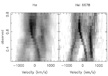
Figure 1.  : The observed line flux from IP Peg as a function of the binary phase with H_α on the left and HeI(6678) on the right; these figures are taken from Steeghs et al.(1997)

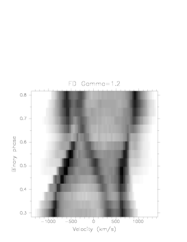
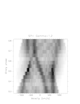
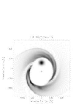
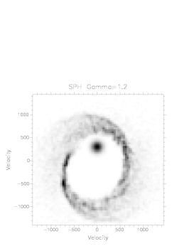
Figure 2.  : Top row: calculated line flux as a function of the binary phase (vertical axis). The horizontal axis represents the radial velocity. Middle row: calculated Doppler map. The horizontal axis and the vertical axis depict the horizontal velocity, $v_{x}$, and the vertical velocity, $v_{y}$, respectively. The bottom row shows the density distribution. The left column shows the results based on the SFS method, while the right column shows those based on the SPH method

References

- [] Godon P., Livio M., Lubow S., 1998, MNRAS, 295, L11.
- [] Jyounouchi T., Kitagawa I., Sakashita, Yasuhara M., 1993, Proceedings of 7th CFD Symposium.
- [] Sawada K., Matsuda T., Hachisu I., 1986a, MNRAS, 219, 75.
- [] Sawada K., Matsuda T., Hachisu I., 1986b, MNRAS, 221, 679.
- [] Sawada K., Matsuda T., Inoue M., Hachisu I., 1987, MNRAS, 224, 307.
- [] Shakura N.I., Sunyaev R.A., 1973, A&A, 24, 337.
- [] Shima E., Jyounouchi T., 1994, 25th Annual Meeting of Space and Aeronautical Society of Japan, pp.36-37.
- [] Steeghs D., Harlaftis E.T., Horne K., 1997, MNRAS, 290, L28.
- [] Yukawa H., Boffin H.M.J., Matsuda T., 1997, MNRAS, 292, 321.