On the Nature of Pulsar Radio Emission

Abstract

A theory of pulsar radio emission generation, in which the observed waves are produced directly by maser-type plasma instabilities operating at the anomalous cyclotron-Cherenkov resonance $\,\omega-\,k_{\parallel}v_{\parallel}+\,\omega_{B}/\,\gamma_{res}=0$ and the Cherenkov-drift resonance $\,\omega-\,k_{\parallel}v_{\parallel}-k_{\perp}u_{d}=0$, is capable of explaining the main observational characteristics of pulsar radio emission. The instabilities are due to the interaction of the fast particles from the primary beam and the tail of the distribution with the normal modes of a strongly magnetized one-dimensional electron-positron plasma. The waves emitted at these resonances are vacuum-like, electromagnetic waves that may leave the magnetosphere directly. In this model, the cyclotron-Cherenkov instability is responsible for core emission pattern and the Cherenkov-drift instability produces conal emission. The conditions for the development of the cyclotron-Cherenkov instability are satisfied for both typical and millisecond pulsars provided that the streaming energy of the bulk plasma is not very high $\,\gamma_{p}\approx 10$. In a typical pulsar the cyclotron-Cherenkov and Cherenkov-drift resonances occur in the outer parts of magnetosphere at $r_{res}\,\approx 10^{9}{\rm cm}$. This theory can account for various aspects of pulsar phenomenology including the morphology of the pulses, their polarization properties and their spectral behavior. We propose several observational tests for the theory. The most prominent prediction are the high altitudes of the emission region and the linear polarization of conal emission in the plane orthogonal to the local osculating plane of the magnetic field.

1 Introduction

More than twenty five years have passed since the discovery of pulsars and there is still no consensus on the basic emission mechanism. At the present time, there are about a dozen competing theories which differ both in the physical effects responsible for the radiation and in the locations where they operate (Melrose (1995)). Probably the only point of agreement between all these theories is the association of pulsars with magnetized, rotating neutron stars. By contrast, there is so much observational data available that none of the existing theories can explain all the main observational facts.

There are several reasons that have precluded understanding of pulsar radio emission. First, there is the unusual physical conditions found in pulsar magnetospheres (relativistic electron-positron plasma, superstrong magnetic fields, ultrarelativistic beam). Secondly, only a small fraction of the energy lost by a neutron star is re-emitted in the radio (even in the high energy range, where a considerable portion of energy is emitted, there is still no consensus on the origin of this emission, e.g., Daugherty & Harding (1996), Romani (1996)). The third reason is that after thirty years of research, we still do not know the general structure of a pulsar magnetosphere (Mestel (1995)). We understand only particular features, like the existence of open and closed field lines and where electric field can be parallel to the magnetic field.

To date, the most widely discussed theory attributes the emission to coherent curvature emission by bunches of particles. Though this theory can explain a broad range of observed pulsar properties by the careful arrangement of the magnetic field geometry and of the form and size of bunches, thirty years of theoretical efforts have failed to explain the origin of these bunches (Melrose (1995)). This theory can also be ruled out on the observational grounds (Lesch et al. (1998)). In addition to the work of Lesch et al. (1998) we note, that this theory also fails to explain the observed correlations of the conal peaks Kazbegi et al. 1991a and a large size of the emitting region Gwinn et al. (1997) (see Section 2).

We propose that the pulsar radiation is generated by plasma instabilities developing in the outflowing plasma on the open field lines of the pulsar magnetosphere. Plasma can be considered as an active medium that can amplify its normal modes. In the case of the two instabilities discussed below, the wave amplification is due to the resonant wave-particle interaction, i.e., in the rest frame of the particle the frequency of the resonant wave is zero or a multiple of the gyrational frequency. The plasma instabilities that we argue operate in the pulsar magnetosphere may be described by the (somewhat contradictory) term ”incoherent broadband maser”. Each single emission by a charged particle is due to the stimulated, as opposed to spontaneous, emission process (hereby the term maser). Unlike the conventional lasers in which basically one single frequency gets amplified, in this case charged particles can resonate with many mutually incoherent waves with different frequencies.

In this paper we discuss a theory of pulsar radio emission developed by Lominadze, Machabeli & Mikhailovskii (1979), Machabeli & Usov (1989), Kazbegi et al. 1991b , Kazbegi et al. 1991c , Lyutikov 1998b , Lyutikov, Machabeli & Blandford (1998). We hypothesize, that pulsar radiation is generated by the instabilities developing in the outflowing plasma on the open field lines in the outer regions of the pulsar magnetosphere. Radiation is generated by two kinds of electromagnetic plasma instabilities – cyclotron-Cherenkov and Cherenkov-drift instabilities. The cyclotron-Cherenkov instability is responsible for the generation of the core-type emission and the Cherenkov-drift instability is responsible for the generation of the cone-type emission (Rankin (1990)). The waves generated by these instabilities are vacuum-like electromagnetic waves so that they may leave magnetosphere the directly.

In contrast to most modern theories of pulsar radio emission, cyclotron-Cherenkov and Cherenkov-drift instabilities occur in the outer parts of magnetosphere. The location of the emission region is determined by the corresponding resonant condition for the cyclotron-Cherenkov and Cherenkov-drift instabilities. Instabilities develop in a limited region on the open field lines. The size of the emission region is determined by the curvature of the magnetic field lines, which limits the length of the resonant wave-particle interaction. The location of the cyclotron-Cherenkov instability is restricted to those field lines with large radius of curvature, while the Cherenkov-drift instability occurs on field lines with curvature bounded both from above and from below. Thus, both instabilities produce narrow pulses, though they operate at radii where the opening angle of the open field lines is large.

To a large extent a possible mechanism for the generation of pulsar radio emission is predicated on the choice of parameters of the plasma flow that is generated by a rotating neutron star. At this point we know only the general features of the distribution function of the particles in a pulsar magnetosphere (Tademaru (1973),Arons 1981b , Daugherty & Harding (1983)). It is believed to comprise (see Fig. 1) (i) a highly relativistic primary beam with the Lorentz factor $\,\gamma_{b}\approx 10^{7}$ and density equal to the Goldreich-Julian density $n_{GJ}={\bf\Omega\cdot B}/(2\,\pi\,e\,c)$, (ii) a secondary electron positron plasma with a bulk streaming Lorentz factor $\,\gamma_{p}\approx 10-1000$, a similar scatter in energy $T_{p}\approx\,\gamma_{p}$ and a density much larger than the beam density $n_{p}\approx\,\lambda\,n_{GJ}=10^{3}-10^{6}n_{GJ}$, (iii) a tail of plasma distribution with the energy up to $\,\gamma_{t}=10^{4}-10^{5}$.

The choice of a particular distribution function (Fig. 1) is very important. All the following is dependent on this choice. In particular, in our model, the primary beam is composed of electrons or positrons. We show in Appendix F that both cyclotron-Cherenkov and Cherenkov-drift instabilities do not develop in an ion beam.

The electromagnetic cyclotron-Cherenkov and Cherenkov-drift instabilities are the strongest instabilities in the pulsar magnetosphere (Lyutikov 1997e ). This differs from the more common case of a nonrelativistic plasma, where electrostatic Cherenkov-type instabilities (i.e. those that result in emission of electrostatic Langmuir-type waves) are generally stronger than electromagnetic instabilities. In addition, for a one-dimensional plasma streaming along the magnetic field, the effective parallel mass is considerably increased by relativistic effects. For the particles in the primary beam, which contribute to the development of the instability, the effective parallel mass is $m_{eff\parallel}\,=\,\gamma_{b}^{3}m\approx 10^{21}\,m$ ($m$ is a mass of a particle). This suppresses the development of the electrostatic instabilities. In contrast, the effective transverse mass , $m_{eff\perp}=\gamma_{b}m$, is less affected by the large parallel momentum. The electromagnetic instabilities are less suppressed by the large streaming momenta. Thus, the relativistic velocities and one-dimensionality of the distribution function result in a strong suppression of the electrostatic instabilities and strengthen electromagnetic instabilities.

Cyclotron-Cherenkov generation of wave by fast particles is not new in astrophysics. For example, cosmic rays in the interstellar medium and in supernova shocks generate Alfvén by a similar mechanism. In the case of Alfvén waves in the nonrelativistic electron-ion plasma, the frequency of the waves $\omega$ can be much smaller than the $kv$ term and can be neglected in the resonance condition. The important difference between these applications and cyclotron-Cherenkov instability in pulsar magnetosphere is that the generated waves belong not to the hydromagnetic Alfvén waves, that cannot leave the plasma, but to near vacuum electromagnetic waves.

We should also mention that a cyclotron-Cherenkov instability of an electron beam propagating along a magnetic field is known in the laboratory as a very effective source of the high frequency microwave radio emission (Galuzo et al. (1982), Didenko et al. (1983), Nusinovich et al. (1995)). The so called slow-wave electron cyclotron masers (ECM) provides a high efficiency and high power microwave source. Though there are no commercial slow-wave ECM available now, they are believed to be very promising devices due to their better control of the beam quality and potentially more compact design than the cyclotron autoresonance masers. Thus, pulsars can be regarded as cosmic slow-wave ECMs.

In previous work (Lyutikov, Machabeli & Blandford (1998)) we developed a new approach to the amplification of curvature radiation. We argue, that a new, Cherenkov-drift instability, may be operational in the pulsar magnetosphere. The Cherenkov-drift emission combines the features of both Cherenkov and curvature emission processes. This instability is similar to the drift instabilities of the inhomogeneous plasma. The striking feature is that, unlike the nonrelativistic laboratory plasma, where drift instabilities develop on the low frequency waves with the wave length on the order of the inhomogeneity size, in the strong relativistic plasma drift instabilities can produce high frequency waves. We develop an approach that treat Cherenkov and curvature emission consistently in cylindrical coordinates. The choice of cylindrical coordinates allows one to consider curvature emission as a resonant emission process. (in the former approaches the wave-particles interaction length was very limited, that precluded a strong amplification under all circumstances). Another important difference in this work is the proper account of the dispersion and polarization of the normal modes. We show that Cherenkov-drift instability develops only in a medium which supports subluminous waves.

We argue that the theory based on the cyclotron-Cherenkov and Cherenkov-drift instabilities is capable of explaining a very broad range of the pulsars’ observed properties. In a ”standard” pulsar with a surface magnetic field $B=10^{12}\,G$ and a period $P=0.5$ s both cyclotron-Cherenkov and Cherenkov-drift instabilities occur at a radius of about $10^{9}$ cm. In a dipole geometry the emission region is limited to the field lines near the direction of the magnetic moment of the neutron star. The emission region for the Cherenkov-drift instability is larger than for the cyclotron-Cherenkov instability. In both cases it is determined by the curvature of the magnetic field lines that limit the coherent growth of the waves.

In Section 2 we shortly review the observational properties of the pulsar radio emission. In Section 3 we discuss the microphysics of the underlying cyclotron-Cherenkov and Cherenkov-drift instabilities. In Section 4 we describe the fiducial pulsar model, and finally in Section 5 we show how the properties of the pulsar radio emission may be explained in the framework of this theory.

2 Observational properties and phenomenological theory of pulsar radio emission

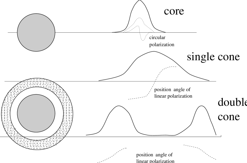
Figure 2: Example of emission geometry that produces core and cone profiles.

A useful observational framework for discussing theory is a description of pulsar radio emission given by Rankin (1990). The main feature of this model is the division of emission into two main classes: core and cone. There may be many cones of emission. In each pulsar the averaged profile may be a combination of core and/or cone emissions (Fig. 2).

The majority of pulsars (about 70$\%$) show core-type emission. The typical core emission has the following features: (a) the profile has a single component, (b) variable circular polarization (up to 60$\%$), the amount of the circular polarization either reaches maximum at the maximum intensity or the sense of polarization may reverse in the middle of the pulse (Fig. emissiongeometry), (c) linear polarization changes from nearly 100$\%$ to unpolarized, in most cases the radiation may be split into two orthogonally polarized modes (Stinebring et al. (1984)).

About 30$\%$ of all pulsars show pure conal emission and they are divided into two main groups – cone singles and cone doubles which are believed to be closely connected, the only difference being the geometrical path of the line of sight through emission region. Conal type emission shows a great variety of phenomena. Some of the typical features of conal emission are (a) the profiles can have up to four components, corresponding to two cones, (b) circular polarization is small and unsystematic, (c) linear polarization is moderate, some pulsars show a sudden change of position angle by $\pm\pi/2$; in most cases the radiation may be split into two orthogonally polarized modes, then the change of position angle by $\pm\pi/2$ corresponds to the change in the relative intensity of the modes. Besides these phenomena, cone-type emission shows drifting subpulses, nullings and mode switching. These effects are probably related to the temporal and/or spatial modulations of the parameters of the outflowing plasma and will not be discused here (see Kazbegi et al. (1996)).

There have been contradictory attempts to determine observationally the emission altitude but this conclusion is model-dependent. By contrast, Gwinn et al. (1997) used interstellar scattering to measure directly the size of the emission region of $\approx 500$ km ($\approx 0.1c/\Omega$). The other, model-dependent, observational evidences for high emission altitudes comes from the large duty cycles often observed in pulsars (”wide beam pulsars”, e.g., Lyne & Manchester (1988)). Conventionally, these pulsars are interpreted as almost aligned rotators. An alternative explanation is that the emission may be coming from large radii.

Another class of pulsars, those with interpulses, are conventionally interpreted as orthogonal rotators with emission coming from two poles despite the fact that emission bridges are often observed in these pulsars Hankins & Fowler (1986) and, at least in one case, PSR B0950+08 the polarization data imply a nearly aligned rotator (Manchester (1995)). The Crab pulsar also has a bridge of emission between the two pulses, intensities of the main pulse and interpulse are correlated and the angle of linear polarization in the two pulses seems to be related. In addition, it shows additional emission peaks between the interpulse and pulse at centimeter wave length Moffett & Hankins (1996). Manchester (1996) suggests that interpulses come from the same pole. If so, the simplest interpretation is that emission originates at high altitudes.

3 Cyclotron-Cherenkov and Cherenkov-drift instabilities

In this section we consider the physics of the cyclotron-Cherenkov and Cherenkov-drift instabilities (Ginzburg & Eidman (1959), Lyutikov, Machabeli & Blandford (1998)). The terminology used here to describe these instabilities refers to the fact that in the cyclotron-Cherenkov emission, a resonant particle changes its gyrational state (undergoes a transition between different Landau level), thereby comes the ”cyclotron” part of its name, but the force that induces the emission is due to the presence of a medium (the ”Cherenkov” part of the name). The Cherenkov-drift emission is similar to conventional Cherenkov (the gyrational state of the resonant particle remains unchanged) but it involves a nonvanishing curvature drift of the resonant particles.

The interplay between cyclotron (or synchrotron) and Cherenkov radiation has been a long-standing matter of interest. Schwinger et al (1976) discussed the relation between these two seemingly different emission mechanisms. They showed that conventional synchrotron emission and Cherenkov radiation may be regarded as respectively limiting cases of $|n-1|\,\ll\,1$ and $B=\,0$ of a synergetic (using the terminology of Schwinger et al. Schwinger et al (1976)) cyclotron-Cherenkov radiation. In the work ( Lyutikov, Machabeli & Blandford (1998) this analogy has been extended to include inhomogeneity of the magnetic field.

The physical origin of the emission in the case of Cherenkov-type and synchrotron-type processes is quite different. In the case of Cherenkov-type process, the emission may be attributed to the electromagnetic polarization shock front that develops in a dielectric medium due to the passage of a charged particle with speed larger than phase speed of waves in a medium. It is virtually a collective emission process. In the case of synchrotron-type process, the emission may be attributed to the Lorentz force acting on a particle in a magnetic field. Cherenkov-type emission is impossible in vacuum and in a medium with the refractive index smaller than unity.

Both the cyclotron-Cherenkov and Cherenkov-drift instabilities, that we believe can develop in pulsar magnetosphere, operate in the kinetic regime, i.e. they are of a maser type (Lyutikov 1998a ). This means that there is some kind of population inversion in the phase space, which supplies the energy for the development of the instability. In the present case, the source of free energy is the anisotropic distribution function of the fast particles. The condition of a population inversion may be restated that the induced emission dominates over induced absorption for a given transition.

The first two steps in identifying the possible maser-type radio emission generation mechanism are (i) determining which radiative transitions are allowed in a given system and (ii) establishing if the given distribution function allows for the population inversion for the particle in resonance with the emitted waves. In this chapter we will first discuss the microphysics of the two suggested emission mechanisms and then show that the distribution function of the particles present on the open field lines of pulsar magnetosphere does have a population inversion and allows maser action. When discussing the microphysics of the emission process, we will concentrate on the spontaneous emission processes. The induced emission rate, which is important for the development of the instabilities, is derivable from the spontaneous emission in the usual manner. In the process of induced emission, the electron emits a wave in phase with the incident wave. However, both cyclotron-Cherenkov and Cherenkov-drift masers are broadband and incoherent because a single electron can resonate with several waves simultaneously.

3.1 Physics of Cyclotron-Cherenkov Emission

The cyclotron-Cherenkov instability develops at the anomalous cyclotron resonance

$$\,\omega({\bf k})-k_{\parallel}v_{\parallel}+{\,\omega_{B}\over\gamma}=0$$ (1)

where $\,\omega({\bf k})$ is the frequency of the normal mode, ${\bf k}$ is a wave vector, $v$ is the velocity of the resonant particle, $\,\omega_{B}=|e|B/mc$ is the nonrelativistic gyrofrequency, $\,\gamma$ is the Lorentz factor in the pulsar frame, $e$ is the charge of the resonant particle, $m$ is its mass and $c$ is the speed of light. Note a sign before the $\,\omega_{B}$ term.

To describe the microphysics of the cyclotron-Cherenkov emission emission process we first recall the microphysics of the conventional Cherenkov emission (Ginzburg & Eidman (1959)). Consider a charged particle propagating in an unmagnetized dielectric with the dielectric constant $\epsilon>1$. As the particle propagates, it induces a polarization in a medium. If the velocity of the particle is larger than the velocity of propagation of the polarization disturbances in a medium, which is equal to the phase speed of the waves $v_{ph}=c/\sqrt{\epsilon}\,<c$, the induced polarization cannot keep up with the particle. This results in a formation of the polarization shock front. At large distances, the electromagnetic fields from this ”shock front” have a wave-like form corresponding to Cherenkov emission. Thus the emission is attributed to the polarization shock front and not directly to the particle. This polarization shock front acts on the particle with a drag force, which slows down the particle. This drag force may be considered as a generalization of the radiation reaction force in a medium.

Now let us consider the propagation of a particle in a magnetized dielectric along a spiral trajectory. Similarly, the propagating charged particle induces polarization in a medium. If the velocity of the particle is larger than the phase speed of the waves, a polarization shock front develops, which acts on the particle with a drag force. Now the drag force, averaged over the gyrational period, has two components: along the external magnetic field and perpendicular to it. The parallel part of the drag force always slows the particle down. The surprising result is that the perpendicular component of the drag force acts to increase the transverse momentum of the particle. Thus a particle undergoes a transition to the state with higher transverse momentum and emits a photon. The energy is supplied by the parallel motion.

The photons emitted by such mechanism correspond to the anomalous Doppler effect $\,\omega-\,k_{\parallel}v_{\parallel}-s\,\omega_{B}/\,\gamma_{res}=0$, with $s\,<0$. In a vacuum, only the normal Doppler resonance, with $s\,>0$, is possible. The necessary condition for the anomalous Doppler effect, $\,\omega-\,k_{\parallel}v_{\parallel}\,<\,0$, may be satisfied for fast particles propagating in a medium with the refractive index larger than unity. It is natural to attribute the emission at the normal Doppler resonances to the Lorentz force of the magnetic field acting on the electron, while the emission at the anomalous Doppler resonances is attributed to the electromagnetic drag forces from the medium.

It may also be instructive to consider the emission process in the frame associated with the center of gyration of the particle. In that frame the waves emitted at the anomalous Doppler effect have negative energy, so that in the emission process the particles increases its energy and emits a photon.

The cyclotron-Cherenkov instability may be considered as a maser using the induced cyclotron-Cherenkov emission. The free energy for the growth of the instability comes from the nonequilibrium anisotropic distribution of fast particles. The condition that the emission rate dominates the absorption requires population inversion in the distribution function of fast particle (maser action). Since radiation reaction due to the anomalous Doppler effect induces transition up in quantum levels , for the instability to occur we need more particles on the lower levels. From the kinetic point of view, waves grow if the quantity ${\bf k}\,{\partial f({\bf p})\over\partial{\bf p}}$ is positive for some values of ${\bf k}$. For an electron in a magnetic field this condition takes the form

$${s\,\omega_{b}\over v_{\perp}}{\partial f\over\partial p_{\perp}}+k_{\parallel}{\partial f\over\partial p_{||}}\,>0$$ (2)

where $s$ is a harmonic number. Here $s>0$ corresponds to normal Doppler effect (transition down in Landau levels) and $s<0$ corresponds to anomalous Doppler effect (transition up in Landau levels). If the distribution function is a plateau-like in parallel momenta then the condition for instability is $s{\partial f\over\partial p_{\perp}}>0$ which could be satisfied for inverted population for the normal Doppler effect or for the ”direct” distribution for anomalous Doppler effect. The latter case takes place for the beam of particles propagating along the magnetic field with no dispersion in transverse momenta.

3.2 Physics of Cherenkov-Drift Emission

There is a possibility for the development of the Cherenkov-drift instability, which occurs at the resonance

$$\,\omega({\bf k})-k_{\parallel}v_{\parallel}-k_{\perp}u_{d}=0$$ (3)

where $u_{d}=\,\gamma v_{\parallel}c/\,\omega_{B}R_{B}$ is the drift velocity, $R_{B}$ is the curvature radius of the magnetic field line. A weak inhomogeneity of the magnetic field results in a curvature drift motion of the particle perpendicular to the local plane of the magnetic field line. A gradient drift (proportional to $({\bf B\cdot\nabla}){\bf B}$ much smaller than the curvature drift and will be neglected. When the motion of the particle parallel to the magnetic field is ultrarelativistic, the drift motion can become weakly relativistic even in a weakly inhomogeneous field resulting in the generation of electromagnetic, vacuumlike waves. The presence of three ingredients (strong but finite magnetic field, inhomogeneity of the field and a medium with the index of refraction larger than unity) is essential for this type of emission. We will call this mechanism Cherenkov-drift emission stressing the fact that microphysically it is virtually Cherenkov-type emission process.

Conventional consideration of the curvature emission (Blandford (1975), Zheleznyakov & Shaposhnikov (1979), Luo & Melrose 1992a , Melrose 1978b ) emphasize the analogy between curvature emission and conventional cyclotron emission. To our opinion this approach, though formally correct, has limited applicability and misses some important physical properties of the emission mechanism. It has two important shortcomings. The first is that in adopting a plane wave formalism, the interaction length for an individual electron, $\approx R_{B}/\gamma_{b}$, is essentially coextensive with the region over which the waves interact with a single electron. The approach necessarily precludes strong amplification under all circumstances because the wave would have to grow substantially during a single interaction in a manner that could not be easily quantified. The second problem was a neglect of dispersion. We address the first shortcoming by expanding the electromagnetic field in cylindrical waves centered on $r=0$, and the second explicitly by considering general plasma modes.

In a separate approach Kazbegi et al. Kazbegi et al. 1991b considered this process calculating a dielectric tensor of an inhomogeneous magnetized medium, thus treating the emission process as a collective effect. They showed that maser action is possible only if a medium supports subluminous waves. In the previous work (Lyutikov, Machabeli & Blandford (1998) we showed how these two approaches can be reconciled and argue that the dielectric tensor approach, which treats the Cherenkov-drift emission as a collective process, has a wider applicability.

It is more natural to consider Cherenkov-drift emission in a curved magnetic field as an analog of the Cherenkov emission with the drift of the resonance particles taken into account, than as the type of a curvature emission. From the microphysical point of view the emission is again due to the polarization shock front that develops due to the passage of a superluminal particle through a medium, so it is required that the emitting particle propagates with the velocity greater than the phase velocity of the emitted waves. The Cherenkov-drift maser is impossible in vacuum, unlike the curvature emission, which is a close analog of the conventional cyclotron emission and is possible in vacuum. The curvature provides only the drift component of the velocity, which is essential for the coupling the resonant particle to the emitted electromagnetic wave.

In a Cherenkov-type emission the resonant particle can interact only with the part of the electric field parallel to the velocity. Thus, if the drift of the resonant particles perpendicular to the plane of the field line is taken into account, it becomes possible to emit a transverse electromagnetic wave with the electric field along the drift velocity, i.e. perpendicular to the plane of the curved field line (see Fig. 4). The growth occurs on the rising part of the parallel distribution function where ${\partial f_{\parallel}\over\partial p_{\parallel}}>0$. This is satisfied for the particles of the primary beam.

4 Model of the Pulsar Radio Emission

4.1 Plasma generation

Rotating, strongly magnetized neutron stars induce strong electric fields that pull the charges from their surfaces. Inside the closed field lines of the neutron star magnetosphere, a steady charge distribution established, compensating the induced electric field. On the open field lines, the neutron star generates a dense flow of relativistic electron-positron pairs penetrated by a highly relativistic electron or positron beam. The density of the primary beam is roughly equal to the Goldreich-Julian density $n_{GJ}={\bf\Omega\cdot B}/(2\,\pi\,e\,c)$. We will normalize the density of the pair plasma to the Goldreich-Julian density.

$$n_{p}=\lambda\,n_{GJ}=10^{3}-10^{6}n_{GJ},\hskip 21.68121pt\omega_{p}^{2}=\lambda\omega_{b}^{2}=2\lambda\omega_{B}\Omega$$ (4)

where $\lambda$ is the multiplicity factor which is the number of pairs produced by each primary particle. Secondary pairs are born with almost the same energy in the avalanche-like process above in the polar cap (Arons (1983)). The pair creation front in the polar cap region is expected to be very thin so we can in the first approximation neglect the residual electric field in the front that could lead to the reversed current and different initial energies and densities of secondary particles. The combination of the pair plasma and primary beam is expected to screen the rotationally induced electric field so that the flow is force-free.

Another relation between the parameters of the plasma and the beam comes from the energy argument that the primary particles stop producing the pairs when the energy in the pair plasma becomes equal to the energy in the primary beam:

$$2\,<\,\gamma\,>^{(0)}_{\pm}\,\lambda\approx\gamma_{b},\hskip 43.36243pt\mbox{at the pair formation front}$$ (5)

where it was assumed that the initial densities, temperatures and velocities of the plasma components are equal. For cold components $<\,\gamma\,>^{(0)}_{\pm}\,=\,\gamma_{p}$ while for the relativistic components with a temperature $T_{p}$ the average energy is $<\,\gamma\,>^{(0)}_{\pm}\,=\,2\,\gamma_{p}\,T_{p}$. The assumption of equipartition (5) is very approximate one, but it allows considerable simplification of numerical estimates. If for some reason, this would turn out to be an incorrect assumption, the corresponding formula can be adjusted by changing the scaling.

As an estimate of the densities of the particles from the tail of plasma distribution we will use the assumption that the energy in the tail is approximately equal to the energy in the plasma (and in the beam):

$$\,\gamma_{t}n_{t}\approx\,\gamma_{b}^{(0)}$$ (6)

where $\,\gamma_{t}$ and $n_{t}$ are the typical energy and the density of the tail particles.

4.2 Typical pulsar

In this work we will make numerical estimates for the ”typical” pulsar with the following parameters:

(i) magnetic field is assumed to be dipole with the magnetic field strength at the surface of neutron star $B_{NS}=\,10^{12}G$,

(ii) rotational period of the star $P=0.5\,$ s (light cylinder radius $R_{LS}=2.4\times 10^{9}$ cm).

(iii) average streaming energy of the plasma components $\gamma_{p}=10$

(iv) temperature of the plasma components $T_{p}=10$.

(v) initial energy of the primary beam at the pair formation front $\gamma_{b}=6\times 10^{7}$.

The energy of the beam will decrease due to the curvature radiation reaction force (Appendix E). Then at the light cylinder, where the instabilities occur, the beam will decelerate due to the curvature radiation reaction to $\,\gamma_{b}=2\times 10^{6}$.

For a given period and magnetic field the equation (5) reduces the number of free parameters for the plasma to two: the plasma temperature and the bulk streaming energy $\,\gamma_{p}$ (or temperature and the multiplicity factor $\,\lambda$). We chose a strongly relativistic plasma with the invariant temperature $T_{p}=10$. The multiplicity factor $\lambda$ corresponding to these parameters follows from Eq. (5): $\lambda=3\times 10^{5}$. The average energy of the tail particles is assumed to be $\,\gamma_{t}=10^{5}$. An important factor that determines the growth rate of the instabilities is the energy scatter of the resonant particles. In estimating the growth rates of the cyclotron-Cherenkov and Cherenkov-drift instabilities on the primary beam we will also assume that the scatter in Lorentz factors of the primary particles in the pulsar frame $\,\Delta\gamma=10^{2}$. This assumes that the beam has cooled considerably due to the curvature radiation and lost about 90% percent of its energy.

Several points are important in our choice of parameters. First, we use a relatively low plasma streaming $\,\gamma$-factor (and respectively high multiplicity factor $\,\lambda$). In the polar cap models (Arons 1981a , Arons (1983)) the pulsar plasma will have a low streaming $\,\gamma$-factor if the the magnetic field near the surface differs considerably from the dipole field thus reducing the radius of curvature (Machabeli & Usov (1989)). Secondly, the required scatter in energy of the primary beam particles ($\Delta\gamma=10^{2}$) is very small. This is due to the effects of curvature radiation reaction on the primary beam during its propagation through the dipole pulsar magnetosphere. The highly nonlinear damping rate due the emission of curvature radiation by the primary beam result in an effective cooling of the beam (see Appendix E).

We used two types of the particle distribution function to calculate the relevant moments: water bag and relativistic Maxwellian (Lyutikov 1998a ). For the case of relativistic Maxwellian distribution function the strongly relativistic temperature $T_{p}=10$ implies that, formally, there are many backward streaming particles. We note, though, that the backward streaming particles do not contribute significantly to any of the relevant moments of the distribution function, so that we can regard the strongly relativistic streaming Maxwellian distribution as a fair approximation to the relatively unknown, but definitely very hot, real distribution function.

The location of our typical pulsar on the $P-\dot{E}$ diagram is shown on Fig 3. The corresponding plasma densities and frequencies are given in Tables 1 and 2 for the two locations (near the stellar surface and at the emission region $R\approx 10^{9}$ cm in the pulsar and plasma reference frames.

	Pulsar frame	Plasma frame
Magnetic field, G	$10^{12}$	$10^{12}$
Cyclotron frequency ${\omega_{B}}^{\ast}$, $({\rm rad\,s^{-1}})$,	$1.8\times 10^{19}$	$1.8\times 10^{19}$
Beam density, $cm^{-3}$	$n_{GJ}^{\prime}\,=\,\Omega B/(2\,\pi\,e\,c)=1.4\times 10^{11}$	$n_{GJ}\,=\,\Omega B/(2\,\pi\,e\,c\gamma_{p})=1.4\times 10^{10}$
Beam plasma frequency, ${\rm rad\,s^{-1}}$	$\omega_{GJ}^{\prime}\,=\,\sqrt{{4\,\pi\,q^{2}\,n_{GJ}^{2}\over m}}\,=\,\sqrt{2\Omega\omega_{B}}\,=\,2\times 10^{10}$	$\omega_{GJ}\,=\,{\omega_{GJ}^{\prime}\over\sqrt{\gamma_{p}}}\,=\,\sqrt{{2\Omega\omega_{B}\over\gamma_{p}}}\,=\,6.3\times 10^{9}$
Beam energy	$\gamma_{b}^{\prime}\,=\,6\times 10^{7}$	$\gamma_{b}\,=\,{\gamma_{b}^{\prime}\over 2\gamma_{p}}\,=\,3\times 10^{6}$
Plasma density, $cm^{-3}$	$n_{p}^{\prime}\,=\,{\lambda\,\Omega\,B\over 2\,\pi\,e\,c}=4\times 10^{16}$	$n_{p},=\,{\lambda\,\Omega B\over 2\,\pi\,e\,c\gamma_{p}}=4\times 10^{15}$
Plasma frequency, ${\rm rad\,s^{-1}}$	$\omega_{p}^{\prime}\,=\,\sqrt{2\,{\omega_{B}}\,\Omega\,\lambda}=1.2\times 10^{13}$	$\omega_{p}\,=\,\sqrt{{2\,{\omega_{B}}\,\Omega\,\lambda\over\gamma_{p}}}\,=\,4\times 10^{12}$
$1-\beta_{X}$, $\beta_{X}$- phase speed of X mode	$\phantom{{{{{a\over b}\over{a\over b}}}\over{{{a\over b}\over{a\over b}}}}}\delta^{\prime}={\omega_{p}^{\prime\,2}T_{p}\over 4\gamma_{p}^{3}\omega_{B}^{2}}={\lambda\Omega T_{p}\over 2\gamma_{p}^{3}\omega_{B}}=10^{-15}$	$\delta={\omega_{p}^{2}T_{p}\over\gamma_{p}\omega_{B}^{2}}={2\lambda\Omega T_{p}\over\gamma_{p}\omega_{B}}=4\times 10^{-13}$

Table 1: Plasma parameters at the surface of the neutron star

	Pulsar frame	Plasma frame
Magnetic field, G	$10^{3}$	$10^{3}$
Cyclotron frequency ${\omega_{B}}^{\ast}$, $({\rm rad\,s^{-1}})$,	$1.8\times 10^{10}$	$1.8\times 10^{10}$
Beam density, $cm^{-3}$	$n_{GJ}^{\prime}\,=\,\Omega B/(2\,\pi\,e\,c)=1.4\times 10^{2}$	$n_{GJ}\,=\,\Omega B/(2\,\pi\,e\,c\gamma_{p})=14$
Beam plasma frequency, ${\rm rad\,s^{-1}}$	$\omega_{GJ}^{\prime}\,=\,\sqrt{{4\,\pi\,q^{2}\,n_{GJ}^{2}\over m}}\,=\,6\times 10^{5}$	$\omega_{GJ}\,=\,{\omega_{GJ}^{\prime}\over\sqrt{\gamma_{p}}}\,=\,3\times 10^{5}$
Beam energy	$\gamma_{b}^{\prime}\,\approx\,\times 10^{6}$	$\gamma_{b}\,=\,{\gamma_{b}^{\prime}\over 2\gamma_{p}}\,=\,5\times 10^{4}$
Plasma density, $cm^{-3}$	$n_{p}^{\prime}\,=\,{\lambda\,\Omega\,B\over 2\,\pi\,e\,c}=4\times 10^{7}$	$n_{p},=\,{\lambda\,\Omega B\over 2\,\pi\,e\,c\gamma_{p}}=4\times 10^{6}$
Plasma frequency, ${\rm rad\,s^{-1}}$	$\omega_{p}^{\prime}\,=\,\sqrt{2\,{\omega_{B}}\,\Omega\,\lambda}=4\times 10^{8}$	$\omega_{p}\,=\,\sqrt{{2\,{\omega_{B}}\,\Omega\,\lambda\over\gamma_{p}}}\,=\,1.2\times 10^{8}$
$1-\beta_{X}$,$\beta_{X}$ phase speed of X mode	$\delta^{\prime}={\omega_{p}^{2}T_{p}\over 4\gamma_{p}^{3}\omega_{B}^{2}}={\lambda\Omega T_{p}\over 2\gamma_{p}^{3}\omega_{B}}=5\times 10^{-7}$	$\delta={\omega_{p}^{2}T_{p}\over\gamma_{p}\omega_{B}^{2}}={2\lambda\Omega T_{p}\over\gamma_{p}\omega_{B}}=1.2\times 10^{-4}$
Typical frequency, ${\rm rad\,s^{-1}}$	$\omega^{\prime}\,=\,5\times 10^{9}$	$\omega={\omega^{\prime}\over 2\gamma_{p}}=2.5\times 10^{8}$

Table 2: Plasma parameters at the emission region $R\approx 10^{9}$ cm

The radial dependence of the parameters is assumed to follow the dipole geometry of the magnetic field:

$${\omega_{B}}(r)\,=\,{\omega_{B}}(R_{NS})\left({R_{NS}\over r}\right)^{3},\mbox{}$$

$$\omega_{p}(r)\,=\,\omega_{p}(R_{NS})\left({R_{NS}\over r}\right)^{3/2}.$$ (7)

This may not be a good approximation in the outer regions of the pulsar magnetosphere, where relativistic retardation, currents flowing in the magnetosphere and the effects of plasma loading considerably change the structure of the magnetic field.

4.3 Fundamental plasma modes

It is important for the development of both instabilities that the plasma supported subluminous waves. Such wave indeed exist in a strongly magnetize electron-positron plasma. If we neglect (as a first order approximation) the relative streaming of the plasma electrons and positrons and the field curvature then there are three fundamental modes: transverse extraordinary wave with the electric field perpendicular to the k-B plane and longitudinal-transverse mode the electric field in the k-B with two branches: ordinary mode and Alfvén mode (Arons & Barnard (1986), Volokitin, Krasnosel’skikh & Machabeli (1985), Lyutikov 1998a ). For small angles of propagation with respect to magnetic field the ordinary mode (upper longitudinal-transverse wave) is quasi-longitudinal for small wave vector ($k\ll\,\omega_{p}/c$, $\,\omega_{p}$ - plasma frequency) and quasi-transverse for large wave vector ($k\gg\,\omega_{p}/c$), while the Alfvén mode is quasi-transverse for small wave vector and quasi-longitudinal for large ones. Fig. 5 illustrates these modes in the case of cold plasma components in the plasma frame and in the low frequency limit $\omega^{\prime}\ll\omega_{B}$ ($\omega^{\prime}$ is the wave frequency in the plasma frame).

The dispersion relations for the extraordinary mode in the pulsar frame in the limit $\,\omega\ll\,\omega_{B}$ is

$$\,\omega=kc(1-\delta),\hskip 7.22743pt\delta={\,\omega_{p}^{2}T_{p}\over 4\,\omega_{B}^{2}\,\gamma_{p}^{3}}$$ (8)

where we used a relationship between the plasma density and the Goldreich-Julian density $n_{p}=\,\lambda n_{GJ}$ and the definition of the Goldreich-Julian density.

For the coupled Alfvén and ordinary modes it is possible to obtain the asymptotic expansion of the dispersion relations in the limits of very small and very large wave vectors. Here we will give the dispersion relations for the quasitransverse parts of the waves

$$\,\omega^{2}\,=\, {c^{2}}\,{k^{2}}\,\left(1-{\,\omega_{p}^{2}\,T_{p}\,\over 2\,\gamma_{p}^{3}\,\omega_{B}^{2}}\,+{\frac{2\,\,\gamma_{p}{{\,\omega_{p}}^{2}}T_{p}\,{{\sin^{2}\theta}}}{{c^{2}}\,{k^{2}}\,}}\right)\mbox{ O-wave} kc\,\gg\sqrt{T_{p}}\,\gamma_{p}\omega_{p} \theta<1/T_{p}$$ if and

$$\mbox{}\,\omega^{2}\,=\, {c^{2}}\,{k^{2}}\,\cos^{2}\theta\,\left(1-{\,\omega_{p}^{2}\,T_{p}\,\over 2\,\gamma_{p}^{3}\,\omega_{B}^{2}}\,-{\frac{{c^{2}}\,{k^{2}}\,{{\sin^{2}\theta}}}{2\,T_{p}\,\,\gamma_{p}{{\,\omega_{p}}^{2}}}}\right)\mbox{ Alfv\'{e}n wave} kc\,\ll\,\sqrt{T_{p}}\,\gamma_{p}\omega_{p}$$ if (9)

These relationships are valid for the frequencies satisfying the inequality

$$\,\omega\ll\,\gamma_{p}\,\omega_{B}/T_{p}$$ (10)

This is a condition that in the reference frame of the plasma the frequency of the waves is much smaller that the typical cyclotron frequency of the particles $\,\omega_{B}/T_{p}$.

When the relative streaming of the plasma is taken into account, the dispersion relations change considerably: a new, slow Alfvén branch appears and the extraordinary and Alfvén modes behave differently in the region of small wave vectors (Lyutikov 1998b ). The polarization of the fundamental modes also changes. For the angles of propagation with respect to magnetic field less than some critical angle, which depends on the difference of the velocities of the components and on the magnetic field, the two quasi–transverse waves are circular-polarized, while for the larger angles the two transverse modes become linearly-polarized.

4.4 Development of instabilities

In this section it is shown, that the pulsar radiation may be generated by two kinds of electromagnetic plasma instabilities – cyclotron-Cherenkov and Cherenkov-drift instabilities. The cyclotron-Cherenkov instability is responsible for the generation of the core-type emission and the Cherenkov-drift instability is responsible for the generation of the cone-type emission (Rankin (1990)). The waves generated by these instabilities are vacuum-like electromagnetic waves: they may leave the magnetosphere directly.

We assume that the distribution function, displayed in Fig. 1, remains unchanged throughout the inner magnetosphere. This requires that no Cherenkov-type two-stream instabilities develop and that the high energy particles are not excited to the high gyrational states by the mutual collisions or by the inverse Compton effect. Then the outer regions of the pulsar magnetosphere two instabilities can develop: (i) cyclotron-Cherenkov instability and (ii) Cherenkov-drift instability.

A detailed consideration of the conditions necessary for the development of the cyclotron-Cherenkov and Cherenkov-drift instabilities are given in Appendix A and C. Both cyclotron-Cherenkov and Cherenkov-drift instabilities develop in the outer regions of the pulsar magnetosphere at radii $R\approx 10^{9}$ cm.

The frequencies of the waves generated by the cyclotron-Cherenkov instability are given by (A3)

$$\omega={4\,\gamma_{p}^{3}\omega_{B}^{3}\over\,\gamma_{res}T_{p}\omega_{p}^{2}}$$ (11)

which may be solved for the radius at which the waves with frequency $\omega$ are emitted:

$$R=R_{NS}\left({2\gamma_{p}^{3}\over\lambda\gamma_{res}T_{p}}\right)^{1/6}\,\left({\omega_{B}^{\ast\,2}\over\omega\Omega}\right)^{1/6}=1.8\times 10^{9}\,B_{12}^{1/3}\,\nu_{9}^{-1/6}\,P_{0.5}^{1/6}\gamma_{res,5}^{-1/6}{\rm cm}$$ (12)

The relationship (12) may be regarded as a ”radius-to-frequency” mapping. For a given $\,\gamma_{res}$ the radial dependence of the right hand side of equation (11) will result in a radial dependence of the emitted frequency. The radial dependence of the parameters in (A3) will result in emission of higher frequencies deeper in the pulsar magnetosphere, exactly what is observed. The frequencies emitted at the Cherenkov-drift resonance do not have a simple dependence on radius from the neutron star. They are determined by several emission conditions which limit the development of the instabilities to the particular location in the magnetosphere and particular frequencies.

The conditions that the instabilities should satisfy are:

(i) small growth length in a curved field lines ${c/\Gamma}<\Delta\theta R_{B}$, where $\Delta\theta$ is the range of the emitted resonant angles

(ii) condition of kinetic instability $\left|{\bf k}\delta{\bf v}_{res}\right|\gg\Gamma$

In addition to these, the Cherenkov-drift instability should also satisfy another condition:

(iii) the condition of a large drift $u_{d}/c>\sqrt{2\delta}$.

The condition (i) states that an emitting particle can stay in a resonances with the wave for many growth lengths. The condition (ii) is a requirement that the growth rate of instability is much smaller than the bandwidth of the growing waves. This condition is necessary for the random phase approximation to the wave-particle interaction to apply.

In Appendices A, C and D we show that the above conditions can be satisfied for the chosen set of parameters both in normal pulsar and millisecond pulsars. The conditions for the development of the cyclotron-Cherenkov and Cherenkov-drift instabilities depend in a different ways on the parameters of the plasma. They may develop in the different regions of the pulsar magnetosphere.

5 Pulsar Phenomenology

5.1 Energetics

In both cyclotron-Cherenkov and Cherenkov-drift mechanism, the emission is generated by the fast particles which supply the energy for the growth of the waves. The total energy available for the conversion into radio emission is of the order of the energy of the particle flow along the open field lines of pulsar magnetosphere:

$$E\approx n_{GJ}\,\pi R_{pc}^{2}\,\gamma_{b}mc^{3}\approx 10^{33}{\rm erg\,s^{-1}}$$ (13)

where $R_{pc}=R_{NS}\sqrt{{R_{NS}\Omega\over c}}$ is the radius of a polar cap. This is sufficient to explain the radio luminosities of the typical pulsar if the effective emitting area is about one hundredth of the total open field line cross section.

5.2 Emission Pattern

The emission pattern for the ”core”-type pulsars (according to the classification of (Rankin (1990)) is a circle with the angular extent of several degrees. In our model the region of the cyclotron-Cherenkov instability is limited to the nearly straight field lines (see Fig. 8).

The curvature of the magnetic field destroys the coherence between the waves and the resonant particles. To produce an observable emission the waves need to travel in resonance with the particle at least several instability growth lengths. Far from the magnetic axis, where the curvature is substantial, the waves leave the resonance cone before they travel a growth length and no substantial amplification occurs. Near the magnetic field axis the radius of curvature is very large and waves can stay in a resonance with a particles for a long time and grow to large amplitudes.

By contrast, the Cherenkov-drift instability requires curvature of the field lines, but its growth rate may be limited by the coherence condition. In a dipole geometry, this will limit the Cherenkov-drift emission region to a ring around the central field line. Another possible location of the Cherenkov-drift instability is the region of the swept back field lines (Fig. 8)

The development of the cyclotron-Cherenkov instability depends on fewer parameters than the Cherenkov-drift instability. It develops on the nearly straight central field lines. The conditions for the development of the cyclotron-Cherenkov instability (Eqs. A4, A9, A13) depend on low powers of the plasma parameters, so it is quite robust. By contrast, the Cherenkov-drift instability depends on the plasma parameters and the radius of curvature of the magnetic field in a complicated way. This results in a broader range of phenomena observed in the cone emission. If the parameters of the plasma change due the changing conditions at the pair production front, the location of the Cherenkov-drift instability may change considerably. This may account for the mode switching observed in the cone emission of some pulsars.

It may also possible beto explain in the framework of our model the phenomenon of ”wide beam geometry” observed in some pulsars (Manchester (1996)). The Cherenkov-drift instability may occur in the region, where the field lines are swept back considerably. Then the emission will be generated in what could be called a ”wide beam geometry”.

5.3 Polarization

If the average energy of the electrons and positrons of the secondary plasma is the same, the fundamental modes of such strongly magnetized plasma are linearly polarized. Both of the two quasi–transverse modes (one with electric field lying in the ${\bf k-B_{o}}$ plane, another with ${\bf E}$ perpendicular to this plan) may be emitted by the cyclotron-Cherenkov mechanism. This may naturally explain the two orthogonal modes observed in pulsars (Kazbegi et al. 1991b , Kazbegi et al. 1991c , Lominadze, Machabeli & Usov (1983)). The difference in the dispersion relations and in the emission and absorption conditions between ordinary and extraordinary modes may explain the difference in the observed intensities of these modes.

The rotation of the magnetized neutron star produces a difference in the average streaming velocities of the plasma components. This results in the circular polarization of the quasi–transverse modes for the angles of propagation with respect to the local magnetic field less than some critical angle. This may explain in a natural way the occurrence of the circular polarization in the ”core” emission.

If the cyclotron-Cherenkov instability occurs on the tail of the plasma distribution function then the particles of both signs of charge can resonate with the wave. In a curved magnetic field, electrons and positrons will drift in opposite directions (Fig. 9). As the line of sight crosses the emission region, the observer will first see the left circularly polarized wave emitted by the electrons in the direction of their drift. When the line of sight becomes parallel to the local magnetic field the wave will resonate with both electrons and positrons in the plasma tail, so that the resulting circular polarization will be zero. Finally, the observer will see the wave emitted by positrons in the direction of their drift. This can explain the switch of the circular polarization observed in some pulsars.

The cone emission, which is due to the Cherenkov-drift instability naturally has one linear polarization. An important difference from the standard bunching theory is that the waves emitted at the Cherenkov-drift resonance are polarized perpendicular to the plane of the curved magnetic field line. This may be used as a test to distinguish between the two theories. To do so, one need to determine the absolute position of the rotation axis of a pulsar - a possible but a difficult task. One possible experiment would involve Harrison-Tademaru effect (Harrison & Tademaru (1975)), which predicts that the spins of neutron stars may be aligned with their proper motion due to the quadrupole magnetic radiation if the magnetic moment is displaced from the center of the star. Unfortunately, the current data does not support this theory (in the Crab, the spin of the neutron star is within $10^{o}$ of from the direction of the proper motion, while for Vela it is approximately perpendicular). Symmetry of plerions and direct observation of jets from pulsars (like the one observed in Vela pulsar (Markwardt & Ogelman (1995))) combined with polarimetry of the pulsar may be useful in determining the relative position of the electric field of the wave and the magnetic axis.

5.4 Radius-to-frequency mapping

The cyclotron-Cherenkov mechanism predicts a simple dependence of the emitted frequencies on the altitude (Eq. 12). The predicted power-law scaling of the emission altitudes is $R(\nu)\propto\nu^{-1/6}$. This is strikingly close to the observed scaling $\propto\nu^{-.15\pm.1}$ (Lesch et al. (1998), Kramer et al. (1994)), which is derived from the simultaneous multifrequency observations of the time of arrival of pulses. A simple ”radius-to-frequency” mapping will be ”blurred” by the scatter in energies of the resonant particles, but the general trend that lower frequencies are emitted higher in the magnetosphere will remain.

The Cherenkov-drift instability, on the other hand, does not have a simple dependence of the emission altitudes on the frequency. The resonance conditions for the Cherenkov-drift instability are virtually independent of frequency (Eq. C1), so that the location of the emission region is determined by the various conditions on the development of the instability (Appendix C).

5.5 Formation of Spectra

Development of the Cyclotron-Cherenkov and Cherenkov-drift instabilities results in an exponential growth of the electromagnetic waves. The original growth may be limited by several factors. A very likely possibility is that a spatial growth of the waves is limited by the changing parameters of the plasma. This possibility is hard to quantify since we do not know structure of the magnetic field in the outer regions of the pulsar magnetosphere. The original growth of the instabilities may also be limited by the nonlinear processes: quasi-linear diffusion, induced scattering and wave decay. Finally, as the waves propagate in a magnetosphere, they may be absorbed by the particles of the bulk plasma (Lyutikov 1998a ). The emergent spectra are the combined results of the these processes: emission, nonlinear saturation and absorption.

We have considered the two most likely nonlinear saturation effects for the cyclotron-Cherenkov instability: quasilinear diffusion and induced Raman scattering (Lyutikov 1998c , Lyutikov 1998d ). In the case of quasilinear diffusion, the induced transitions to upper Landau levels due the development of the cyclotron-Cherenkov instability is balanced by the radiation reaction force due to the cyclotron emission at the normal Doppler resonance and the force arising in the inhomogeneous magnetic field due to the conservation of the adiabatic invariant. These forces result in a quasilinear state and a saturation of the quasilinear diffusion. We have found a state, in which the particles are constantly slowing down their parallel motion, mainly due to the component along magnetic field of the radiation reaction force of emission at the anomalous Doppler resonance. At the same time they keep the pitch angle almost constant due to the balance of the force arising in the inhomogeneous magnetic field due to the conservation of the adiabatic invariant and the component perpendicular to the magnetic field of the radiation reaction force of emission at the anomalous Doppler resonance. We calculated the distribution function and the wave intensities for such quasilinear state (Lyutikov 1998d ).

In the process of the quasilinear diffusion, the initial beam looses a large fraction of its initial energy $\approx 10\%$, which is enough to explain the typical luminosities of pulsars. The theory predicts a spectral index $F(\nu)\propto\nu^{-2}$ ($F(\nu)$ is the spectral flux density) which is very close to the observed mean spectral index of $-1.6$ (Lorimer at al. (1995)). The predicted spectra also show a turn off at the low frequencies $\nu\leq 300MHz$ and a flattering of the spectrum at large frequencies $\nu\geq 1GHz$ (this may be related to the upturn in pulsar spectra observed at mm-wavelength, (Kramer et al. (1996))).

The other possible mechanism that may be important for wave propagation and as an effective saturation mechanism for instabilities of electromagnetic waves is induced Raman scattering of electromagnetic waves (Lyutikov 1998c ). The frequencies, at which strong Raman scattering occur in the outer parts of magnetosphere, fall into the observed radio band. The typical threshold intensities for the strong Raman scattering are of the order of the observed intensities, implying that pulsar magnetosphere may be optically thick to Raman scattering of electromagnetic waves.

Absorption processes can play an important role in the formation of the emergent spectra (Lyutikov 1998a ). The waves may be strongly damped on the three possible resonances: Cherenkov, Cherenkov-drift and cyclotron. Alfvén wave is always strongly damped on the Cherenkov resonances and possibly on the Cherenkov-drift resonance and cannot leave magnetosphere. Both ordinary and extraordinary waves may be damped on the Cherenkov-drift resonance. In this case Cherenkov-drift resonance affects only the ordinary and extraordinary waves with the electric field perpendicular to the plane of the curved magnetic field line. The high frequency parts of the extraordinary and ordinary wave may also be damped on the cyclotron resonances. In fact, in a dipole geometry, electromagnetic waves propagating outward are always absorbed. The fact that we do see radiation implies that waves get ”detached” from plasma escaping absorption.

5.6 High Energy Emission

It may be possible also to relate the pulsed high energy emission to the radio mechanisms. The development of the cyclotron-Cherenkov instability at the anomalous Doppler effect leads to the finite pitch angles of the resonant particles. The particles will undergo a cyclotron transition at the normal Doppler effect decreasing the their pitch angle. The frequency of the wave emitted in such a transition will fall in the soft $X$-ray range with the frequencies

$$\omega\approx\gamma_{b}\omega_{B}=\,10^{18}{\rm rad\,s^{-1}}\hskip 14.45377pt(E\approx 1{\rm keV})$$ (14)

In such a model the high energy emission will coincide with the core component of the radio emission, which is what is observed in Crab pulsar and some other pulsars. We also note, that this may be a feasible theory for the pulsed soft $X$-ray emission. The hard $X$-ray and $\,\gamma$-emission cannot be explained by this mechanism since the total energy flux in the primary beam is not enough to account for the very high energy emission (see, for example, Usov (1996)).

6 Observational Predictions

General Predictions of the Maser-type Instability

The formalism of the maser-type emission assumes a random phase approximation for the wave-particle interaction. Any given particle can simultaneously resonate with several waves whose phases are not correlated. This is different from the reactive-type emission (like coherent emission by bunches) when the intensities of the waves with different frequencies are strongly correlated. Thus any observation of the fine frequency structure in the pulsar radio emission may be considered as a strong argument against the reactive-type emission and in favor of the maser-type emission.

Frequency Dependence of the Circular Polarization in the Core

The cyclotron-Cherenkov instability can develop both on the primary beam particles and the particles from the tail of the plasma distribution. The cyclotron-Cherenkov instability on the primary beam produces a pulse which has a maximum circular polarization in its center. The cyclotron-Cherenkov instability on the tail particles produces a pulse with the switching of the sense of the circular polarization in its center. Since the resonance on the tail particles occurs on larger frequencies ( Eq. A3) the effects of the switching sense of the circular polarization should be more prominent on the higher frequencies.

Linear Polarization of the Cone Radiation

Cherenkov-drift instability produces waves with the linear polarization perpendicular to the plane of the curved field line. This is in a sharp contrast to many other theories of the radio emission that tend to generate waves with the electric field in the plane of the curved field line. If one can determine the absolute position of the rotational axis, magnetic moment and the electric vector of the linear polarization, then, assuming a dipole geometry, it will be possible to determine unambiguously the position of the electric vector of the emitted wave with respect to the plane of the magnetic field line.

No Cyclotron-Cherenkov Instability in Millisecond Pulsars

In Appendix D we show that the cyclotron-Cherenkov instability does not develop in the magnetospheres of the millisecond pulsars. Since in our model the cyclotron-Cherenkov instability produces core-type emission we predict that millisecond pulsars will not show core-type emission. At present, the existing observations do not allow a separation into the core and cone type emission in the millisecond pulsars.

7 Conclusion

In this work we presented a model for the pulsar emission generation capable of explaining a broad range of the observations including the morphology, polarization and spectrum formation in normal and millisecond pulsars. We provided no explanation for the temporal behavior, nulling, drifting subpulses although these phenomena do not challenge the model. Our model makes several testable predictions, like high altitude of the emission region and an unusual relation of the polarization direction to the magnetic axis for the cone emission. In addition it has flexibility to accommodate a variety of phenomena arising, for example, due to the temporal variations in the flow and the structure of the magnetic field in a given pulsar, or due to the different structure of the magnetosphere in different pulsars.

Further progress requires a better understanding of the structure of the pulsar magnetospheres both near the stellar surface where the mutipole moments of the magnetic field can substantially affect the physics of the pair formation front, and near the light cylinder, where the emission is taking place. It is also necessary to consider the nonlinear stages of the emission mechanisms described above.

Appendix A Conditions on cyclotron-Cherenkov instability

In this Appendix we consider the development of the cyclotron-Cherenkov instability in magnetosphere of the typical pulsar. We show that the conditions on page 4.4 (Section 4.4) for the development of the cyclotron-Cherenkov instability instability are satisfied for the typical pulsar.

The conditions for the development of the cyclotron-Cherenkov instability may be easily derived for the small angles of propagation with respect to the magnetic field. Representing the wave’s dispersion as

$$\,\omega=kc(1-\delta),\hskip 21.68121pt\mbox{ where }\delta\,=\,\left\{\begin{array}[]{ll}{\,\omega_{p}^{2}T_{p}\over 4\,\gamma_{p}^{3}\,\omega_{B}^{2}}&\mbox{ X mode}\\ {\,\omega_{p}^{2}T_{p}\over 4\,\gamma_{p}^{3}\,\omega_{B}^{2}}-{\,\gamma_{p}\,\omega_{p}^{2}T_{p}\sin^{2}\theta\over k^{2}c^{2}}&\mbox{ O mode}\\ {\,\omega_{p}^{2}T_{p}\over 4\,\gamma_{p}^{3}\,\omega_{B}^{2}}+{k^{2}c^{2}\sin^{2}\theta\over 4\,\gamma_{p}\,\omega_{p}^{2}T_{p}}&\mbox{ Alfv\'{e}n mode}\end{array}\right.$$ (A1)

and neglecting the drift term, the resonance condition (1) may then be written as

$${1\over 2\,\gamma_{res}^{2}}-\delta+{\theta^{2}\over 2}=\,-\,{\,\omega_{B}\over\omega\,\gamma_{res}}$$ (A2)

Let us discuss the condition for the development of the cyclotron-Cherenkov instability. First we note that equation (A2) requires that ${1\over 2\,\gamma_{res}^{2}}\,<\,\delta$ and ${\theta^{2}\over 2}\,<\,\delta$. The first is the condition that the particle is moving through plasma with the velocity faster than the phase velocity of the wave. The second condition limits the emission to the small angles with respect to magnetic field. Assuming that ${1\over 2\,\gamma_{res}^{2}}\,\ll\,\delta$ and ${\theta^{2}\over 2}\,\ll\,\delta$ we find from (A2)

$$\,\omega={\,\omega_{B}\over\gamma_{res}\delta}$$ (A3)

This resonant frequency increases with radius as $R^{6}$.

Using the upper limit on the frequencies for the relations (A1) to hold, namely $\,\omega\ll\,\gamma_{p}\,\omega_{B}/T_{p}$. This sets the limit on $\delta$: $\delta\gg T_{p}/(\,\gamma_{p}\,\gamma_{res})$. This condition is satisfied for the radii:

$$\left({R\over R_{NS}}\right)\,>\,\left({2\,\gamma_{p}^{2}\,\omega_{B,NS}\over\gamma_{b}\,\lambda\Omega}\right)^{1/3}=\left\{\begin{array}[]{ll}\,5\times 10^{2}&\mbox{ for the beam}\\ \,2\times 10^{3}&\mbox{ for the tail}\end{array}\right.$$ (A4)

This is the radius where the resonance condition first becomes satisfied for the particles of the primary beam and from the tail of the distribution function.

The cyclotron-Cherenkov instability growth rate is (e.g., Kazbegi et al. 1991c ):

$$\Gamma=\sqrt{{\pi\over 2}}{\,\omega_{p,res}^{2}\over\omega\,\Delta\gamma}=\sqrt{{\pi\over 2}}{\,\lambda\,\lambda_{res}T_{p}\,\gamma_{res}\over\,\Delta\gamma\,\gamma_{p}^{3}}\,{\Omega^{2}\over\omega_{B}}$$ (A5)

where we have normalized the density of the resonant particles to the Goldreich-Julian density $\,\omega_{p,res}^{2}=\,\lambda_{res}\,\omega^{2}_{GJ}$.

It follows from (A5) that the growth rate increases with radius as $R^{3}$. Deeper in the magnetosphere the growth rate is slow and the waves are not excited. At some point the growth rate becomes comparable to the dynamic time $\Gamma/\Omega=1$. This occurs at

$$\left({R\over R_{NS}}\right)=\left({\,\Delta\gamma\,\gamma_{p}^{3}\over\sqrt{{\pi\over 2}}\,\lambda\,\lambda_{res}T_{p}\,\gamma_{res}}\,{\,\omega_{B}^{\ast}\over\Omega}\right)^{1/3}=\left\{\begin{array}[]{ll}\,2\times 10^{3}&\mbox{ for the beam}\\ \,1\times 10^{3}&\mbox{ for the tail}\end{array}\right.$$ (A6)

Using the equipartition condition (6) we conclude that at a given radius the growth on the tail particles is approximately the same (the higher resonant density is compensated by the higher resonant $\,\gamma$-factor.

Starting this radius the waves will start to grow with the growth rate increasing with radius. The highest frequency of the growing mode is determined by the condition (A3) evaluated at the radius (A6):

$$\,\omega_{max}=\left\{\begin{array}[]{ll}1\times 10^{8}{\rm rad\,s^{-1}}&\mbox{ for the resonance on the beam}\\ 4\times 10^{11}{\rm rad\,s^{-1}}&\mbox{ for the resonance on the tail }\end{array}\right.$$ (A7)

These estimates show, that for the chosen plasma parameters the cyclotron-Cherenkov instability always develops on the tail of the distribution function and can also develop on the particles from the primary beam. The higher density of the tail particles favors the development of the instability on the tail particles. The cyclotron-Cherenkov instability on the tail particles occurs deeper in the magnetosphere on the higher frequencies than the cyclotron-Cherenkov instability on the primary beam, which can develop further out in the magnetosphere and produce emission at the lower frequencies.

The growth rate of the cyclotron-Cherenkov instability should satisfy two other conditions: the growth length must be much less that the length of the coherent wave-particle interaction and the condition of the kinetic approximation. The coherent wave-particle interaction in limited by the curvature of the magnetic field. A particle can resonate with the waves propagating in a limited range of angles with respect to the magnetic field. As the wave propagates in a curved field the angle that the wave vector makes with the field changes and the wave may leave the range of resonant angles. If the range of the resonant angles is $\Delta\theta$ then the condition of a short growth length is

$${c\over\Gamma}<\Delta\theta R_{B}$$ (A8)

For cyclotron-Cherenkov instability we can estimate $\Delta\theta\approx\sqrt{\delta}$. Then we find a condition on the radius of curvature

$$R_{B}>{1\over\sqrt{2\pi}}{c\,\Delta\gamma\over\lambda_{res}\Omega\,\gamma_{res}\delta^{3/2}}\approx\left\{\begin{array}[]{ll}10^{11}{\rm cm}&\mbox{ for the beam}\\ 5\times 10^{10}{\rm cm}&\mbox{ for the tail}\end{array}\right.$$ (A9)

at the distance $R=2\times 10^{9}{\rm cm}$. The region of the cyclotron-Cherenkov instability is limited to the field lines near the central field line. The transverse size of the emission region may be estimated as $x=R^{2}/R_{B}\approx 10^{8}{\rm cm}$. This gives an opening angle of the emission $\theta^{em}=x/R\approx 2^{\circ}$.

There is another condition that the growth rate (A5) should satisfy, namely the condition of the kinetic approximation. In deriving the growth rate we implicitly assumed that the wave-particle interaction is described by the random phase approximation, which requires that the spread of the resonant particles satisfies the condition

$$\left|{\bf k}\delta{\bf v}_{res}\right|\gg\Gamma$$ (A10)

For the particle streaming in the curved magnetic field without any gyration this condition takes the form

$$\left|k_{\parallel}c{\Delta\,\gamma\over\gamma^{3}}+k_{x}u_{d}{\Delta\,\gamma\over\gamma}+{s\,\omega_{B}\Delta\,\gamma\over\gamma^{2}}\right|\gg\Gamma$$ (A11)

For the cyclotron-Cherenkov instability the last term on the left hand side of (A11) is the dominant:

$${\,\omega_{B}\,\Delta\gamma\over\gamma_{res}^{2}}\gg\Gamma$$ (A12)

Using the growth rate (A5) this condition may be rewritten as

$$\left({R\over R_{NS}}\right)\ll\left(\sqrt{{2\over\pi}}{\,\Delta\gamma^{2}\,\omega_{B}^{\ast^{3}}\,\gamma_{p}^{3}\over\lambda_{res}\Omega^{2}\,\gamma_{res}^{3}\,\lambda T_{p}}\right)^{1/6}=3\times 10^{5}$$ (A13)

Equation (A13) means that the kinetic approximation is well satisfied inside the pulsar magnetosphere.

Thus, the conditions for the development of the cyclotron-Cherenkov instability may be satisfied for the typical pulsar parameters. The waves are generated in the observed frequency range near the central field line. The radius of emission is $\approx 10^{9}{\rm cm}$, the transverse size of the emitting region is $\approx 10^{8}{\rm cm}$ and the ”thickness” of the emitting region is $\leq 10^{9}{\rm cm}$. This may account for the core-type emission pattern.

Appendix B Grow rate for the Cherenkov-drift instability

In this Appendix we calculate the growth rate for the Cherenkov-drift instability in the plane wave approximation. Originally this growth rate has been obtained by Lyutikov, Machabeli & Blandford (1998) using the single particle emissivities. Here we give a derivation using the simplified dielectric tensor (Lyutikov, Machabeli & Blandford (1998)). The relevant components of the antihermitian part of the dielectric tensor are (Kazbegi et al. 1991b ).

$$\epsilon^{\prime\prime}_{xx} =-i{4\pi^{2}q^{2}\over\omega c}\int{dp_{\phi}}u_{d}^{2}{\partial f(p_{\phi})\over\partial p_{\phi}}\delta\left(\omega-k_{\phi}v_{\phi}-k_{x}u_{d}\right),\mbox{}$$

$$\mbox{}\epsilon^{\prime\prime}_{x\phi} =-i{4\pi^{2}q^{2}\over\omega c}\int{dp_{\phi}}u_{d}v_{\phi}{\partial f(p_{\phi})\over\partial p_{\phi}}\delta\left(\omega-k_{\phi}v_{\phi}-k_{x}u_{d}\right)=\epsilon^{\prime\prime}_{\phi x},\mbox{}$$

$$\mbox{}\epsilon^{\prime\prime}_{\phi\phi} =-i{4\pi^{2}q^{2}\over\omega}\int{dp_{\phi}}v_{\phi}{\partial f(p_{\phi})\over\partial p_{\phi}}\delta\left(\omega-k_{\phi}v_{\phi}-k_{x}u_{d}\right).$$ (B1)

The growth rate of the Cherenkov drift instability can be obtained from (Melrose 1978b ):

$$\Gamma=\int d{\bf p}w({\bf k},{\bf p})\,\hbar{\bf k}\cdot{\partial f({\bf p})\over\partial{\bf p}}.$$ (B2)

The growth rate for the lt-mode is

$$\Gamma^{lt}={4\pi^{2}q^{2}\over m}\int dp_{\phi}\left({k_{\phi}k_{x}u_{d}\over ckk_{\perp}}-{v_{\phi}\over c}{k_{\perp}\over k}\right)^{2}{\partial f(p_{\phi})\over\partial p_{\phi}}\delta\left(\omega-k_{\phi}v_{\phi}-k_{x}u_{d}\right),$$ (B3)

and growth rate for the t-mode is

$$\Gamma^{t}={4\pi^{2}q^{2}\over m}\int dp_{\phi}\left({k_{r}u_{d}\over k_{\perp}c}\right)^{2}{\partial f(p_{\phi})\over\partial p_{\phi}}\delta\left(\omega-k_{\phi}v_{\phi}-k_{x}u_{d}\right).$$ (B4)

Where we chose the following polarization vectors

$${\bf e^{lt}}={1\over kk_{\perp}}\left\{k_{\phi}k_{r},-k_{\perp}^{2},k_{x}k_{\phi}\right\},\mbox{}$$

$${\bf e^{t}}={1\over k_{\perp}}\left\{-k_{x},0,k_{r},\right\},$$ (B5)

where $k_{\perp}=\sqrt{k_{r}^{2}+k_{x}^{2}}$ and

$${\bf k}=\left\{k_{r},k_{\phi},k_{x}\right\}.$$ (B6)

(see Lyutikov, Machabeli & Blandford (1998)) for the discussion of the polarization properties of normal modes in anisotropic dielectric in cylindrical coordinates.

The maximum growth rate for the t-mode is reached when $k_{x}/k_{\phi}=u_{d}/c$ and the maximum growth rate for the lt-mode is reached when $k_{r}=0$. We also note, that in the excitation of both lt- and t-wave it is the $x$ component of the electric field that is growing exponentially.

Estimating (B3) and (B4) using $\delta$-function ( ${\rm max}[{k_{r}\over k_{\perp}}]\approx c\sqrt{2\delta}/u_{d}$ and max[$\left({k_{\phi}k_{x}u_{d}\over ckk_{\perp}}-{v_{\phi}\over c}{k_{\perp}\over k}\right)$] $\approx\sqrt{2\delta}$), we wind the maximum growth rates of the t- and lt-modes in the limit $\delta\gg 1/\gamma_{res}^{2}$:

$$\Gamma^{t}=\Gamma^{lt}\approx{2\omega_{p,res}^{2}\delta\over\omega}\left({\gamma^{3}\over 1+u_{d}^{2}\,\gamma^{2}/c^{2}}{\partial f(\gamma)\over\partial\gamma}\right)_{res},$$ (B7)

where $\omega_{p,res}$ is the plasma density of the resonant particles.

We estimate the growth rates (B7) for the distribution function of the resonant particles having a Gaussian form:

$$f(p_{\phi})={1\over\sqrt{2\pi}p_{t}}\exp\left(-{(p_{\phi}-p_{b})^{2}\over 2\Delta p^{2}}\right),$$ (B8)

where $p_{b}$ is the momentum of the bulk motion of the beam and $\Delta p$ is the dispersion of the momentum.

Assuming in (B7) that $u_{d}\gamma_{b}/c\gg 1$ we find the growth rates

$$\Gamma^{t}=\Gamma^{lt}\approx\sqrt{{2\over\pi}}{\omega_{p,res}^{2}\delta\gamma_{b}\over\omega\Delta\gamma^{2}}{c^{2}\over u_{d}^{2}},$$ (B9)

where $\gamma_{b}=p_{b}/(mc),\,\Delta\gamma=\Delta p/(mc)$.

Appendix C Conditions on Cherenkov-drift instability

Since Cherenkov-drift resonance requires a very high parallel momentum, the resonant interaction will occur on the high phase velocity waves. This implies that, like cyclotron-Cherenkov resonance, Cherenkov-drift resonance is always important for the extraordinary mode, while for ordinary and Alfvén modes it is important only for small angles of propagation. We can then use the small approximation to dispersion relations for the small angles of propagation (A1). Introducing cylindrical coordinates $x\,,r\,,\phi$ with $r$ along the radius of curvature of the field line, $x$ perpendicular to the plane of the curved field line and $\phi$ the azimuthal coordinate (Fig. 6) the resonance condition (3) may then be written as

$${1\over 2\,\gamma_{res}^{2}}-\delta+{1\over 2}\psi^{2}+{1\over 2}\left(\theta-u_{d}/c\right)^{2}=\,0$$ (C1)

where we used $v_{res}=c(1-{1\over 2\,\gamma_{res}^{2}}-{u_{d}^{2}\over 2c})$, $\theta={k_{x}\over{k_{\phi}}}$ and $\psi={k_{r}\over{k_{\phi}}}$.

We note that for the extraordinary mode $\delta$ is independent of frequency and equation (C1) becomes independent of frequency as well. This means that for the given angle of propagation Cherenkov-drift resonance on the extraordinary mode occurs at all frequencies simultaneously. It is different from the cyclotron-Cherenkov resonance occurs at a particular frequency. For both ordinary and Alfvén modes $\delta$ does independent on the frequency, so that for a given angle of propagation the Cherenkov-drift resonance occurs at a fixed frequency.

Let us now discuss the condition for the development of the Cherenkov-drift instability. First we drop the ${1\over 2\,\gamma_{res}^{2}}$ term from equation (C1). This term is much smaller than $\delta$ for the radii satisfying

$$\left({R\over R_{NS}}\right)\,>\,\left({\,\omega_{B}^{\ast}\,\gamma_{p}^{3}\over\Omega\,\lambda T_{p}\,\gamma_{b}^{2}}\right)^{1/3}\approx 1$$ (C2)

which is satisfied everywhere inside the pulsar magnetosphere.

We find then that Eq. (C1) can be satisfied for

$$\psi\leq\sqrt{2\delta},\hskip 14.45377pt\left|\theta-u_{d}/c\right|\leq\sqrt{2\delta}$$ (C3)

Fig. 7 describes the emission geometry of the Cherenkov-drift instability.

From (C3) we see that drift of the resonant particles becomes important if

$$u_{d}/c>\sqrt{2\delta}$$ (C4)

Using the expression for $\delta$ (8), Eq. (C4) gives

$$\left({R\over R_{NS}}\right)\,>\,\left({\,\lambda T_{p}\Omega\,\omega_{B}^{\ast}R_{B}^{2}\over c^{2}\,\gamma_{p}^{3}\,\,\gamma_{b}^{2}}\right)^{1/3}$$ (C5)

At a given radius this condition may be considered as an upper limit on the curvature of the field lines

$$R_{B}\leq\left({c^{2}\,\gamma_{p}^{3}\,\gamma_{b}^{2}\over\lambda T_{p}\Omega\,\omega_{B}}\right)^{1/2}\approx 2\times 10^{9}{\rm cm}\,{\rm for}\,R=1000\,R_{NS}$$ (C6)

Alternatively, condition (C5) may be regarded as a lower limit on the radius from the star. In the dipole geometry the radius of curvature for the open field lines may be estimated as $R_{B}\geq\sqrt{{R\,c\over\Omega}}$ The we find from Eq. (C5)

$$\left({R\over R_{NS}}\right)\,>\,\left({\,\lambda T_{p}\,\omega_{B}^{\ast}R_{NS}\over c\,\gamma_{p}^{3}\,\gamma_{b}^{2}}\right)^{1/2}=23$$ (C7)

In what follows we assume that the Cherenkov-drift resonance occurs in the outer parts of the pulsar magnetosphere where the typical value of the drift velocity is $u_{d}\approx 0.01c$.

The growth rate for the Cherenkov-drift resonance instability on the primary beam is calculated in appendix B, Eq. B9. Expressing the growth rate B9 in terms of the parameters of the magnetospheric plasma we find

$$\Gamma=\sqrt{{2\over\pi}}{\lambda T_{p}c^{2}\over\gamma_{p}^{3}\Delta\gamma^{2}u_{d}^{2}}{\Omega^{2}\over\omega}$$ (C8)

The growth rate (C8) should satisfy several conditions. The first is the criteria for the fast growth: $\Gamma/\Omega>1$. This is the requirement that the growth rate is fast enough, so that the instability can have time to develop before the plasma is carried out of the magnetosphere. From (C8) we find that the condition $\Gamma/\Omega>1$ is satisfied for the chosen parameters and the typical frequency of emission $\,\omega=5\times 10^{9}$ rad   s^-1.

The next condition that a growth rate should satisfy is that the growth length be much less that the length of the coherent wave-particle interaction (A8). Estimating the range of resonant angles $\Delta\theta\approx\sqrt{\delta}$ and using the growth rate (C8), this condition gives

$$R_{B}\geq{c\,\omega\over\omega_{B}\Omega}\,{\,\Delta\gamma^{2}\over\gamma_{b}\delta^{3/2}}\approx 10^{10}{\rm cm}\mbox{ at $R\approx 10^{9}{\rm cm}$}$$ (C9)

Equation (C9) is the lower limit on the radius of curvature of the field lines. It will restrict the emission region to the field lines closer to the central field line, where the radius curvature is large.

There is a third condition that the growth rate (C8) should satisfy - the condition of the kinetic approximation (A11). For the Cherenkov-drift resonance condition (A11) gives

$$\left|k_{x}u_{d}{\Delta\,\gamma\over\gamma}\right|\gg\Gamma$$ (C10)

Estimating $k_{x}c\approx\,\omega u_{d}/c$ we find that this condition can be easily satisfied in the pulsar magnetosphere.

In this Appendix we showed that the Cherenkov-drift instability can develop in the pulsar magnetosphere. The region of the development of the instability has a radius of curvature limited both from below (by the condition of a large radius of curvature C6) and from above (by the condition of a short growth length C9).

Appendix D Instabilities in millisecond pulsars

Both cyclotron-Cherenkov and Cherenkov-drift instabilities may develop in millisecond pulsar. It is harder to satisfy the conditions for the development of the cyclotron-Cherenkov instability in the millisecond pulsars than in the normal pulsars. Since there is no clear distinction between core and cone-type emission for the millisecond pulsars it is possible that only Cherenkov-drift instability develops in their magnetospheres. Alternatively, different pulsars may have a substantially different plasma parameters, so that both instabilities may develop in some of them.

Here we will discuss briefly the conditions for the development of thes instabilities in a ”standard” millisecond pulsar with the period $P=5\times 10^{-3}$ s and the surface magnetic field $B=10^{8}$ G. As a first order approximation we will assume that the other plasma parameters, i.e. the initial primary beam Lorentz factor $\,\gamma_{b}^{(0)}=6\times 10^{7}$, the primary beam Lorentz factor at the light cylinder $\,\gamma_{b}^{(0)}=6\times 10^{6}$, its scatter $\Delta\gamma=10^{2}$, average streaming energy of the secondary plasma $\,\gamma_{p}=10$, its scatter in energy $T_{p}=10$ and the multiplicity factor $\lambda=3\times 10^{5}$ are the same. The light cylinder is now at a radius $R_{lc}=2.4\times 10^{7}{\rm cm}=24\,R_{NS}$. These are very approximate assumptions. The plasma parameters in the millisecond pulsars are likely to be different from the normal pulsars. At this moment we do not understand the physics of the pair production well enough to make a quantitative distinction between normal and millisecond pulsars.

The growth rate of the cyclotron-Cherenkov instability becomes equal to the rotational frequency of the pulsar at (see (A6))

$$\left({R\over R_{NS}}\right)=20$$ (D1)

which is inside the light cylinder.

The approximation of the kinetic growth rate cyclotron-Cherenkov instability (A13) requires that

$$\left({R\over R_{NS}}\right)<3\times 10^{3}$$ (D2)

which is satisfied. The condition of a short growth length of the cyclotron-Cherenkov instability (A8) requires that

$$R_{B}\geq 10^{9}{\rm cm}$$ (D3)

at the emission site of $R\approx 20\,R_{NS}$. This condition is hard to satisfy: cyclotron-Cherenkov instability does not develop in the millisecond pulsars.

For the Cherenkov-drift instability, the condition of a large drift (C4) is now satisfied for the all open magnetic field lines as well as the conditions of a fast growth (condition (i) on page 4.4) ans the condition of the kinetic approximation (condition (ii) on page 4.4). Cherenkov-drift instability does develops in the magnetospheres of the millisecond pulsars.

Appendix E Effects of curvature radiation reaction on the beam

Consider a beam of electrons propagating in s dipole curved magnetic field. The radius of curvature on a field line near the the magnetic moment is

$$R_{B}={4\over 3}{\sqrt{R_{NS}R}\over\alpha^{\ast}}$$ (E1)

Here $\alpha^{\ast}\ll\sqrt{R_{NS}/R}$ is the angle at which a given field lines intersects the neutron star surface.

An evolution of the distribution function under the influence of the radiation reaction form is described by the equation:

$${\partial f(z,p_{z},t)\over\partial t}+{\partial\over\partial p_{z}}\left({\partial p_{z}\over\partial t}f(z,p_{z},t)\right)=0$$ (E2)

Equation (E2) can be solved by integrating along characteristics

$${\partial p_{z}\over\partial t}=-{2e^{2}\,\gamma^{4}v_{z}^{3}\over 3c^{3}R_{B}^{2}}$$ (E3)

With the radius of curvature given by (E1) Equation (E3) has a solution

$${1\over 2}\left({\sqrt{p_{z}^{2}+(mc)^{2}}\over p_{z}^{2}}+\ln\left({p_{z}\over 1+\sqrt{p_{z}^{2}+(mc)^{2}}}\right)\right)\left.\phantom{{{{{a\over b}\over{a\over b}}}\over{{{a\over b}\over{a\over b}}}}}\right|_{p_{0}}^{p_{z}(t)}=-{3\over 2}{r_{e}\alpha^{\ast 2}\over R_{NS}}\ln(t/t_{o})$$ (E4)

where $r_{e}={e^{2}\over mc^{2}}$ is the classical radius of an electron, $t_{0}\approx R_{NS}/c$ and $p_{0}$ is the initial momentum. This equation can be solved for $p_{z}\gg mc$

$$\,\gamma_{0}(\,\gamma,t)=\,\gamma\,\left(1-\,\gamma^{3}{9r_{e}\alpha^{\ast 2}\over 2R_{NS}}\,\ln(t/t_{0})\right)^{-1/3}$$ (E5)

Solution of the continuity equation (E2) is then

$$f(z,\,\gamma,t)=f_{0}\left(\,\gamma_{0}(\,\gamma,t),\phantom{{{a\over b}\over{a\over b}}}t=t_{0}\right)\,\left({\,\gamma\over\gamma_{0}(\,\gamma,t)}\right)^{-4}$$ (E6)

where $f_{0}(\,\gamma_{0},t=t_{0})$ is the initial distribution function at $R=R_{NS}$. Evolution of the distribution function is shown in Fig. 10.

If, originally, the beam had a scatter in energy $\Delta\gamma_{0}$ then at a later moment it will have a scatter in energy given by

$$\Delta\gamma=\Delta\gamma_{0}\,\left(1+\,\gamma_{0}^{3}{9r_{e}\alpha^{\ast 2}\over 2R_{NS}}\,\ln(t/t_{0})\right)^{-4/3}$$ (E7)

Which implies that the scatter in energies of the beam may decrease much faster than its average energy.

To estimate the decrease in the average energy and in the energy scatter onsider an evolution of the beam on the last open field line. Then $\alpha^{\ast 2}=R_{NS}\Omega/c$ and at the light cylinder ($t=2\pi/\Omega$) we have

$${\,\gamma\over\gamma_{0}}=\left(1+\,\gamma_{0}^{3}{9\over 2}{r_{e}\Omega\over c}\ln({2\pi c\over R_{NS}\Omega})\right)^{-1/3}\mbox{}$$

$${\Delta\gamma\over\Delta\gamma_{0}}=\left(1+\,\gamma_{0}^{3}{9\over 2}{r_{e}\Omega\over c}\ln({2\pi c\over R_{NS}\Omega})\right)^{-4/3}$$ (E8)

Which may be expressed as

$${\Delta\gamma\over\gamma}={\Delta\gamma_{0}\over\gamma_{0}}\,\left({\gamma\over\gamma_{0}}\right)^{3}$$ (E9)

If the original beam was mildly relativistic ( $\Delta\gamma_{0}\approx 0.1\,\gamma_{0}$ then in order to reach a scatter $\Delta\gamma/\,\gamma\approx 10^{-4}$ the beam have to lose about 90% of its original energy: $\,\gamma/\,\gamma_{0}\approx 0.1$. Estimating (E8) with we find that the scatter in the energy of the beam on the last open field line at the light cylinder for the normal pulsars may be as small as $\Delta\gamma_{lc}=100$. This vindicates our assumption of the chosen beam energy spread.

In the normal pulsars the cooling of the high energy beam is important for the $\,\gamma_{0}\geq 2\times 10^{7}$. In millisecond pulsars it becomes important for $\,\gamma_{0}\geq 2\times 10^{6}$. The cooling of the resonant particles increases the growth rates of both cyclotron-Cherenkov and Cherenkov-drift instabilities. On the other hand, the kinetic approximation condition for the Cherenkov-drift instability may not be satisfied for a very small scatter in energy of the resonant particles. Unlike the cooling, the change in the average energy of the beam is normally not very important and is neglected.

Appendix F Instability in an ion beam

If the relative orientation of rotational and magnetic axis is such that the electric field pulls up positive charges, then the primary beam will consist of ions. The critical Lorentz factor of the charge particles needed for the pair production is independent of the mass of the particle. Ions will be accelerated to the same Lorents factors as electrons $\gamma_{b}\approx 10^{6-7}$. It is natural to expect that in approximately $50\%$ of neutron stars the primary beam will consist of ions. In what follows, the ratio of ion and electron masses will be denoted as $\rho=m_{i}/m_{e}$.

First we consider a cyclotron-Cherenkov instability on the ion beam. If the primary beam consists of ions, then the cyclotron-Cherenkov resonance at the given frequency occurs closer by a factor $\rho^{1/6}\approx 3$ (see A4). This will increase the density of the resonant particles by $\approx 30$, but the growth rate for the cyclotron-Cherenkov instability (A5) is proportional to the squared plasma frequency of the resonant particles, which is inversely proportional to the mass of the particles. Taking into account that the condition of the kinetic instability is independent of the mass of the particle, we conclude that the cyclotron-Cherenkov instability on the ion beam does not develop due to the very small growth rate.

The growth rate of the Cherenkov-drift instability is proportional to $\rho^{-3}$ (Eq. B9), so the growth rate on the ion beam is many orders of magnitude smaller than the growth rate on the electron beam. Thus, we conclude that both cyclotron-Cherenkov and Cherenkov-drift instabilities do not develop on the ion beam. The pulsars with such a relative orientation of magnetic and rotational axis that the induced electric field accelerates ions can produce radio emission only at the cyclotron-Cherenkov instability on the tail particles.

Figure 1: Distribution function for a one-dimensional electron-positron plasma of pulsar magnetosphere.

Figure 3: The dotted lines show constant spin down ages and magnetic fields. There is also a dashed line for the equilibrium period spin-up. The heavy dashed curves and shading illustrate several death lines from the literature (see Hansen (1997) for references). The circles indicate binary pulsars and those points with horizontal lines through them are in globular clusters with apparently negative $\dot{E}$ (they are contaminated by cluster accelerations).

Figure 4: Cherenkov-drift emission. Drift velocity ${\bf u}_{d}$ is perpedicular to the plane of the curved field line $({\bf B}-{\bf R_{c}})$ plane, ${\bf R_{c}}$ is a local radius of curvature). The emitted electromagnetic waves are polarized along ${\bf u}_{d}$. The emission is generated in the cone centered at the angle $\theta^{em}=u_{d}/c$ and with the opening angle $(2\delta)^{1/2}\ll\theta^{em}$.

Figure 5: Dispersion curves for the waves in a cold electron-positron plasma in the plasma frame in the limit $\omega_{p}\ll\omega_{B}$. There are three modes represented by the dashed (ordinary mode), solid (extraordinary mode) and long dashed (Alfvén mode). The dotted line represents the vacuum dispersion relation. For the exact parallel propagation, the dispersion curves for the ordinary mode and Alfvén mode intersect. The insert in the upper left corner shows the region near the cross-over point $\omega_{0}$.

Figure 6: Coordinate system.

Figure 7: Emission geometry of the Cherenkov-drift resonance

Figure 8: Top view of the field lines in the equatorial plane of a rotating point dipole in vacuum (Yadigaroglu (1997)). Circle indicates light cylinder. The locations of cyclotron-Cherenkov and drift instabilities are shown (similar regions will be on the other side of the pulsar). The cyclotron-Cherenkov instability develops in the region of almost straight field lines. The location of the Cherenkov-drift emission depends sensitively on the curvature of magnetic field line. Two possible locations of the Cherenkov-drift emission are shown: ringlike near the magnetic axis and in the region of swept field lines (shaded ellipse). When the effects of plasma loading are taken into account, the field lines will become more curved. The current flowing along the open field lines will also produce a torsion in the field lines, so that at the light cylinder the structure of the field will be changed considerably

Figure 9: Switch of the sense of the circular polarization due to the cyclotron-Cherenkov resonance on the tail of the plasma distribution. The drift velocity of the electron and positron is in the opposite direction. As the line of sight crosses the emission region, the observer first will see the waves emitted by the particles of one sign of charge and then the other. The waves emitted by electron and positron have different circular polarization.

Figure 10: Evolution of the primary beam distribution function due the curvature radiation reaction. For the illustrative purposes we chose the initial beam $\,\gamma$-factor equal to $6\times 10^{7}$, and the initial scatter in Lorentz factors $\Delta\gamma=10^{6}$.

References

- (1) Arons J. 1981, AJ, 248, 1099
- (2) Arons J. 1981b, in Proc. Varenna Summ. School. & Workshop on Plas. Astr., ESA, p273
- Arons (1983) Arons J. 1983, AJ, 266, 215
- Arons & Barnard (1986) Arons J. & Barnard J.J. 1986, AJ, 302, 120
- Beskin, Gurevich & Istomin (1983) Beskin V.S., Gurevich A.V. & Istomin Y.N., 1983, Sov. Phys. JETF, 85, 234
- Beskin, Gurevich & Istomin (1986) Beskin V.S., Gurevich A.V. & Istomin Y.N., 1986, Astrophys. Space Sci., 146, 205
- Blandford (1975) Blandford R.D. 1975, MNRAS, 170, 551
- Chugunov & Shaposhnikov (1981) Chugunov Y.V. & Shaposhnikov V.E. 1988, Astrophysika, 28, 98
- Daugherty & Harding (1983) Daugherty J.k. & Harding A.K. 1983, AJ, 273, 761
- Didenko et al. (1983) Didenko A.N. et al. 1983, Sov. Tech. Phys. Lett., 9, 572
- Egorenkov et al. (1983) Egorenkov et al. 1983, Astrophysika, 19, 753
- Galuzo et al. (1982) Galuzo S.Y. et al. 1982, Sov. Phys. -Tech. Phys., 52, 1681
- Ginzburg & Eidman (1959) Ginzburg V.L .& Eidman V.Ya. 1959, Sov. Phys. JETPh, 36, 1300
- Gwinn et al. (1997) Gwinn C. et al.1997, AJ, in press
- Hansen (1997) Hansen B. 1997, Ph.D. Thesis
- Hankins & Fowler (1986) Hankins T.H. & Fowler L.A. 1986, ApJ 304, 256
- Daugherty & Harding (1996) Daugherty J.K. & Harding A.K. 1996, AJ, 458 , 278
- Harrison & Tademaru (1975) Harrison E.R. & Tademaru E. 1975, ApJ, 201, 447
- (19) Kazbegi A.Z et al. 1991a, Astrophysika, 34, 433
- (20) Kazbegi A.Z., Machabeli G.Z. & Melikidze G.I 1991b, MNRAS, 253, 377
- (21) Kazbegi A.Z., Machabeli G.Z. & Melikidze G.I 1991c, Aust-J-Phys, 44, 573
- Kazbegi et al. (1996) Kazbegi et al. 1996, Astron. Asrophys., 309, 515
- Kramer et al. (1996) Kramer M. et al. 1996, A&A, 306, 867
- Kramer et al. (1994) Kramer et al. 1994 , A&ASS, 107, 527
- Larroche & Pellat (1988) Larroche O. & Pellat R 1988, Phys. Rev. L., 61, 650
- Lesch et al. (1998) Lesch H., Jessner A., Kramer M. & Kunzl T. 1998, accepted by A&A
- Lominadze, Machabeli & Mikhailovskii (1979) Lominadze J.G., Machabeli G.Z. & Mikhailovsky A.B. 1979, Sov. J. Plasma Phys., 5, 748
- Lominadze, Machabeli & Usov (1983) Lominadze J.G., Machabeli G.Z. & Usov V.V. 1983, Astroph.Space Sci., 90, 19
- Lorimer at al. (1995) Lorimer D.R. at al. 1995, MNRAS, 273, 411
- Luo, Melrose & Machabeli (1994) Luo Q.H., Melrose D.B. & Machabeli G.Z. 1994, MNRAS, 268, 159
- (31) Luo Q.H. & Melrose D.B. 1992, MNRAS, 258, 616
- (32) Luo Q.H. & Melrose D.B. 1992, P.Ast.Soc.Aust., 10, 45
- Lyne & Ashworth (1983) Lyne A.G. & Ashworth M. 1983, MNRAS, 204, 519
- Lyne & Manchester (1988) Lyne A.G. & Manchester R.N. 1988 MNRAS, 234, 477
- (35) Lyutikov M. 1998a, Ph.D. Thesis
- (36) Lyutikov M. 1998b, MNRAS, 293, 447
- (37) Lyutikov M. 1998, accepted by MNRAS
- (38) Lyutikov M. 1998, submitted Phys.Rev E
- (39) Lyutikov M. 1997, Streaming instabilities in pulsar magnetosphere, in progress
- Lyutikov, Machabeli & Blandford (1998) Lyutikov M. . & Machabeli G.Z. 1998, Curvature-Cherenkov Radiation and Pulsar Radio Emission Generation , submitted to ApJ
- Machabeli (1995) Machabeli G.Z. 1995, Plasm. Phys., 37, 177
- Machabeli & Usov (1989) Machabeli G.Z. & Usov V.V 1979, Sov. Astron. Lett., 5, 445
- Manchester (1995) Manchester R.N. 1995, J. Astroph. Astron., 16, 107
- Manchester (1996) Manchester R.N. 1996, Pulsar: Problems and Progress, IAU Colloquium 160, eds. Johnston S., Walker M.A., Bailes M., 193
- Markwardt & Ogelman (1995) Markwardt C.B. & Ogelman H. 1995, Nature, 375, 40
- Melrose (1978) Melrose D.B. 1978b, AJ, 225, 557
- (47) Melrose D.B. 1978b, Plasma astrophysics : nonthermal processes in diffuse magnetized plasmas, New York, Gordon and Breach
- Melrose (1995) Melrose D.B. 1995, J. Astroph. Astron., 16, 137
- Mestel (1995) Mestel L. 1995, J. Astrophys. Astron., 16,119
- Moffett & Hankins (1996) Moffett D.A. & Hankins T.H. 1996, ApJ 468, 779
- Nambu (1989) Nambu M. 1989, Plas.Phys.Contr. Fusion., 31, 143
- Nusinovich et al. (1995) Nusinovich G.S. et al. 1995, Phys. Rev. E., 52, 998
- Rankin (1990) Rankin J.M. 1990, IAU Colloq. 128,The magnetospheric Structure and Emission mechanisms of Radio Pulsars, ed. T.H. Hankins, J.M. Rankin, J.A. Gill (Zelona Gora, Poland, Pedagog. Univ. Press), p. 133
- Romani (1996) Romani R.W. 1996, AJ, 470, 469
- Ruderman & Satherland (1975) Ruderman M.A & Satherland P.G. 1975, AJ, 196, 51
- Stinebring et al. (1984) Stinebring et al. 1984, AJ, 55, 247
- Schwinger et al (1976) Schwinger J. 1976, Ann. Phys., 96, 303
- Tademaru (1973) Tademaru E. 1973, AJ, 183, 625
- Usov (1996) Usov V.V. 1996, in Pulsar: Problems and Progress, IAU Colloquium 160, eds. Johnston S., Walker M.A., Bailes M., p. 323
- Volokitin, Krasnosel’skikh & Machabeli (1985) Volokitin A.S, Krasnosel’skikh V.V & Machabeli G.Z. 1985, Sov. J. Plasma Phys., 11, 310
- Yadigaroglu (1997) Yadigaroglu I.A. 1997, Ph.D. Thesis
- Zheleznyakov & Shaposhnikov (1979) Zheleznyakov V.V. & Shaposhnikov V.E. 1979, Aust. J. Phys., 32, 49