Observationally Determining the Properties of Dark Matter

Abstract

Determining the properties of the dark components of the universe remains one of the outstanding challenges in cosmology. We explore how upcoming CMB anisotropy measurements, galaxy power spectrum data, and supernova (SN) distance measurements can observationally constrain their gravitational properties with minimal assumptions on the theoretical side. SN observations currently suggest the existence of dark matter with an exotic equation of state $p/\rho\lesssim-1/3$ that accelerates the expansion of the universe. When combined with CMB anisotropy measurements, SN or galaxy survey data can in principle determine the equation of state and density of this component separately, regardless of their value, as long as the universe is spatially flat. Combining these pairs creates a sharp consistency check. If $p/\rho\gtrsim-1/2$, then the clustering behavior (sound speed) of the dark component can be determined so as to test the scalar-field “quintessence” hypothesis. If the exotic matter turns out instead to be simply a cosmological constant ($p/\rho=-1$), the combination of CMB and galaxy survey data should provide a significant detection of the remaining dark matter, the neutrino background radiation (NBR). The gross effect of its density or temperature on the expansion rate is ill-constrained as it is can be mimicked by a change in the matter density. However, anisotropies of the NBR break this degeneracy and should be detectable by upcoming experiments.

I Introduction

The nature of the dark matter remains one of the greatest outstanding puzzles in cosmology. The difficulty of the problem is compounded by the fact that the dark matter may be composed of multiple components. Despite this, we may be on the verge of an observational solution. The cosmic microwave background (CMB) contains information about the dark components present in the early universe, specifically the ratio of non-relativistic or cold dark matter (CDM) to relativistic species such as the neutrino background radiation (NBR) and the ratio of the baryonic dark matter to the CMB itself. Upcoming high precision measurements of the CMB, notably by the MAP [1] and Planck [2] satellites, should determine these ratios to the percent level [3]. In contrast, observations of high-redshift objects such as Type Ia supernovae (SN) probe dark components important in the local universe. Indeed preliminary results suggest the presence of an additional dark component that accelerates the expansion [4, 5]. The clustering properties of galaxies link the CMB and the local universe through their dependence on both the initial perturbations visible in the CMB and the time-integrated history of structure formation between last scattering and the present. The galaxy power spectrum will be precisely measured by ongoing redshift surveys such as the 2dF [6] and the Sloan Digital Sky Survey (SDSS) [7].

The promise of observationally determining the properties of the dark components lies in combining these data sets. Aside from the obvious difference in redshift windows, the various data sets individually suffer from the fact that their observables depend degenerately on several aspects of the cosmology. Combined, they break each other’s degeneracies. With three data sets, consistency tests become possible. These tests are valuable for investigating systematic errors in the data sets and could potentially indicate that the current cosmological framework is inadequate to describe the universe.

In this paper, we investigate how the combination of CMB anisotropy measurements, galaxy survey data, and SN luminosity distance determinations can be used to determine the parameters of the dark components. For this purpose, we employ the generalized dark matter (GDM) parameterization scheme introduced in [8]. This parameterization encapsulates the observable properties of the dark components in a background equation of state, its density today, a sound speed, and an anisotropic stress or “viscosity parameter”. We begin by examining how well the equation of state and density today can be determined from observations assuming a flat universe. Combining CMB data with either galaxy surveys or SN observations will provide tight constraints on the equation of state and the density of the exotic component even if the sound speed or viscosity must be simultaneously determined. The combination of these pairs will thus provide a sharp consistency test. Galaxy survey information assists in these measurements indirectly by freeing CMB determinations from parameter degeneracies. Its power is revealed only upon a full joint analysis and cannot be assessed by direct examination of individual parameter variations (c.f. [9]). The fundamental assumption is that the galaxy and matter power spectra are proportional on large scales where the fluctuations are still linear.

As the cosmological constant has a well-defined equation of state $p/\rho=-1$, these cosmological measurements will test for its presence. A cosmological constant is also special because its density remains smooth throughout the gravitational instability process. If the exotic component proves not to be a cosmological constant, then its clustering properties become important. These properties are encapsulated in the sound speed. The simplest models for this component involve a (slowly-rolling) scalar-field “quintessence” [10, 11, 12, 13] which has the interesting property of having the sound speed in its rest frame equal to the speed of light [14, 8]. By measuring the sound speed, one tests the scalar-field hypothesis. As long as $p/\rho\gtrsim-1/2$ in the exotic component, the combination of CMB experiments and galaxy surveys can provide interesting constraints on the sound speed. Finally, we show that if the exotic component turns out to be simply a cosmological constant, then the properties of the remaining dark matter, the NBR, can be determined from combining CMB and galaxy survey data. In particular, anisotropies in the NBR, as modeled by the viscosity parameter of GDM, are measurable and provide a way to break the matter-radiation density degeneracy in the CMB.

The outline of the paper is as follows. We review the phenomenology of the parameterized dark matter model of [8] in §II and the Fisher matrix technique for parameter estimation in §III. In §IV, we determine how well the equation of state of the dark component may be isolated from its density. We discuss measurements of the sound speed and propose a test of the scalar-field quintessence hypothesis in §V. In §VI, we address the detectability of the NBR and its anisotropies. We summarize our conclusions in §VII.

II Dark Matter Phenomenology

In this section, we review the observable properties of the dark components following the phenomenological treatment of [8]. We shall see that the properties of the dark sector affect CMB anisotropies, structure formation, and high-redshift observations in complementary ways.

We define the dark sector to include all components of matter that interact with ordinary matter (baryons and photons) only gravitationally. Thus, the observable properties of the dark sector are specified completely once the full stress-energy tensor is known. Here we consider the dark sector to be composed of background radiation from 3 species of essentially massless ($m_{\nu}\lesssim 0.1$eV) neutrinos, a cold dark matter (CDM) component, and an unknown component of generalized dark matter (GDM) [8]. The CDM is required to explain the dynamical measures of the dark matter associated with galaxies and clusters. The GDM is required to be smooth on small scales to avoid these constraints [16, 15]. We further assume these forms of dark matter do not interact at the redshifts of interest.

Since each non-interacting species is covariantly conserved, the ten degrees of freedom of the symmetric stress-energy tensor of the GDM are reduced to six. We take these as the six components of the symmetric 3$\times$3 stress tensor. Two stresses generate vorticity and two generate gravity waves; we will not consider these further but note that they may play a significant role in CMB anisotropy formation in so-called “active” models for structure formation [19]. This leaves two stresses: the isotropic component (pressure) and an anisotropic component (“viscosity”). The properties of these two stresses must be parameterized. We begin by discussing their effect on the background expansion and then examine their role in the gravitational instability of perturbations.

A Background Effects

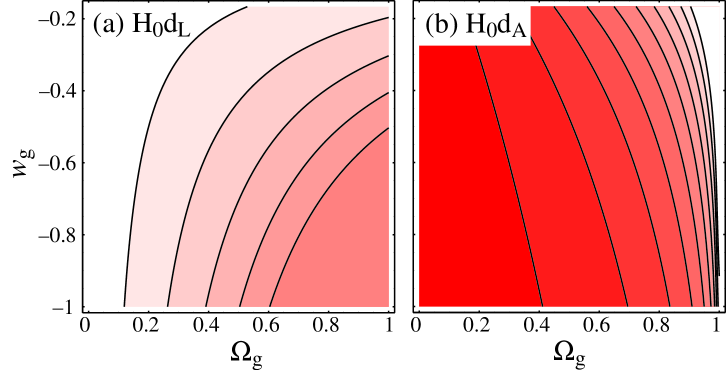
FIG. 1.: Distance measure degeneracies: contours of constant (a) luminosity distance to $z=0.5$ ($H_{0}d_{L}$) and (b) angular diameter distance to the last scattering surface ($H_{0}d_{A}$). $\Omega_{m}h^{2}$ has been held fixed in the former under the assumption that the CMB acoustic peak morphology will measure it independently. With this assumption, the two distance measures provide complementary information.

Isotropy demands that to lowest order the GDM stress tensor has only an isotropic (pressure) component. The GDM properties to lowest order therefore depend only on the equation of state $w_{g}=p_{g}/\rho_{g}$. For example, energy conservation requires that the evolution of the GDM density follows

$${d\ln\rho_{g}\over d\ln(1+z)^{-1}}=-3(1+w_{g})\,.$$ (1)

For simplicity, we consider models where $w_{g}$ is independent of the redshift $z$ since the properties of a slowly-varying $w_{g}$ can be modeled over the relevant redshifts with an appropriately weighted average [13, 21]. Combined with the assumption of zero spatial curvature, the expansion rate or Hubble parameter becomes

$${H\over H_{0}}(\Omega_{g},w_{g},\Omega_{m}/\Omega_{r};z)=[\Omega_{m}(1+z)^{3}+\Omega_{g}(1+z)^{3(1+w_{g})}+\Omega_{r}(1+z)^{4}]^{1/2}\,,$$ (2)

where $H_{0}=100\,h$ km s^-1 Mpc^-1. Here $\Omega_{m}=1-\Omega_{g}-\Omega_{r}$ and accounts for both the CDM and baryonic (“matter”) components. Likewise $\Omega_{r}$ accounts for the photon and neutrino (“radiation”) components. Furthermore, quantities that depend on the redshift behavior of the expansion rate such as the deceleration

$$q=-{(1+z)^{-1}\over H}{dH\over d(1+z)^{-1}}+1$$ (3)

depend on the same parameters. In particular, a component with $w_{g}<-1/3$ is able to drive $q$ negative and cause an acceleration.

Any cosmological observable that is simply a function of the expansion rate of the universe will only be sensitive to the background properties of the GDM through $(w_{g},\Omega_{g})$. For example, SN probe the luminosity distance (see Fig. 1a)

$$H_{0}d_{L}(w_{g},\Omega_{g};z)=(1+z)\int_{0}^{z}dz\,H_{0}/H\,;$$ (4)

this function is independent of the matter-radiation ratio because the observations are at sufficiently low redshift. Current SN luminosity distance data suggest the presence of an accelerating component with $w_{g}<-1/3$ (see Fig. 2) but may be dominated by unknown sources of systematic errors.

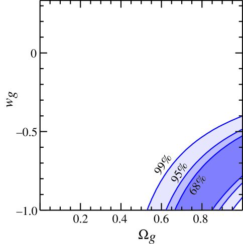
FIG. 2.: Current SN data. The 65%, 95% and 99% CL intervals in the $w_{g}-\Omega_{g}$ plane for the current data assuming only statistical errors. Constraints include 6 high redshift SN from the Supernova Cosmology Project [4] and 10 from the High-z Supernova Search [5]. We use 26 low-$z$ calibrating SN with $B-V<0.2$ obtained by the Calán/Tololo group [20]. The analysis follows [21], but note that systematic errors may dominate in the current data sets.

Likewise the acoustic peaks in the CMB probe the angular diameter distance to the redshift of last scattering $z_{\rm ls}$ (see Fig. 1b)

$$H_{0}d_{A}(w_{g},\Omega_{g},\Omega_{m}/\Omega_{r};z_{\rm ls})=\int_{0}^{z_{\rm ls}}dz\,H_{0}/H\,,$$ (5)

through its ratio with the sound horizon at last scattering $H_{0}s_{\rm CMB}(\Omega_{\gamma}/\Omega_{b},\Omega_{m}/\Omega_{r})$. Current CMB detections alone do not place significant on $w_{g}$ and $\Omega_{g}$ [21].

The energy density of the CMB is fixed through the measurement of its temperature $T_{\rm FIRAS}=2.728\pm 0.004$K (95% CL) [22] such that

$$\Omega_{\gamma}h^{2}=2.4815\times 10^{-5}\left({T_{\rm CMB}\over T_{\rm FIRAS}}\right)^{4}\,.$$ (6)

With this constraint, the dependence of the sound horizon on the photon-to-baryon ratio reduces to a dependence on $\Omega_{b}h^{2}$. Likewise, the total radiation energy density is given by

$$\Omega_{r}h^{2}=\Omega_{\gamma}h^{2}\left[1+0.681{N_{\nu}\over 3}\left(1.401T_{\nu}\over T_{\rm CMB}\right)^{4}\right]\,.$$ (7)

Thus under the usual assumptions for the number of neutrino species ($N_{\nu}=3$) and their thermal history ($T_{\nu}=T_{\rm CMB}/1.401$), the dependence of $d_{A}$ and $s_{\rm CMB}$ on $\Omega_{m}/\Omega_{r}$ becomes a dependence on $\Omega_{m}h^{2}$. We relax these assumptions in §VI to test the properties of the NBR.

B Structure Formation

To probe the remaining properties of the GDM, one must consider its effects on the gravitational instability of perturbations. Unless $w_{g}=-1$ (the cosmological constant case $\Omega_{g}=\Omega_{\Lambda}$), the GDM participates in the gravitational instability process. The cosmological constant case is special since the relativistic momentum density, which is proportional to $1+w_{g}$, goes to zero.

Since the perturbations need only be statistically isotropic, the GDM in general requires two parameters to describe fluctuations in its stress tensor. These can be chosen to be the sound speed in the rest frame of the GDM $c_{\rm eff}$, where $c^{2}_{\rm eff}\equiv\delta p_{g}/\delta\rho_{g}$ (in units of where $c=1$), which relates the pressure fluctuation to the density perturbation, and a “viscosity” parameter $c_{\rm vis}$, which relates velocity and metric shear to the anisotropic stress. See [8] for their precise covariant definition. Positive values of $c^{2}_{\rm eff}$ imply that density fluctuations are stabilized by pressure support at the effective sound horizon $s_{\rm eff}\equiv\int c_{\rm eff}(1+z)dt$. Likewise, positive values of $c^{2}_{\rm vis}$ imply that resistance to shearing stabilizes the fluctuation at $s_{\rm vis}\equiv\int c_{\rm vis}(1+z)dt$. These definitions assume that $c_{\rm eff}$ and $c_{\rm vis}$, respectively, are slowly varying. We call the greater of $s_{\rm eff}$ and $s_{\rm vis}$ the GDM sound horizon $s_{\rm GDM}$.

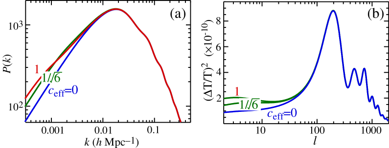
FIG. 3.: Sound speed effects for $w_{g}=-1/3$. A finite sound speed $c_{\rm eff}$ stabilizes perturbations leading to features in the (a) galaxy power spectrum and (b) CMB anisotropy spectrum. Note that in both cases the effects change most rapidly with $c_{\rm eff}$ between $0$ and $\sqrt{1/6}$. The power spectra have been normalized to small scales to bring out the degeneracies and the importance of large-scale information. The model here and throughout has $\Omega_{m}=0.35$, $h=0.65$, $\Omega_{b}h^{2}=0.02$, $\tau=0.05$, $n=1$, and $T/S=0$.

Modes smaller than $s_{\rm GDM}$ are stabilized by stress support. If the GDM also dominates the expansion rate then the growth of structure will slow below this scale. If $w_{g}<0$, GDM domination occurs at approximately

$$1+z_{g}\equiv\left({\Omega_{g}\over\Omega_{m}}\right)^{-1/3w_{g}}\,.$$ (8)

Thus we expect a feature in the matter power spectrum between $H_{0}s_{\rm GDM}(w_{g},\Omega_{g})$ at $z=z_{g}$ and $z=0$. Since below the sound horizon, the effect of GDM is to slow the growth of structure independent of scale, the determination of $c_{\rm eff}$ from measurements of the galaxy power spectrum depends crucially upon having data across this range of scales. In Fig. 3a, we show the effect of varying $c_{\rm eff}$ on the power spectrum for $w_{g}=-1/3$. The models have been normalized to small scales to bring out the scale-independence of the small-scale suppression. Given that the normalization is uncertain because of the unknown proportionality constant between the mass and galaxy power spectrum usually defined as $b^{2}$ where $b$ is the “bias”. the only direct information from galaxy surveys on $c_{\rm eff}$ comes from large scales. Notice the most rapid change with $c_{\rm eff}$ occurs for $c_{\rm eff}<\sqrt{1/6}$.

The location of the GDM sound horizon also affects CMB anisotropies. By halting the growth of structure, the GDM causes gravitational potential wells to decay below the sound horizon $s_{\rm GDM}$ at $z_{g}$. A changing gravitational potential imprints fluctuations on the CMB via differential gravitational redshifts whose sum is called the integrated Sachs-Wolfe (ISW) effect. However, if the sound horizon is much smaller than the particle horizon, the photons will traverse many wavelengths of the fluctuation as the potential decays. The cancellation of red and blue shifts destroys the effect. Thus the largest effect arises when $c_{\rm eff}\sim 1$ but varies strongly with $c_{\rm eff}$ only as it becomes less than $c_{\rm eff}\sim\sqrt{1/6}$. Unfortunately, subtle differences in this large-angle temperature signal around $c_{\rm eff}=1$ will be difficult to pin down given cosmic variance.

Because of the strong $c_{\rm eff}$-dependence of features in the CMB and galaxy survey power spectra for $c_{\rm eff}\lesssim\sqrt{1/6}$, tight lower limits can be placed on $c_{\rm eff}$ from the data even though models around $c_{\rm eff}=1$ cannot be distinguished. Furthermore, the amplitude of the features decreases sharply as $w_{g}\rightarrow-1$ since even clustering above the sound horizon vanishes in this limit. Constraints on the sound speed will thus only be possible if the equation of state of the GDM differs significantly from a cosmological constant.

Finally, the viscous term also causes the growth of structure to halt. However, it has an additional effect that makes it unique since anisotropic stresses enter directly in the Poisson equation that defines their relation to the gravitational potentials [8]. In Fig. 4, we show the effect of replacing the neutrinos with GDM of $c_{\rm vis}=\sqrt{1/3}$ and $0$ in the CMB. The former component models the neutrinos accurately and the latter shows that the anisotropic stress of the dark matter produces potentially observable effects in the CMB. We will exploit this effect to propose a means of detecting the anisotropies in the neutrino background radiation in §VI.

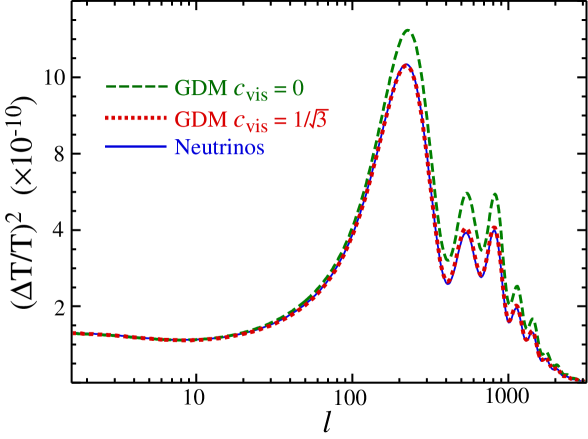
FIG. 4.: Viscosity effects: neutrinos may be accurately modeled as GDM with a viscosity parameter $c_{\rm vis}=\sqrt{1/3}$. Setting $c_{\rm vis}=0$ changes the CMB anisotropies significantly and equate to removing the quadrupole anisotropy of the NBR.

III Parameter Estimation

Projections for how well various data sets can measure cosmological parameters depend crucially on the extent of the parameter space considered as well as on the location in this space (or “fiducial model”) around which we quote our errors. Even though the latter uncertainty will be eliminated once the best fit model is found from the actual data, the former problem will remain. The extended GDM parameter space thus allows the data the freedom to choose the best values to describe properties of the dark sector. Even if the true model turns out to contain only conventional dark matter, it allows us to say with what confidence we can make this statement, i.e. that the dark components are in fact the neutrino background radiation, a cosmological constant, and cold dark matter. If these options are ruled out, then we will have discovered a new form of matter.

We adopt a 10-dimensional parameterization of cosmology that includes the present density of the GDM $\Omega_{g}$, a time-independent equation of state $w_{g}$, the matter density $\Omega_{m}h^{2}$, the baryon density $\Omega_{b}h^{2}$, the reionization optical depth $\tau$, the tilt $n$, the tensor-scalar ratio $T/S$, the normalization $A$, and the linear bias $b$. Both $c_{\rm eff}$ and $c_{\rm vis}$ affect the clustering scale and are largely degenerate. In §IV and §V, we take $c_{\rm eff}$ as a proxy for both, whereas in §VI, we take $c_{\rm vis}$ since we are interested in the anisotropy itself. This parameter space does not include models with non-zero spatial curvature or with massive neutrinos. We take the fiducial model to have $\Omega_{m}=1-\Omega_{g}=0.35$, $h=0.65$, $\Omega_{b}h^{2}=0.02$, $\tau=0.05$, $n=1$, and $T/S=0$; we will use fiducial models with different values of $w_{g}$ and $c_{\rm eff}$ to explore how the results depend on these parameters. For how the fiducial choices in the standard parameters affect the errors, see [3, 23].

To estimate errors on the cosmological parameters, we employ the Fisher matrix formalism (see [24] for a general review). The Fisher matrix is essentially an expansion of the log-likelihood function around its maximum in parameter space. It codifies the optimal errors on each parameter for a given experiment assuming a quadratic approximation for this function. Note that the Fisher matrix provides accurate estimates of error contours only when they encompass small variations in parameter space where the expansion is valid. This is an important caveat to which we will return in §V.

Fisher matrix errors thus employ derivatives of the cosmological observables with respect to parameters. To calculate derivatives of the CMB and galaxy power spectra, we employ the hierarchical Boltzmann code of [26, 27]. Special care must be taken in evaluating these derivatives since numerical noise in the calculation can artificially break any parameter degeneracies that exist. General techniques such as the taking of two-sided derivatives and the associated step sizes for standard parameters are described in [23]. For the GDM parameters, we estimate the derivatives by finite differences with the step sizes $\Delta\Omega_{g}=\pm 0.05(1-\Omega_{g})$, $\Delta w_{g}=\pm 0.01$, $\Delta c_{\rm eff}^{2}=\pm 0.1c_{\rm eff}^{2}$ and $\Delta c_{\rm vis}^{2}=\pm 0.1c_{\rm vis}^{2}$.

The benefit of a hierarchy treatment is that unlike the integral treatment of CMBfast [25], no interpolation is necessary and the code may be made arbitrarily accurate by adjusting the sampling in Fourier space. Thus the numerical noise problems identified by [23] can be addressed and in principle eliminated. However, computational speed generally requires a compromise involving smoothing the calculated CMB power spectrum [26]. We have tested our results against CMBfast version 2.3.2 in the context of flat $\Lambda$-models where CMBfast is most accurate and obtained $\sim 5\%$ agreement in parameter estimation with the hierarchy code. The test also involved two independent pipelines for taking model calculations through to parameter estimations. These comparisons were done with 1500 Fourier modes out to $k=2.5k_{\rm damp}$, where $k_{\rm damp}$ is the CMB damping scale (see [28], Eq. [17]) with Savitzky-Golay smoothing [29] of the resulting CMB angular power spectrum. We adopt the same techniques for parameter estimation in the GDM context.

In addition to the extent of the parameter space and the location of the fiducial model in parameter space, Fisher errors of course depend on the sensitivity of the given experiment. For the CMB data sets, we take the specifications of the MAP and Planck experiments given in [23]. We quote results with and without polarization information. Since the polarization signal may be dominated by foregrounds and systematic errors, the purely statistical Fisher matrix errors may be underestimates. For galaxy surveys, we take the Bright Red Galaxy sample of SDSS; the specifications and their translation into the Fisher matrix formalism is given in [30]. We further take the linear power spectrum for parameter estimation. Because non-linear effects and galaxy formation issues complicate the interpretation of the observed power spectrum on small scales, we employ information only from wavenumbers less than $k_{\rm max}=0.2h$Mpc^-1 and show how the results change as we go to a more conservative $k_{\rm max}=0.1h$Mpc^-1. This roughly brackets the regime where non-linear effects begin to play a role as shown by simulations [31]. For SN, we assume that on a timescale comparable to the MAP mission a total of $200$ supernovae will be found with individual magnitude errors of 0.3 and a redshift distribution with a mean of $z=0.65$ and a gaussian width of $\Delta z=0.3$ [32].

As each data set is independent to excellent approximation, the combined likelihood function is the product of the CMB, SN and galaxy survey likelihood functions. Thus the combined Fisher matrix is simply the sum of the individual Fisher matrices.

IV Measuring the Equation of State

Current SN luminosity distance measures suggest that the GDM may have an exotic equation of state $w_{g}\lesssim-1/3$ that accelerates the expansion (see Fig. 2 and [4, 5]). If these preliminary indications are borne out by future studies, one would like to pin down the equation of state of the GDM and also construct consistency tests to verify this explanation of the SN data. Unfortunately, no one data set can isolate the equation of state on its own. The CMB has one measure of $w_{g}$ from the angular diameter distance to the last scattering surface (see Eq. [5]), but this is degenerate with $\Omega_{g}$ (see Fig. 1), even assuming zero curvature and that $\Omega_{m}h^{2}$ has been measured from the morphology of the acoustic peaks. Leverage on $w_{g}$ and $\Omega_{g}$ comes only through the cosmic-variance-limited ISW effect at large angles and through the effects of gravitational lensing on very small scales. The latter occurs because changing $\Omega_{g}$ affects the present-day normalization of the matter power spectrum and thereby changes the amount of lensing. The effect is small, however, and much less powerful for breaking the degeneracy than the methods of the next paragraph; we therefore neglect lensing in the CMB. Likewise, galaxy surveys alone give leverage only through the combination that defines the GDM sound horizon. For SN measurements that span only a short range in redshift, there is an analogous degeneracy between $w_{g}$ and $\Omega_{g}$ in the luminosity distance (see Eq. [4]).

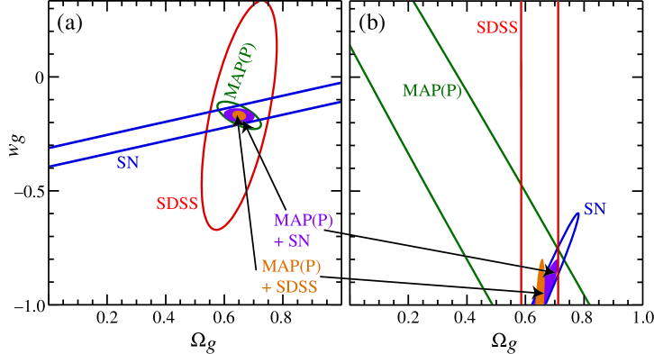
FIG. 5.: Breaking the equation-of-state density degeneracy. The degeneracy exposed in Fig. 1 can be broken by combining CMB information (here from MAP) with SN or galaxy survey (here from SDSS) information. Plotted here are the 68% CL for the various experiments and combinations. Comparison of the two combinations leads to a sharp consistency test. Two fiducial models are shown: (a) $w_{g}=-1/6$ and (b) $w_{g}=-1$. While the CMB alone does well at $w_{g}=-1/6$, its degeneracy worsens considerably as $w_{g}$ decreases toward $-1$. Note, however, that the complementary nature of the data sets and the ability to make consistency checks occurs in both cases.

However, combining two of these measurements isolates $w_{g}$ and the third can be used as a consistency check. That the CMB angular diameter distance and SN luminosity distance measures break each others degeneracies is obvious from comparing panels (a) and (b) in Fig. 1. We show in Fig. 5 the error ellipses (68% CL) in the $\Omega_{g}-w_{g}$ plane.

Due to the large ISW effect in the $w_{g}=-1/6$ model of Fig. 5a, MAP alone will provide reasonable constraints on the two parameters. In this case, SN measurements will provide a strong consistency check on CMB measurements. However, as one approaches $w_{g}=-1$, the ISW effect decreases and the CMB requires the assistance of SN measurements to break the degeneracy. We list the 1$\sigma$ errors as a function of $w_{g}$ in Tab. I.

The combination of CMB and galaxy survey data provides a more subtle example of complementarity. Despite the fact that the MAP error ellipse lies wholely within the SDSS error ellipse in Fig. 5a, the addition of SDSS provides substantially smaller error bars. As discussed in [34], the combination of the CMB and galaxy power spectrum information yields a precise measurement of the Hubble constant $h$ and $\Omega_{m}$ independently of any low redshift GDM effects. The reason is that the physical extent of the sound horizon at recombination can be precisely calibrated from measurement of $\Omega_{b}h^{2}$ and $\Omega_{m}h^{2}$ through the acoustic peak morphology (see Fig. 6 and [35]). Measurement of this scale in redshift space isolates the Hubble constant; the aforementioned measurement of $\Omega_{m}h^{2}$ in the CMB then returns $\Omega_{m}$. Under the assumption of a flat universe, $\Omega_{g}=1-\Omega_{m}$ is also well determined (see Fig. 5b) and the angular diameter distance $d_{A}(\Omega_{m}h^{2},\Omega_{g},w_{g})$ may be used to extract $w_{g}$. Hence, despite the fact that galaxy surveys cannot determine these parameters by themselves, they can break the angular diameter distance degeneracy of the CMB and thereby allow the CMB to measure $w_{g}$ and $\Omega_{g}$. The subtle nature of the degeneracy breaking requires a full joint analysis to uncover (c.f. [9] who reached more pessimistic conclusions from a separate examination of each data set).

If the measurements pass the consistency test, we can combine all three sets of data. Even assuming no polarization information from MAP, the result is that the errors on $w_{g}$ in the worst case of $w_{g}=-1$ become $\sigma(w_{g})=0.056$, allowing for a sharp test for the presence of a cosmological constant. Failure to achieve consistency would indicate that one of our assumptions is wrong, e.g. $w_{g}$ varies strongly with time or spatial curvature does not vanish $\Omega_{g}\neq 1-\Omega_{m}$.

Finally, note that by marginalizing $c_{\rm eff}$, our results treat the clustering properties of the GDM as unknown and are thus conservative in the context of scalar-field quintessence models [33]. For example if $c_{\rm eff}$ is held fixed, the limits on $w_{g}$ for the $w_{g}=-1/6$ model improve by $\sim 30\%$ for MAP+SDSS with or without polarization; gains are negligible near $w_{g}=-1$ since $c_{\rm eff}$ has little observable effect there.

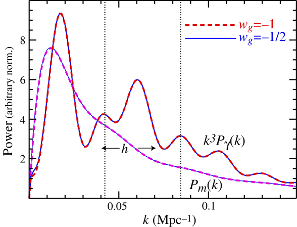
FIG. 6.: Measurement of $h$ and the equation of state degeneracy. Acoustic features in both the CMB ($k^{3}P_{\gamma}$) and matter/galaxy power ($P_{m}$) spectra are frozen in at last scattering. Once the CMB acoustic peaks are calibrated in real space from the peak morphology measurement of $\Omega_{m}h^{2}$ and $\Omega_{b}h^{2}$, sliding the galaxy power spectrum in redshift space ($h$ Mpc^-1) until the features “match” determines $h$. This test is unaffected by and therefore insensitive to late-time dynamics from the GDM component. However, once $h$ is determined, $\Omega_{g}=1-\Omega_{m}$ follows from the CMB measurement of $\Omega_{m}h^{2}$. The angular diameter distance measurement from the CMB then determines $w_{g}$.

In summary, for any value of $w_{g}$, the combination of CMB data with SN distance measures or galaxy surveys will provide reasonably precise measures of $w_{g}$ and $\Omega_{g}$ even considering the unknown clustering properties of the GDM. The comparison of these two combinations provides a sharp consistency test.

$c_{\rm eff}=0.03$	MAP(P)+SDSS		MAP(P)+SN		Planck(P)+SDSS		Planck(P)+SN
$w_{g}$	$\sigma(w_{g})$	$\sigma(\Omega_{g})$	$\sigma(w_{g})$	$\sigma(\Omega_{g})$	$\sigma(w_{g})$	$\sigma(\Omega_{g})$	$\sigma(w_{g})$	$\sigma(\Omega_{g})$
-1/6	0.015 (0.033)	0.017 (0.028)	0.024	0.030	0.009 (0.014)	0.007 (0.010)	0.014	0.009
-1/3	0.027 (0.056)	0.013 (0.022)	0.028	0.031	0.016 (0.029)	0.010 (0.019)	0.020	0.013
-1/2	0.047 (0.088)	0.013 (0.022)	0.041	0.034	0.022 (0.041)	0.010 (0.019)	0.021	0.011
-2/3	0.074 (0.129)	0.013 (0.022)	0.063	0.037	0.029 (0.052)	0.010 (0.020)	0.023	0.010
-5/6	0.108 (0.183)	0.013 (0.022)	0.091	0.040	0.037 (0.064)	0.010 (0.019)	0.026	0.009
-1	0.126 (0.201)	0.011 (0.018)	0.125	0.042	0.033 (0.050)	0.008 (0.016)	0.027	0.010

TABLE I.: Errors on $w_{g}$ and $\Omega_{g}$ upon combining data sets. SDSS assumes information out to $k_{\rm max}=0.2h$Mpc^-1 or $0.1h$Mpc^-1 (parentheses). For $w_{g}<-1/6$, errors are insensitive to the sound speed of the fiducial model; here we use $c_{\rm eff}=\sqrt{0.03}\approx 0.2$.

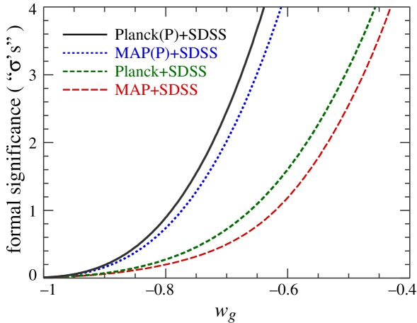
FIG. 7.: Significance of bounds on $c_{\rm eff}$ as a function of the equation of state $w_{g}$ of the fiducial model. Plotted is the formal significance with which the simplest scalar-field models ($c_{\rm eff}=1$) may be excluded if the true model is $c_{\rm eff}=\sqrt{0.03}\sim 0.2$. The formal errors may overestimate the significance as discussed in the text. The power to distinguish sound speed effects decreases sharply as one approaches the cosmological constant case of $w_{g}=-1$.

V Constraining the Sound Speed

If the tests of the last section determine that the equation of state of the exotic component is in the range $-1<w_{g}<0$, we will have discovered a new form of matter. It then becomes interesting to explore its properties in order to search for a suitable particle physics candidate. The simplest candidate is a slowly-rolling scalar field, also known as “quintessence” [10, 11, 12, 13]. The hallmark of such a candidate is that its effective sound speed is simply the speed of light ($c_{\rm eff}=1$), i.e. it is a maximally stable form of matter. It furthermore has $c_{\rm vis}=0$. Can the clustering properties of the GDM be measured well enough to distinguish a scalar field component from alternate candidates for the exotic matter?

Stabilization of perturbations may occur through a finite effective sound speed $c_{\rm eff}$ as it does for a real scalar field or through viscosity $c_{\rm vis}$ as some defect-dominated models suggest [17, 18]. Because the two are largely degenerate, we take $c_{\rm eff}$ as a proxy for both – one actually determines the combination of $c_{\rm eff}$ and $c_{\rm vis}$ that fixes the GDM sound horizon.

The sound speed $c_{\rm eff}$ will only be well constrained if the GDM sound horizon at $z_{g}$ is sufficiently small that cancellation of the ISW effect varies strongly with $c_{\rm eff}$ (see Fig. 3) or if the features in the matter power spectrum lie on scales accessible to galaxy surveys. Both of these considerations favor fiducial models with low $c_{\rm eff}$. SN distance measures have no dependence on $c_{\rm eff}$. In Table II (upper), we show the errors on $c_{\rm eff}$ as its fiducial value increases in an $w_{g}=-1/3$, $\Omega_{g}=0.65$ fiducial model. As usual, both these and other parameters are marginalized when quoting errors on $c_{\rm eff}^{2}$. As expected, the error $\sigma(c_{\rm eff}^{2})$ increases sharply as $c_{\rm eff}\rightarrow 1$.

The strong variation of $\sigma(c_{\rm eff}^{2})$ with $c_{\rm eff}^{2}$ itself makes it difficult to estimate the significance at which two models can be separated. For example, if we were to take $\sigma(c_{\rm eff}^{2}=0.3)$ to infer that it is distinguishable from $c_{\rm eff}^{2}=0$ at only $0.3/1.52=0.2\sigma$ from MAP+SDSS, we would be incorrect since a model with a smaller value $c_{\rm eff}^{2}=0.03$ is distinguishable from zero at a higher level. Conversely, the ability to distinguish a fiducial model with $c_{\rm eff}=0$ from one with $c_{\rm eff}>0$ is always overestimated. This problem reflects the limitations of the Fisher matrix technique caused by its infinitesimal expansion of the likelihood function.

To address this issue, we take an intermediate value of $c_{\rm eff}=\sqrt{0.03}\sim 0.2$ and ask how well we can reject the scalar field hypothesis of $c_{\rm eff}=1$. We plot in Fig. 7, the number of standard deviations by which the true sound speed is separated from the scalar field value [“$\sigma$’s” $=(1-c_{\rm eff}^{2})/\sigma(c_{\rm eff}^{2})]$. Although this formal significance still overestimates the true significance, the qualitative result is clear. If $w_{g}\gtrsim-1/2$, CMB and galaxy survey data will be able to place interesting constraints on the sound speed. As $w_{g}$ decreases to $-1$, the effects of clustering in the GDM vanish leaving no significant constraint on $c_{\rm eff}$. A more complete exploration of the likelihood function would yield more precise limits but is computationally time consuming; we defer such an analysis until $w_{g}$ is measured and shown to be in this range.

$c_{\rm eff}^{2}$	$\sigma(c_{\rm eff}^{2})$
no priors:	MAP+SDSS	MAP(P)+SDSS	Planck+SDSS	Planck(P)+SDSS
0.03	0.13 (0.13)	0.06 (0.06)	0.12 (0.12)	0.04 (0.04)
0.1	0.46 (0.47)	0.14 (0.15)	0.42 (0.43)	0.10 (0.10)
0.3	1.52 (1.55)	0.54 (0.54)	1.47 (1.47)	0.37 (0.37)
$\sigma(\ln\beta)=0.1$:
0.03	0.06 (0.06)	0.06 (0.06)	0.06 (0.06)	0.04 (0.04)
0.1	0.18 (0.20)	0.14 (0.15)	0.18 (0.18)	0.10 (0.10)
0.3	0.75 (0.83)	0.52 (0.53)	0.72 (0.72)	0.37 (0.38)

TABLE II.: Errors on $c_{\rm eff}^{2}$ as a function of its fiducial value for $w_{g}=-1/3$. SDSS assumes $k_{\rm max}=0.2h$ Mpc^-1 ($0.1h$ Mpc^-1). P denotes the inclusion of CMB polarization information. Upper: no priors on $\beta$; lower: prior of $\sigma(\ln\beta)=0.1$. The prior helps isolate $\tau$ if polarization information is unavailable and hence brings the limits with and without polarization closer.

Fig. 7 implies that good limits on $c_{\rm eff}$ depend on polarization information. This is because reionization effects are nearly degenerate with ISW effects from $c_{\rm eff}$. We show this in Fig. 8. Polarization information isolates $\tau$ from the feature generated by Thomson scattering of anisotropic radiation present at large scales during reionization. However, because of foregrounds and systematics likely in the large-angle polarization data, it is interesting to see whether any other information can break this degeneracy. The main effect of $\tau$ is to reduce the small-angle anisotropies in the CMB uniformly. If the intrinsic amplitude can be calibrated by the galaxy survey data, $\tau$ could be measured. With the growth function and other transfer function effects under control, the remaining obstacle is the unknown bias factor $b$. This can be measured on large scales through redshift-space distortions. Since $\Omega_{m}$ is well-constrained by the combination of CMB and galaxy survey data (§ IV), the constraint on $\beta=\Omega_{m}^{0.6}/b$ from these distortions supply information on the bias. Taking a conservative prior of $\sigma(\ln\beta)=0.1$ [36], the normalization determination breaks the $c_{\rm eff}^{2}-\tau$ degeneracy almost as effectively as polarization information. We quantify this in Tab. II (lower), where the errors on $c_{\rm eff}^{2}$ with and without polarization are made more comparable with this conservative prior on $\beta$.

In summary, interesting constraints on the clustering properties of the exotic component will be available if $w_{g}\gtrsim-1/2$ as long as we have either polarization data from the CMB or redshift-space distortion information from galaxy surveys.

FIG. 8.: The $\tau-c_{\rm eff}^{2}$ degeneracy. $\tau$ and $c_{\rm eff}^{2}$ are nearly degenerate given only temperature information. With either polarization information on the CMB side [MAP(P)] or a prior of $\sigma(\ln\beta)=0.1$ from redshift space distortions on the galaxy power spectrum side [SDSS($\beta$)], the degeneracy is broken allowing better isolation of $c_{\rm eff}^{2}$.

VI Detecting the Neutrino Background Radiation

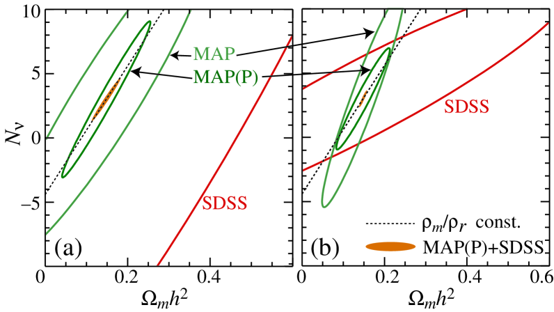
FIG. 9.: Matter-Radiation degeneracy. Plotted here are the 68% CL for the various experiments. (a) Ignoring the information supplied by the anisotropy of the NBR by marginalizing over $c_{\rm vis}$, we find a strong degeneracy between the neutrino number $N_{\nu}$ and the matter density $\Omega_{m}h^{2}$ along a line of constant matter-radiation ratio $\rho_{m}/\rho_{r}$ in both the CMB and galaxy survey data. Combining CMB information from MAP and galaxy information from SDSS breaks the degeneracy somewhat. (b) Utilizing the information in the anisotropies by assuming $c_{\rm vis}=\sqrt{1/3}$ shrinks and rotates the error ellipses leading to better complementarity and tighter errors.

If the equation of state of the GDM is determined to be $w_{g}=-1$, then the only possibility is a cosmological constant. In this case, the basic aspects of structure formation are so simple that subtle effects in the dark sector can be uncovered. The remaining dark matter in the universe is the neutrino background radiation (NBR). How well can we detect its presence? The issue is somewhat more subtle than it initially appears due to a degeneracy in the CMB acoustic peaks. We shall see that detecting the neutrino background radiation requires detecting its fluctuations, in particular its anisotropies.

A Matter-Radiation Degeneracy

Given that CMB anisotropies are generally sensitive to changes in the expansion rate at high redshift, one might think the radiation content of the universe could be measured precisely. Indeed the matter density $\Omega_{m}h^{2}$ can be measured to $\sigma(\Omega_{m}h^{2})=0.02$ by the MAP satellite (without polarization) if the radiation is taken to be fixed. The problem is that what the CMB best measures is the matter-radiation ratio, not the matter or radiation density individually.

The GDM parameterization can be used to explore this degeneracy and more generally deconstruct the information contained about the NBR in the CMB. We know that the matter-radiation degeneracy arises because of the way the background expansion rate scales with these parameters [see Eq. (2)]. Fluctuations in the matter and radiation break this degeneracy. We can use the GDM parameterization to separate the information on the background expansion rate from that of the fluctuation properties.

As shown in §II and [8], the NBR is accurately modeled by a GDM component with $w_{g}=c_{\rm eff}^{2}=c_{\rm vis}^{2}=1/3$ and density $\Omega_{g}=5.63\times 10^{-6}h^{-2}N_{\nu}$. $N_{\nu}=3$ in the fiducial model. Thus $N_{\nu}$ and $w_{g}$ determine the background properties whereas $c_{\rm eff}$ and $c_{\rm vis}$ control the fluctuation properties, with $c_{\rm vis}$ controlling the anisotropic stress of the NBR. The anisotropic stress is proportional to the quadrupole anisotropy of the NBR. Thus $c_{\rm vis}=0$ (with $c_{\rm eff}=\sqrt{1/3}$) represents a component with the same background properties as the NBR but with no anisotropies.

How does ignorance of the properties of the NBR affect the determination of the matter density $\Omega_{m}h^{2}$? If we allow $N_{\nu}$ and $c_{\rm vis}$ to vary so as to eliminate the information provided by the density and anisotropy of the radiation component, the error ellipses of Fig. 9a reveal a matter-radiation degeneracy, i.e. they are elongated along the line of constant matter-radiation density ratio. The degeneracy affects both CMB measurements and galaxy surveys alike. Here and in the remainder of this section, we keep $w_{g}$ and $c_{\rm eff}$ fixed while varying $\Omega_{g}$, $c_{\rm vis}$, and the other cosmological parameters including a cosmological constant $\Omega_{\Lambda}$. The MAP errors on $\Omega_{m}h^{2}$ are degraded from $\sigma(\Omega_{m}h^{2})=0.02$ to $0.16$ when $N_{\nu}$ is allowed to vary. The baryon-to-photon ratio $\Omega_{b}h^{2}$ remains well-measured. Some leverage in a flat universe is provided by the fact that the actual matter density comes into the angular diameter distance for the CMB. Indeed, if one fixes the other parameters that go into the angular diameter distance, in this context $\Omega_{\Lambda}$, then the CMB does place tight constraints on $\Omega_{m}h^{2}$ and $N_{\nu}$ separately [38]. However, in the general case, the angular diameter distance degeneracy prevents a precise measurement of $\Omega_{m}h^{2}$ by these means.

Combining CMB anisotropies and galaxy power spectrum information, which both suffer from the matter-radiation degeneracy individually, restores tight error bars on $\Omega_{m}h^{2}$ even using only temperature information from MAP (see Tab. III). Here the additional information on $\Omega_{b}/\Omega_{m}$ from baryonic features in the galaxy power spectrum along with the precise measurement of $\Omega_{b}h^{2}$ from the CMB constrains $\Omega_{m}h^{2}$. This is another example in which the complementary nature of the CMB and galaxy survey data helps in a subtle way.

B Limiting the Number of Neutrinos

In the standard scenario, the fluctuations of the NBR are not unknown; they are fixed through the properties of the neutrinos and gravitational instability. These fluctuations in the NBR further breaks the matter-radiation degeneracy. Like the CMB itself, the NBR carries temperature anisotropies (see [26] for the full angular power spectrum). In particular, the quadrupole anisotropy of neutrinos alters the gravitational potentials that drive acoustic oscillations (see Fig. 4).

By fixing $c_{\rm vis}=\sqrt{1/3}$, we can ask how well the number $N_{\nu}$ of neutrino species in the NBR can be measured under the standard assumptions. This is appropriate for either flavored or sterile neutrinos if their mass is sufficiently small ($m_{\nu}\lesssim 0.1$ eV). We show the results in Fig. 9b and Tab. III. The CMB and galaxy survey ellipses in the $N_{\nu}$–$\Omega_{m}h^{2}$ plane shrink and rotate in opposite senses from the case of a marginalized $c_{\rm vis}$ (Fig. 9a). This enhances the complementary nature of CMB and galaxy survey data giving a substantial improvement when the data sets are combined if only MAP data is available.

As the errors in Tab. III are comparable to those achievable from big bang nucleosynthesis (BBN) [40], CMB and galaxy surveys should provide a powerful consistency check on BBN and a constraint on additional neutrino species populated around recombination. Unfortunately, testing percent-level differences in the NBR temperature (represented here by a change $\delta N_{\nu}/N_{\nu}=4\delta T_{\nu}/T_{\nu}$, see Eq. [7]) due to the details of their decoupling [37, 38, 39] seems out of reach even if we combine all of our precision tests.

	MAP+SDSS		MAP(P)+SDSS		Planck+SDSS		Planck(P)+SDSS
assumption	$\sigma(\Omega_{m}h^{2})$	$\sigma(N_{\nu})$	$\sigma(\Omega_{m}h^{2})$	$\sigma(N_{\nu})$	$\sigma(\Omega_{m}h^{2})$	$\sigma(N_{\nu})$	$\sigma(\Omega_{m}h^{2})$	$\sigma(N_{\nu})$
unknown $c_{\rm vis}^{2}$	0.026 (0.046)	1.24 (2.26)	0.023 (0.036)	1.12 (1.92)	0.006 (0.006)	0.30 (0.43)	0.004 (0.004)	0.21 (0.23)
fixed $c_{\rm vis}^{2}$	0.007 (0.024)	0.44 (1.59)	0.006 (0.022)	0.43 (1.44)	0.003 (0.005)	0.23 (0.43)	0.003 (0.003)	0.17 (0.20)

TABLE III.: Errors on $\Omega_{m}h^{2}$ and $N_{\nu}$ with and without information from NBR anisotropies. SDSS assumes $k_{\rm max}=0.2h$ Mpc^-1 ($k_{\rm max}=0.1h$ Mpc^-1). P denotes the inclusion of CMB polarization information.

C Detecting Neutrino Anisotropies

Anisotropies in the NBR are predicted by the gravitational instability paradigm and are potentially observable through their effect on CMB anisotropies. In the GDM model for the NBR, the anisotropies are determined by the viscosity parameter $c_{\rm vis}$; constraints on this parameter tell us how well anisotropies in the NBR can be detected. The role of the viscosity parameter $c_{\rm vis}$ in breaking degeneracies in the last section suggests that the anisotropies in the neutrino background radiation may themselves be detectable. Unfortunately, with the CMB alone, the effect is strongly degenerate with those of other parameters. Even though we fix the other properties of the GDM ($w_{g}=c_{\rm eff}^{2}=1/3$, $N_{\nu}=3$), changes in $c_{\rm vis}$ can be mimicked by changes in the normalization and tilt of the spectrum at small angles.

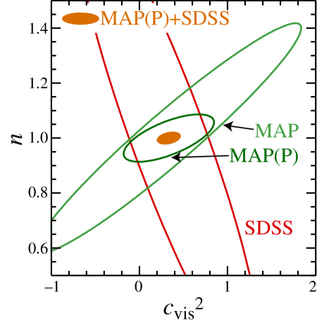
FIG. 10.: Detecting anisotropies in the neutrino background radiation. Anisotropies in the NBR are detectable if a model with $c_{\rm vis}^{2}=1/3$ can be distinguished from one with $c_{\rm vis}^{2}=0$. Degeneracy with other parameters such as the tilt $n$ prevent the CMB information provided by MAP from detecting the anisotropies. Adding galaxy survey information from SDSS breaks the degeneracy and allows a statistically significant detection. We have assumed here that $N_{\nu}$ is fixed at 3.

By adding in galaxy survey data, $c_{\rm vis}^{2}=1/3$ (NBR anisotropies) and $c_{\rm vis}^{2}=0$ (no anisotropies) are separated by $3.5\sigma$ from MAP+SDSS. The significance improves to 8.7$\sigma$ with Planck.

How sensitive is the measurement to the underlying assumptions about the data set and model space? The loss of polarization information does not significantly affect these limits. On the other hand, if we take the more conservative $k_{\rm max}=0.1h$Mpc^-1 for the galaxy surveys, the significance decreases to $1.2\sigma$ ($7.3\sigma$) for MAP+SDSS (Planck+SDSS). Perhaps more important, the MAP+SDSS result does depend on prior knowledge that $N_{\nu}\approx 3$. Fortunately, even assuming only very conservative constraints of $\sigma(N_{\nu})=1.0$ from big bang nucleosynthesis, allows a detection at 2.0$\sigma$ (7.1$\sigma$) for MAP+SDSS (Planck+SDSS). These results imply that NBR anisotropies can be detected with high significance at least by the Planck satellite, even under conservative assumptions.

VII Conclusions

With the wealth of precision cosmological measures that are becoming available, we should soon be in the position to identify all of the cosmologically important components of the universe – including any dark components that may be present. Not only do CMB anisotropies, high-redshift objects, and galaxy surveys probe different aspects of the cosmology, but they can work together to uncover a complete and consistent cosmological picture.

We have shown here how the combined power of these data sets can determine the properties of the dark components. Assuming that the preliminary indications from SN data that the missing component is not merely spatial curvature are confirmed, the first step will be to determine the equation of state of the exotic component. The task is non-trivial due to a degeneracy with its density in determining the expansion rate. The degeneracy is broken by combining the CMB data with SN distance measures, galaxy surveys, or any other measurement that can constrain $\Omega_{m}=1-\Omega_{g}$ or $h$. By further combining any of these pairs of data sets, we create powerful consistency tests. Note that these tests work even near a cosmological constant model $p_{g}/\rho_{g}\equiv w_{g}=-1$, where the degeneracy in the CMB alone is at its worst.

Should the equation-of-state measurement rule out a cosmological constant, we will want to study the other properties that identify this exotic component. Its clustering scale is accessible in the CMB and galaxy surveys as features in their power spectra at large scales. We have parameterized this with a sound speed and have shown that as long as the equation of state is sufficiently different from a cosmological constant ($w_{g}\gtrsim-1/2$), one can distinguish a maximally stable component ($c_{\rm eff}=1$) from a component with $c_{\rm eff}\lesssim 0.2$. Distinguishability increases substantially as $p_{g}/\rho_{g}$ increases, reaching $c_{\rm eff}\lesssim 0.6$ at $w_{g}=-1/6$. Such limits are interesting since the simplest physically motivated exotic component, a slowly-rolling scalar-field quintessence, is maximally stable with $c_{\rm eff}=1$.

We have only considered models where the equation of state varies in time sufficiently slowly to be replaced by some suitably averaged but constant $w_{g}$. If the GDM sector involves stronger temporal variation, to what extent will upcoming data sets be able to constrain the possibilities? As noted in §IV, acoustic features in the CMB anisotropies when combined with those in the galaxy power spectrum can be combined to measure $\Omega_{m}$. This measurement requires that the dark components at high redshift such as the NBR are known but makes no assumptions whatsoever about the low-redshift behavior of $w_{g}$. With the present-day value of $\Omega_{g}=1-\Omega_{m}$ known to fair accuracy, there are a number of observational handles on $w_{g}$ as a function of time. The location of the CMB acoustic peaks determines the angular diameter distance to high redshift. Mid-redshift supernovae constrain the luminosity distance to $z\approx 0.5$, although with very large samples one may even extract some redshift dependence. Measurements of the normalization of the power spectrum on scales below the GDM sound horizon will constrain the GDM-modified growth rate. The $z=0$ normalization may be measured from abundances of rich clusters [41] and from the galaxy power spectrum given a measurement of galaxy bias from redshift distortions or peculiar velocity data sets. The normalization at higher redshift can be estimated from the statistics of the Lyman $\alpha$ forest, damped Lyman $\alpha$ systems, and high-redshift clusters. Hence, although the most general equation of state is described by a free function of redshift, there are actually a number of robust observational handles on its behavior!

A similar analysis shows that even if the universe contains both an accelerating component and a non-vanishing spatial curvature, which in many respects resembles a universe with $w_{g}$ varying from $-1/3$ to $-1$, the combination of information from different redshifts will give us leverage on the two separately. The situation is actually even more favorable since the geometrical aspects of curvature enter strongly into the angular diameter distance as measured by the CMB.

Should the measurement of the equation of state confirm the relative simplicity of a cosmological constant, we will be able to probe in detail the remaining dark component, the neutrino background radiation. Detection of the neutrino background radiation through the CMB suffers from the fact that a change its energy density may be compensated with a change in the matter density up to effects due to the presence of fluctuations. We have shown that by combining CMB and galaxy survey data, this degeneracy can be broken and yields constraints competitive with those from big bang nucleosynthesis. Furthermore, the combination of CMB and galaxy survey data should provide the first detection of anisotropies in the neutrino background radiation. The detection of these anisotropies, predicted by the gravitational instability paradigm for structure formation, would represent a triumph for cosmology.

Acknowledgements: W.H. is supported by the Keck Foundation and a Sloan Fellowship, W.H. and D.J.E. by NSF-9513835, D.J.E. by a Frank and Peggy Taplin Membership at the IAS, and M.T. by NASA through grant NAG5-6034 and Hubble Fellowship HF-01084.01-96A from STScI, operated by AURA, Inc. under NASA contract NAS4-26555.

REFERENCES

- [1] MAP: http://map.gsfc.nasa.gov
- [2] Planck: http://astro.estec.esa.nl/SA-general/Projects/Planck
- [3] G. Jungman, M. Kamionkowski, A. Kosowsky, & D. N. Spergel, Phys. Rev. D 54, 1332 (1996) [astro-ph/9512139]; J.R. Bond, G. Efstathiou, & M. Tegmark, Mon. Not. Roy. Astr. Soc. 291, L33 (1997) [astro-ph/9702100]; M. Zaldarriaga, D. N. Spergel, & U. Seljak, Astrophys. J. 488, 1 (1997) [astro-ph/9702157]
- [4] S. Perlmutter, et al., Astrophys. J. 483, 565 (1997) [astro-ph/9608192]; S. Perlmutter, et al. Nature (London) 391, 51 (1998)
- [5] P. M. Garnavich, et al., Astrophys. J. Lett 493, 53 (1998) [astro-ph/9710123]; A. G. Riess, et al., preprint [astro-ph/9805201]
- [6] 2dF: http://meteor.anu.edu.au/colless/2dF
- [7] SDSS: http://www.astro.princeton.edu/BBOOK
- [8] W. Hu, Astrophys. J. (to be published) [astro-ph/9801234]
- [9] G. Huey, L. Wang, R. Dave, R.R. Caldwell, & P. J. Steinhardt, preprint [astro-ph/9804285]
- [10] B. Ratra & P. J. E. Peebles, Phys. Rev. D. 37, 3406 (1988); P. J. E. Peebles & B. Ratra, Astrophys. J. 325, L17 (1988)
- [11] N. Sugiyama & K. Sato, Phys. Rev. D. 387, 439 (1992)
- [12] J. A. Frieman, C. T. Hill, A. Stebbins, & I. Waga, Phys. Rev. Lett. 75, 2077 (1995) [astro-ph/9505060]; K. Coble, S. Dodelson, & J. Frieman, Phys. Rev. D 55, 1851 (1997) [astro-ph/9608122]; J. A. Frieman & I. Waga, Phys. Rev. D 57, 4642 (1998) [astro-ph/9709063]
- [13] R. R. Caldwell, R. Dave, & P. J. Steinhardt, Phys. Rev. Lett. 80 1582 (1998) [astro-ph/9708069]; R. R. Caldwell & P. J. Steinhardt, Phys. Rev. D. 57, 6057 (1998) [astro-ph/9710062]
- [14] H. Kodama & M. Sasaki, M. Prog. Theor. Phys. Supp. 78, 1 (1984)
- [15] T. Chiba, N. Sugiyama, & T. Nakamura, Mon. Not. Roy. Astr. Soc. 289 5 (1997) [astro-ph/9704199]; T. Chiba, N. Sugiyama, & T. Nakamura, preprint [astro-ph/9806332]
- [16] M. S. Turner & M. White, Phys. Rev. D. 56, 4439 (1997) [astro-ph/9701138]
- [17] D. N. Spergel & U.-L. Pen, Astrophys. J. Lett. 491, L67 (1997) [astro-ph/9611198]
- [18] M. Bucher, private communication
- [19] N. Turok, U.-L. Pen, & U. Seljak, preprint [astro-ph/9706250]
- [20] M. Hamuy, et al., Astronomical J. 112, 2398 (1996) [astro-ph/9609064]
- [21] M. White, Astrophys. J. (to be published) [astro-ph/9802295]
- [22] D. Fixsen, et al. Astrophys. J. 473, 576 (1996) [astro-ph/9605054]
- [23] D. J. Eisenstein, W. Hu, & M. Tegmark, Astrophys. J. (submitted)
- [24] M. Tegmark, A. N. Taylor, & A. F. Heavens, Astrophys. J. 480, 22 (1997) [astro-ph/9603021]
- [25] U. Seljak & M. Zaldarriaga, Astrophys. J. 469 437 (1996) [astro-ph/9603033]
- [26] W. Hu, D. Scott, N. Sugiyama, & M. White, Phys. Rev. D. 52, 5498 (1995) [astro-ph/9505043]
- [27] M. White & D. Scott, Astrophys. J. 459, 415 (1996) [astro-ph/9508157]
- [28] W. Hu & M. White, Astrophys. J. 479, 568 (1997) [astro-ph/9609079]
- [29] W. H. Press, S. A. Teukolsky, W. T. Vetterling, & B. P. Flannery, Numerical Recipes in Fortran, Second Edition (Cambridge University Press, New York, 1992)
- [30] M. Tegmark, Phys. Rev. Lett. 79, 3806 (1997) [astro-ph/9706198]
- [31] A. Meiksen, M. White, & J. Peacock (in preparation)
- [32] M. Tegmark, D. J. Eisenstein, W. Hu, & R. Kron, preprint [astro-ph/9805117]
- [33] M. White (in preparation)
- [34] D. J. Eisenstein, W. Hu, & M. Tegmark, preprint [astro-ph/9805239]
- [35] W. Hu & M. White, Astrophys. J. 471, 30 (1996) [astro-ph/9602019]
- [36] S. Hatton & S. Cole, Mon. Not. Roy. Astron. Soc. 296, 10 (1998) [astro-ph/9707186]
- [37] S. Dodelson & M. Turner, Phys. Rev. D. 46, 3372 (1992)
- [38] R. E. Lopez, S. Dodelson, A. Heckler, & M.S. Turner, preprint [astro-ph/9803095]
- [39] N. Y. Gnedin & O. Y. Gnedin, preprint [astro-ph/9712199]
- [40] D. N. Schramm & M. S. Turner, Rev. Mod. Phys. 70, 303 (1998) [astro-ph/9706069]
- [41] L. Wang & P. J. Steinhardt, preprint [astro-ph/9804015]