Near–Infrared Imaging of Early–Type Galaxies IV. The Physical
Origins of the Fundamental Plane Scaling Relations.

Abstract

The physical origins of the Fundamental Plane (FP) scaling relations are investigated using large samples of early–type galaxies observed at optical and near–infrared wavelengths. The slope $a$ in the FP relation $r_{\rm eff}\propto\sigma_{0}^{a}\langle\Sigma\rangle_{\rm eff}^{b}$ is shown to increase systematically with wavelength from the $U$–band ($\lambda\sim 0.35\mu$m) through the $K$–band ($\lambda\sim 2.2\mu$m). A distance–independent construction of the observables is described which provides an accurate measurement of the change in the FP slope between any pair of bandpasses. The variation of the FP slope with wavelength is strong evidence of systematic variations in stellar content along the elliptical galaxy sequence, but is insufficient to discriminate between a number of simple models for possible physical origins of the FP. The intercept of the diagnostic relationship between $\log D_{K}/D_{V}$ and $\log\sigma_{0}$ shows no significant dependence on environment within the uncertainties of the Galactic extinction corrections, demonstrating the universality of the stellar populations contributions at the level of $\Delta(V-K)=0.03$ mag to the zero–point of the global scaling relations.

Several other constraints on the properties of early–type galaxies—the slope of the Mg₂–$\sigma_{0}$ relation, the slope of the FP in the $K$–band, the effects of stellar populations gradients, and the effects of deviations of early–type galaxies from a dynamically homologous family—are included to construct an empirical, self–consistent model which provides a complete picture of the underlying physical properties which are varying along the early–type galaxy sequence. The fundamental limitations to providing accurate constraints on the individual model parameters (variations in age and metallicity, and the size of the homology breaking) appear to be subtle variations between among stellar populations synthesis models and poorly constrained velocity dispersion aperture effects. This empirical approach nonetheless demonstrates that there are significant systematic variations in both age and metallicity along the elliptical galaxy sequence, and that a small, but systematic, breaking of dynamical homology (or a similar, wavelength independent effect) is required. The intrinsic thickness of the FP can then be easily understood as small variations in age, metallicity, and deviations from a homology at any particular point along the FP. The model parameters will be better constrained by measurements of the change of the slope of the FP with redshift; predictions for this evolution with redshift are described. This model for the underlying physical properties that produce the FP scaling relations provides a comprehensive framework for future investigations of the global properties of early–type galaxies and their evolution.

1 Introduction

It was immediately recognized by Dressler et al. (1987) and Djorgovski & Davis (1987) that the existence of the bivariate Fundamental Plane (FP) correlations implied a strong regularity of the mass–to–light ratios ($M/L$) among elliptical galaxies. They further noticed that the exact form of the dependence of the observable measuring the size of the galaxy (the half–light radius $r_{\rm eff}$) and the observable measuring the dynamics of the internal stellar motions (the velocity dispersion $\sigma$) required $M/L$ to vary slowly, but systematically, with the galaxy luminosity $L$. If the virial theorem is combined with the assumptions that elliptical galaxies form a homologous family and have a constant $M/L$, then the predicted dependence is $r_{\rm eff}\propto\sigma_{0}^{2}$. The observed power–law “slope” of this correlation (at optical wavelengths), however, ranges from $r_{\rm eff}\propto\sigma_{0}^{1.2}$ to $r_{\rm eff}\propto\sigma_{0}^{1.4}$. The difference between the predicted and observed correlations was taken as evidence that the assumption of constant $M/L$ was in error: elliptical galaxies would then have $M/L\propto L^{0.25}$. The physical origin of this effect was unknown at the time, but later studies suggested it could be a result of variations in their stellar (Renzini & Ciotti (1993); Djorgovski & Santiago (1993); Worthey, Trager, & Faber (1996); Zepf & Silk ; Prugniel & Simien (1996)) or dark matter (Ciotti, Lanzoni, & Renzini (1996)) content. The latter explanation, however, would be in contradiction to galactic wind models (Arimoto & Yoshii (1987)) which can successfully account for the Mg₂–$\sigma_{0}$ relation (Ciotti, Lanzoni, & Renzini (1996)). Velocity anisotropy could also contribute to this effect (Djorgovski & Santiago (1993); Ciotti, Lanzoni, & Renzini (1996)) since more luminous ellipticals tend to be more anisotropic (Davies et al. (1983)), but this effect has not been explored in much detail.

The difference between the predicted and observed FP correlations might not be a result of variations in the mass–to–light ratios among elliptical galaxies, but could instead be a systematic breakdown of homology along the galaxy sequence (Capelato, de Carvalho, & Carlberg (1995); Pahre, Djorgovski, & de Carvalho (1995)). These deviations from a homologous family could take a structural form in that the galaxies deviate from a pure de Vaucouleurs $r^{1/4}$ light profile: if the distribution of galaxy light follows a Sersic $r^{1/n}$ profile (Sersic (1968)), then a systematic variation of $n$ as a function of luminosity could also be implied by the FP. It is known that not all elliptical galaxies follow a strict $r^{1/4}$ light profile (Caon, Capaccioli, & D’Onofrio (1993); Burkert (1993)), but an investigation of galaxies in the Virgo cluster suggests that this effect is not sufficient to explain fully the departure of the observed FP correlations from the predictions (Graham & Colless (1997)). Alternatively, the breakdown of homology could be of a dynamical nature, in the sense that the stellar velocity distributions vary systematically along the elliptical galaxy sequence. This effect appears to follow directly from dissipationless merging (Capelato, de Carvalho, & Carlberg (1995)) when the orbital kinetic energy of the pre–merger galaxies relative to each other is redistributed into the internal velocity distribution of the merger product. The FP correlations would be affected because the central velocity dispersion $\sigma_{0}$ then does not map in a homologous way to the half–light velocity dispersion. Since the global photometric parameters are typically evaluated at the half–light radius, the exact details of the mapping of velocity dispersion from the core to the half–light radius are essential. An investigation of this effect on the FP by using velocity dispersion profiles from the literature suggests that it can contribute as much as one–half of the difference between the observed optical FP correlations and the virial expectation assuming constant $M/L$ (Busarello et al. (1997)).

The purpose of the present paper is to explore in detail the properties of early–type galaxies as a means of elucidating which underlying physical properties (and their systematic variations within the family of early–type galaxies) are the origins of the FP and other global correlations. The two major classes of physical properties that will be explored here are stellar populations (age and metallicity) and deviations from a homologous family.

The large catalogs of data used in the present paper will be summarized in §2, although more complete descriptions can be found in Pahre (1998b). As will be shown in §3, the scaling radius changes systematically from the optical to the near–infrared signifying the presence of color gradients, hence the use of $r_{\rm eff}(\lambda)$ in studying the variations of the FP with wavelength is an important new element of this work. The change of the slope of the FP between the optical and near–infrared bandpasses will be described in §4 and §5 using a methodology that is both distance independent and minimizes the cumulative effects of observational measurement uncertainties. It will be shown in those sections that the slope of the FP increases systematically with wavelength. The global, observed constraints on the properties of elliptical galaxies are enumerated in §6, thereby providing a list of properties that any viable model for the origins of the FP must explain. A detailed and self–consistent model will be constructed in §7 which simultaneously accounts for the changes of the slope of the FP with wavelength, the absolute value of the slope in the $K$–band, the Mg₂–$\sigma_{0}$ relation, stellar populations gradients, and deviations of ellipticals from a dynamically homologous family.

2 Description of the Data

The data used for this paper were compiled by Pahre (1998ab). The photometric data are global parameters taken from recent surveys from the $U$ to $K$ bandpasses: effective radii $r_{\rm eff}$, mean surface brightnesses $\langle\mu\rangle_{\rm eff}$ within those radii, total magnitudes $m_{\rm tot}$, global colors, and the $D_{n}$ parameter (Dressler et al. (1987)) defined in a self–consistent manner in all bandpasses. All global photometric parameters (including in the $K$–band) were derived independently from imaging data with two exceptions: the large survey of Faber et al. (1989) in the $B$ and $V$ bands utilized photo-electric photometry to derive the parameters; and the study of Prugniel & Simien (1996) only provide $r_{\rm eff}$ in the $B$–band, but provide colors ranging from $U$ to $I_{\rm C}$ that were evaluated at the $B$–band $r_{\rm eff}$. The catalogs used in the comparisons of photometry at near–infrared and optical bandpasses can be found in Pahre (1998b), while the comparisons among optical bandpasses can be found in Pahre (1998a).

The spectroscopic data are taken from the literature using the aperture correction methodology of Jørgensen et al. (1995b) and the small offsets between data sets derived by Smith et al. (1997). The derived parameters are central velocity dispersion $\sigma_{0}$ and Mg₂ index, both normalized to a physical scale of diameter $1.53h_{75}^{-1}$ kpc corresponding to an angular diameter of $3.4$ arcsec at the distance of the Coma cluster.

3 Comparing Optical and Near–Infrared Effective Radii

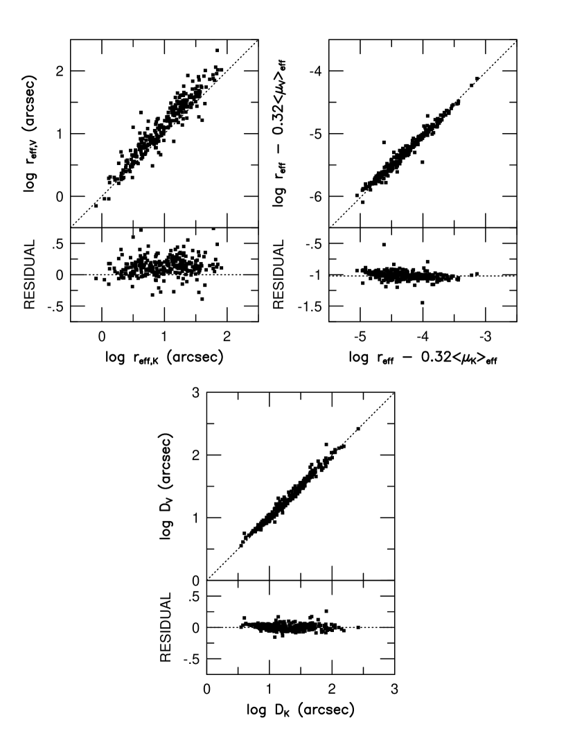
Figure 1: Comparison between the estimates of the effective radius $r_{\rm eff}$ and diameter $D$ (i.e., $D_{V}$ for the $V$–band, $D_{K}$ for the $K$–band). The quantity $r_{\rm eff}$ differs between the optical and near–infrared. The median offset for the comparison with the data of Lucey et al. (1991b, 1997) is $\log r_{\rm eff,V}-\log r_{\rm eff,K}=0.08$ dex. This systematic variation is consistent with a color gradient of $\Delta(\mu_{V}-\mu_{K})/\Delta\log r_{\rm eff}=-0.18$ mag dex^-1, which is a good match to the observed color gradients in $(B-R)$ and $(U-R)$ if their origin is in radial variations in [Fe/H] (see text).

The comparison between radii and diameters, as measured independently in the optical and near–infrared, are plotted in Figure 1. There is a clear, systematic difference between $\log r_{\rm eff,K}$ and $\log r_{\rm eff,opt}$, in the sense that the infrared effective radii are smaller than the optical ones. The $r_{\rm eff,opt}$ from the literature were not corrected for wavelength effects (as they should be due to the presence of color gradients), hence it is necessary to use subsamples for individual filters to make a meaningful comparison between optical and near–infrared effective radii. For example, comparing $r_{\rm eff,V}$ from Lucey et al. (1991b, 1997) with $r_{\rm eff,K}$ shows a median offset of $\log r_{\rm eff,V}-\log r_{\rm eff,K}=+0.08$ dex ($N=94$). This can be understood most simply as a change in scale length between the optical and near–infrared. Using the formalism of Sparks & Jørgensen (1993), the change in scale length implied by a color gradient is $\Delta s=\Delta r_{\rm eff}/r_{\rm eff}=0.18$, which is converted into an isophotal color gradient of $\Delta(\mu_{V}-\mu_{K})=\beta\Delta\log r$ with $\beta\sim\Delta s=-0.18$ mag arcsec^-2 dex^-1. This is similar to $\beta=-0.16$ mag arcsec^-2 dex^-1 found by Peletier et al. (1990b), albeit for a small sample (12 galaxies) with a small FOV detector. If the color gradient were due to a metallicity gradient, a simple change from [Fe/H]$=0$ to $-0.25$ dex would produce a change in color of $\Delta(V-K)=0.38$ mag, $\Delta(B-V)=0.07$ mag, $\Delta(U-R)=0.25$ mag, $\Delta(B-R)=0.11$ mag (Worthey (1994)). Thus, a metallicity gradient of $\Delta$ [Fe/H] $/\Delta\log r=-0.12$ would be consistent with the observed $\log r_{\rm eff,opt}-\log r_{\rm eff,K}=+0.08$ dex and the observed optical color gradients from the literature (Sandage & Visvanathan (1978); Franx, Illingworth, & Heckman (1989); Peletier et al. 1990a ; Jørgensen, Franx, & Kjærgaard 1995a ). If the trend of $(\log r_{\rm eff,opt}-\log r_{\rm eff,K})$ with $\log r_{\rm eff,K}$ is real, then this would also be consistent with the size of the color gradients correlating with galaxy size and hence luminosity.

It is also apparent that there is no systematic offset between $\log D_{V}$ and $\log D_{K}$, which is due to the good match between the assumed mean galaxy colors of $(V-K)=3.2$ mag used in the definition of $D_{K}$ and the true mean galaxy color. The rms of this difference is $0.048$ dex, which is significantly larger than the uncertainties in both measurements added in quadrature. Part of this effect is due to the change in the slope of the FP between the optical and near–infrared which causes a correlation of $\log D_{K}-\log D_{V}$ with $\log\sigma_{0}$. This effect will be discussed in §4.

There is a systematic offset of the quantity $(\log r_{\rm eff,K}-0.32\langle\mu_{K}\rangle_{\rm eff})-(\log r_{\rm eff,V}-0.32\langle\mu_{V}\rangle_{\rm eff})$ in Figure 1 which is primarily due to the mean color in $(V-K)$, but some of this effect is also due to the correlation with $\sigma_{0}$ due to the change in the slope of the FP between the optical and near–infrared.

4 The Difference in Slope Between the Optical and Near–Infrared FP

4.1 The Traditional Method to Measure the Change in Slope of the FP

The near–infrared FP has been shown in Pahre et al. (1998) to be represented by the scaling relation $r_{\rm eff}\propto\sigma_{0}^{1.53\pm 0.08}\langle\Sigma_{K}\rangle_{\rm eff}^{-0.79\pm 0.03}$. This relation shows a significant deviation from the optical forms of the FP: $r_{\rm eff}\propto\sigma_{0}^{1.24\pm 0.07}\langle\Sigma\rangle_{\rm eff}^{-0.82\pm 0.02}$ (Jørgensen, Franx, & Kjærgaard (1996)) and $r_{\rm eff}\propto\sigma_{0}^{1.38\pm 0.04}\langle\Sigma\rangle_{\rm eff}^{-0.82\pm 0.03}$ (Hudson et al. (1997)) in the $R$–band; or $r_{\rm eff}\propto\sigma_{0}^{1.13}\langle\Sigma\rangle_{\rm eff}^{-0.79}$ in the $V$–band (Guzmán, Lucey, & Bower (1993)). A simple conclusion can be drawn from these data: the slope of the FP increases with wavelength. While the trend appears clear in all these comparisons, the statistical significance of any one comparison is not overwhelming. For example, the change in slope from $r$–band to $K$–band is $+0.29\pm 0.11$, which is at the $<3\,\sigma$ confidence level (CL).

4.2 The New, Distance–Independent Method to Measure the Change in Slope of the FP

A more direct comparison will be made in this section between the optical and near–infrared FP relations by explicitly fitting the difference in slope for only those galaxies in common between a given optical survey and the near–infrared survey using the same central velocity dispersions for both. This will provide reasonable estimates of both the change in slope and its uncertainty.

The method used here takes advantage of the observation that the quantity $(\log r_{\rm eff}-b\langle\mu\rangle_{\rm eff})$ in the FP has a value of $b\sim 0.32$ that is independent of the wavelength studied or fitting method adopted. Note, for example, that $b=0.326\pm 0.011$ for the $R_{\rm C}$–band (Hudson et al. (1997)), $b=0.328\pm 0.008$ for the $r$–band (Jørgensen, Franx, & Kjærgaard (1996)), $b=0.320\pm 0.012$ for the $I_{\rm C}$–band (Scodeggio, Giovanelli, & Haynes (1997)), and $b=0.314\pm 0.011$ for the $K$–band (Pahre, Djorgovski, & de Carvalho (1998)). This agreement occurs despite the different fitting methods employed in each study. By assuming $b\equiv 0.32$, the optical and near–infrared forms of the FP reduce to

$$\begin{array}[]{rcl}\log r_{\rm eff,K}({\rm arcsec})&=&\,\,a_{K}\log\sigma_{0}+0.32\langle\mu_{K}\rangle_{\rm eff}+c_{i,K}\\ \log r_{\rm eff,opt}({\rm arcsec})&=&\,\,a_{\rm opt}\log\sigma_{0}+0.32\langle\mu_{\rm opt}\rangle_{\rm eff}+c_{i,{\rm opt}}\end{array}$$ (1)

Taking the difference of these equations produces

$$(\log r_{\rm eff,K}-0.32\langle\mu_{K}\rangle_{\rm eff})-(\log r_{\rm eff,opt}-0.32\langle\mu_{\rm opt}\rangle_{\rm eff})=\Delta a\times\log\sigma_{0}+c_{K,{\rm opt}}$$ (2)

where $\Delta a=a_{K}-a_{\rm opt}$ is the difference in FP slope between the near–infrared and optical, and the constants have been combined into $c_{K,{\rm opt}}$. There is no distance dependence on either the left–hand or right–hand sides of Equation 2, assuming that seeing corrections have been applied to $r_{\rm eff}$ and $\langle\mu\rangle_{\rm eff}$, and aperture corrections to $\sigma_{0}$. Therefore, all galaxies, both in clusters and the field, can be studied. When the optical FP is subtracted from the near–infrared FP, as has been done for Equation 2, then the left–hand side of the equation is related to the mean color offset between the two bandpasses—albeit corrected for a small, but systematic, reduction in effective radius from the optical to the near–infrared bandpasses.

Some literature sources measure a $D_{n}$ parameter instead of $r_{\rm eff}$ and $\langle\mu\rangle_{\rm eff}$, hence an equivalent equation for the change in slope of the $D_{n}$–$\sigma_{0}$ relation is

$$\log D_{K}-\log D_{\rm opt}=\Delta a\times\log\sigma_{0}+c_{K,{\rm opt}}.$$ (3)

All of the galaxies in the $K$–band sample with companion optical measurements of $r_{\rm eff}$ and $\langle\mu\rangle_{\rm eff}$ or $D_{n}$ were fit to Equations 2 or 3, respectively. The sum of the absolute value of the residuals was minimized in a direction orthogonal to the relation using the program GAUSSFIT (Jefferys et al. (1987)), and the uncertainties on $a$ and $c_{K,{\rm opt}}$ were determined from bootstrap resampling of the data. This combined sample used mean colors to convert data in the $B$, $r$, $R_{\rm C}$, or $I_{\rm C}$ bands into the $V$–band, with the exception of the Faber et al. (1989) data set, for which the observed $(B-V)_{0}$ were used. The problem with using mean colors is that no account is made for the color–magnitude relation between the observed and $V$ bandpasses, hence the slope of the FP does not change by construction. For this reason, separate comparisons are made for each literature source for those galaxies in common, but keeping the data in the original bandpass. All of these fits are listed in Table 1. Note that the catalogs prepared for the purpose of this comparison have been put onto a common extinction scale as described by Pahre (1998b). Several outlier data points were excluded from these fits: D45 in Klemola 44, PER199 in Perseus, and D27 in Coma from the comparison with Faber et al. (1989); E160G23 and NGC 4841A/B in Coma from the comparison with Scodeggio et al. (1997); and NGC 6482 from all comparisons.

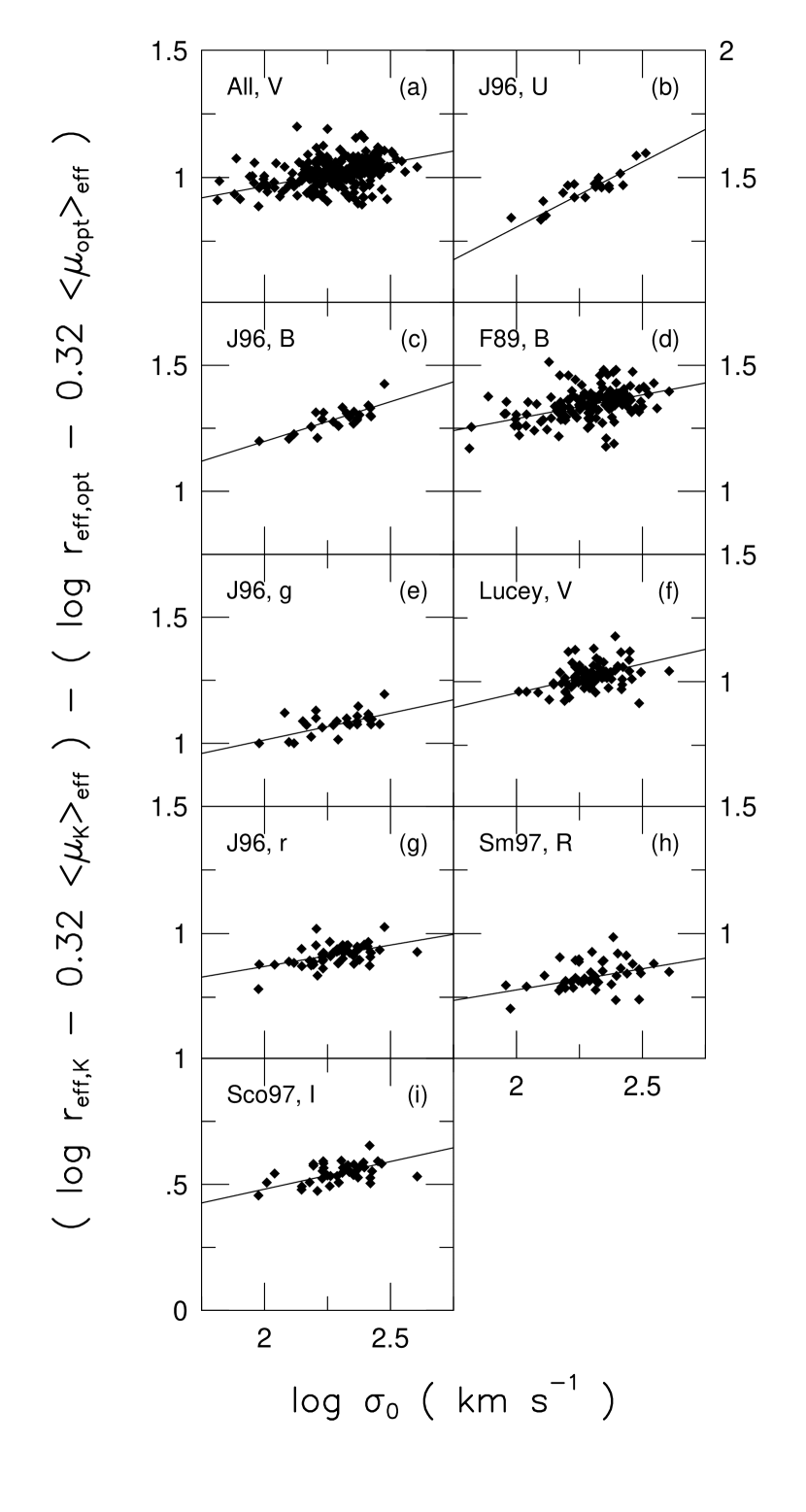
Figure 2: Comparison of the slope of the optical and near–infrared FP relations. Plotted as the vertical axis is the difference in $\log r_{\rm eff}-0.32\langle\mu\rangle_{\rm eff}$ in the sense of $K$–band minus optical, while velocity dispersion is the horizontal axis. If the optical and near–infrared FP relations had identical slopes, then the points would lie on a horizontal line. The positive value of the linear regression in each case signifies a steepening of the FP as the wavelength moves from the optical to the near–infrared. The slopes and intercepts of these comparisons are listed in Table 1. The literature comparisons are: Faber et al. (1989; F89); Lucey & Carter (1988), Lucey et al. (1991a,b), and Lucey et al. (1997); Jørgensen et al. (1996; J96); Smith et al. (1997; Sm97); and Scodeggio et al. (1997; Sco97).

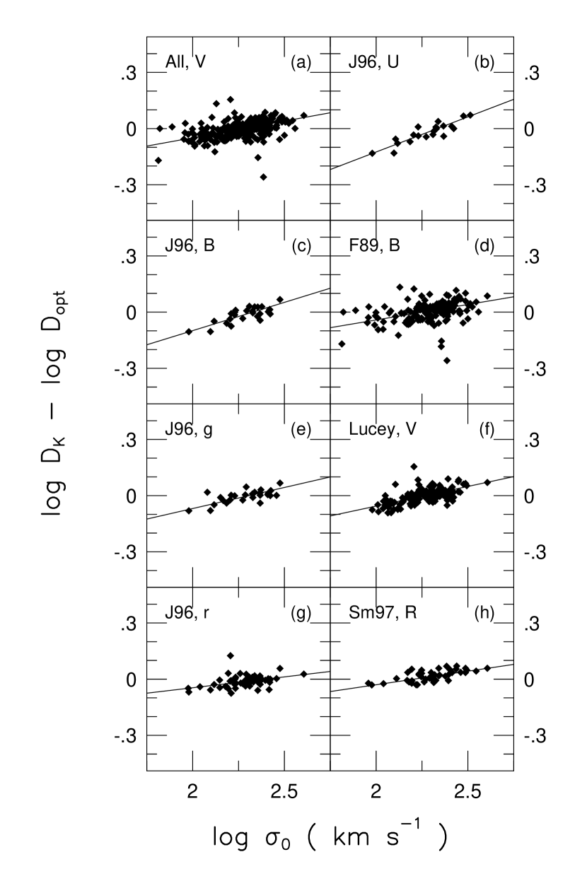
Figure 3: Comparison of the slope of the optical and near–infrared $D_{n}$–$\sigma_{0}$ relations. Plotted as the vertical axis is the difference in $\log D_{K}-\log D_{\rm opt}$, while velocity dispersion is the horizontal axis. If the optical and near–infrared FP relations had identical slopes, then the points would lie on a horizontal line. The positive value of the linear regression in each case signifies a steepening of the FP as the wavelength moves from the optical to the near–infrared. The literature comparisons are the same as in Figure 2.

The fits for each of the subsamples are plotted in Figures 2 and 3 for the comparisons of $\log r_{\rm eff}-0.32\langle\mu\rangle_{\rm eff}$ and $D_{n}$, respectively. If the optical and near–infrared FP relations had the same slope, then all points would lie on a horizontal line in these figures; this is clearly not the case. The statistical significance of each regression for the comparison of $(\log r_{\rm eff}-0.32\langle\mu\rangle_{\rm eff})$ is at the 2–6 $\sigma$ confidence level (CL), while the significance for the $(\log D_{K}-\log D_{\rm opt})$ comparison is at the 3–10 $\sigma$ CL. As a demonstration of how the method adopted here is superior to the alternate method of fitting the optical and near–infrared FP relations independently and then comparing their slopes, notice that the $0.06$ dex uncertainty in Table 1 for the Jørgensen et al. (1996) $r$–band subsample is nearly a factor of two smaller than the $0.11$ dex uncertainty derived when the independently fitted slopes were compared in §4.1, despite the fact that one–fourth the number of galaxies were used in this newer method. The difference is most likely due to several factors: an identical sample of galaxies is studied simultaneously in both the optical and near–infrared; the velocity dispersion term used is identical for both FP relations; there is no assumption about the distance to a given galaxy or its cluster; and the uncertainties in the velocity dispersion are not applied twice in the estimation of uncertainties.

All of the optical to near–infrared comparisons of $(\log r_{\rm eff}-0.32\langle\mu\rangle_{\rm eff})$, with the exception of the $U$–band comparison with Jørgensen et al. (1995a), are statistically indistinguishable. The uncertainties, however, are large enough that small but real trends with wavelength in the optical are not excluded. While the $D_{n}$–$\sigma_{0}$ relations show no statistical difference between the $B$ and $V$ bandpasses, there is a change in the slope between the optical to near–infrared data (significant at the 2–3 $\sigma$ CL) from the $V$ to the $R$ (or $r$) bandpasses, or from the $U$ to any other bandpass. The reason that the $B$ band does not match this trend, or that the $(\log r_{\rm eff}-0.32\langle\mu\rangle_{\rm eff})$ comparison did not show the effect, is that these other comparisons have substantially larger observational measurement uncertainties. The $D_{n}$ parameter can be measured 10–50% more reliably than $(\log r_{\rm eff}-0.32\langle\mu\rangle_{\rm eff})$, whether in the optical (Jørgensen, Franx, & Kjærgaard (1996); Smith et al. (1997); Lucey et al. (1997)) or near–infrared (Pahre 1998b ).

4.3 Possible Environmental Effects on the FP

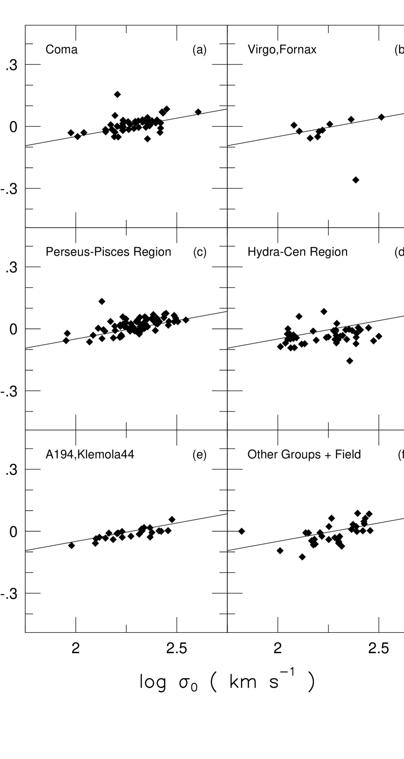
Figure 4: Comparison of the difference in slope and intercept of the $D_{V}$–$\sigma_{0}$ and $D_{K}$–$\sigma_{0}$ relations in various regions and density environments. The same straight line fit to the entire sample is displayed in each panel to ease comparison. Note how there is little or no difference between the slope or intercept in any panel and the mean relation. The largest possible offset is in the Hydra–Centaurus region, but this effect is smaller and of opposite sign when compared to the effect found by Guzmán (1995). The large difference between Guzmán (1995) and the present work is fully explained by different assumptions of Galactic extinction in the Hydra–Centaurus region; the formal uncertainty on the IRAS 100$\mu$m to $A_{B}$ extinction conversion adopted here is consistent with there being no offset between the mean relation and the Hydra–Centaurus galaxy subsample. This figure provides evidence that there are no significant environmental effects on the $D_{n}$–$\sigma_{0}$ relation.

A significant offset in the relationship between $(\log D_{K}-\log D_{V})$ and $\log\sigma_{0}$, as measured separately in the Coma cluster and the Hydra–Centaurus Region, was identified by by Guzmán (1995). If this were the case, it would suggest that there are significant environmental effects on the elliptical galaxy correlations, thereby preventing their utility as accurate distance indicators. The present paper includes larger samples of galaxies both in Coma and Hydra–Centaurus, as well as other rich clusters and low density environments, hence this effect can be re–analyzed. The data were broken down into six regions of the sky or similar density environments, compared to the overall solution (as listed in Table 1), and are displayed in Figure 4.

Guzmán (1995) found that $(\log D_{K}-\log D_{V})$ at a given $\log\sigma_{0}$ was $\sim 0.05$ dex larger in Hydra–Centaurus region than in Coma, but panel (d) of Figure 4 shows that it is $<0.03$ dex smaller. Most of the difference between the results of Guzmán and the present work can be explained by different assumptions of Galactic extinction: he apparently used Burstein & Heiles (1982) maps (which are based on galaxy number counts and neutral gas emission) as the estimator of $A_{B}$, while this work uses the 100$\mu$m emission (as measured by IRAS) as the estimator of $A_{B}$. While the two estimates agree fairly well in a global sense, they disagree by 0.1–0.2 mag in Hydra–Centaurus, in the sense that Burstein & Heiles (1982) underestimates $A_{B}$. Nonetheless, the formal error on $A_{B}$ due to the uncertainties of the IRAS conversion in Laureijs, Helou, & Clark (1994), are sufficient to bring all the galaxies in this region into agreement with the global relation between $(\log D_{K}-\log D_{V})$ and $\log\sigma_{0}$. Furthermore, the somewhat larger scatter of the galaxy properties found in this region, compared to the cluster subsamples in the other panels, also argues for significant, patchy dust extinction. It is interesting to note that by increasing $A_{B}$ in Hydra–Centaurus, the distance estimations of Lynden–Bell et al. (1988) would place these galaxies closer to us, thereby strengthening the statistical evidence for a Great Attractor causing bulk motions of the galaxies in this region.

Inspection of Figure 4 leads to the conclusion that there is no evidence that either the slope or intercept of the elliptical galaxy correlations are dependent on environment. For example, the difference in intercepts between the field and group sample ($N=32$) and all other galaxies ($N=213$; both using a $\pm 0.15$ dex clip to exclude outliers) in Figure 4 is only $0.010\pm 0.009$ dex, which corresponds to a difference of $0.03\pm 0.03$ mag in $(V-K)$ between the two sub-samples (in the sense that the field galaxies are marginally bluer). Using the Bruzual & Charlot (1996) models, this offset in $(V-K)$ color constrains the difference in mean age between field and cluster early–type galaxies to be $\leq 0.045$ dex. The extinction correction $E(V-K)=0.65A_{B}$, so uncertainties in $A_{B}$ of $\geq 0.05$ mag (which corresponds to the $\Delta(V-K)=0.03$ mag effect on the intercept) are obtained for $A_{B}\geq 0.3$ mag in the Laureijs et al. (1994) extinction estimates. Extinction estimates for the Hydra–Centaurus region, Perseus, and Pegasus exceed this value, while high latitude clusters such as Coma, Abell 2199, Klemola 44, and Fornax have little or no extinction; the field and group sample shows a wide range in extinction $0.01\geq A_{B}\geq 0.84$ mag (Pahre 1998b ). Uncertainties in foreground Galactic extinction therefore appear to be the dominant source of uncertainty contributing to any possible differences between field and cluster early–type galaxies measured using this method. The difference in FP intercept and scatter between galaxies in clusters and the general field found by de Carvalho & Djorgovski (1992) would be naturally explained by errors in estimating dust extinction (which also affects the present paper) or estimating distances (which does not affect the present paper), and not by any intrinsic differences in the stellar populations among elliptical galaxies that correlates with their environment. Difficulties in estimating Galactic dust extinction therefore appear to be the limiting factor for optical distance scale work using the elliptical galaxy correlations. The sample used here is also small (only $\sim 30$ galaxies in loose groups and the general field), hence these results naturally require confirmation with larger galaxy samples.

While stellar populations variations with environment appear to be excluded by the results in Figure 4, the effects due to variations in homology breaking or dark matter content with environment would cancel out in this figure and analysis. Hence, environmental variations that appear as a wavelength independent property, such as homology breaking or systematic variations in dark matter content, are not constrained by this analysis. A test for these effects could entail comparing the slope of the FP, as measured separately at $V$ and $K$ (as in §4.1), between clusters and the field. Unfortunately, such a test will suffer from systematic errors due to distance which were eliminated in the approach advocated in §4.2. The use of an accurate distant indicator (such as surface brightness fluctuations; Tonry et al. (1997)) could circumvent this problem; such an analysis will be reserved for a future contribution.

In summary, while there appear to be no variations in the intercept of the FP with environment due to stellar populations effects, this result is uncertain at the level of the correction for Galactic extinction and subject to the assumption that the slope of the FP is not varying with environment. The issue of whether there exists variations in homology breaking or dark matter content with environment is left open.

5 Comparing the Fundamental Plane Among Various Optical Bandpasses

When comparing the optical and near–infrared FP in §4, there were hints that the differences might be larger for the $U$–band than for, say, the $R_{\rm C}$–band. Small changes of the slope of the FP between $U$ and $r$, for example, were reported by Jørgensen et al. (1996) and Djorgovski & Santiago (1993) in the sense that the $U$–band FP has the shallowest slope. Although the differences determined in this manner were of small significance, it should be possible to improve the significance by removing the distance assumptions and using the method described above. Catalogs of optical global photometric parameters and velocity dispersions were compiled from the literature in the same manner as for the near–infrared catalogs (see Pahre 1998b ). An additional catalog consisting of $(U-B)$, $(B-V)$, $(V-R_{\rm C})$, and $(V-I_{\rm C})$ colors and velocity dispersion was constructed from Prugniel & Simien (1996) without modification. Since Prugniel & Simien do not measure $r_{\rm eff}$ and $\langle\mu\rangle_{\rm eff}$ independently for each of the five bandpasses, the differences in $\log r_{\rm eff}-0.32\langle\mu\rangle_{\rm eff}$ were taken to be $0.32$ multiplied by the color. This approach is only partially correct since it does not account for the presence of color gradients, but the systematic errors resulting from this simplification are small.

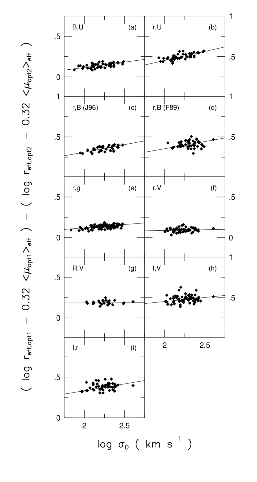
Figure 5: Comparison of the slope of the FP relations among various optical bandpasses from $U$ to $I_{\rm C}$. In each panel, the vertical axis is the difference in $r_{\rm eff}-0.32\langle\mu\rangle_{\rm eff}$ measured in each of the pair of bandpasses; the bandpasses are identified in the upper–left corner of each panel, and the difference is in the sense of the first bandpass minus the second. The FP slope is steeper in redder bandpasses as is evidenced by the positive correlation in nearly every panel. Literature sources and regressions are taken from Table 9.

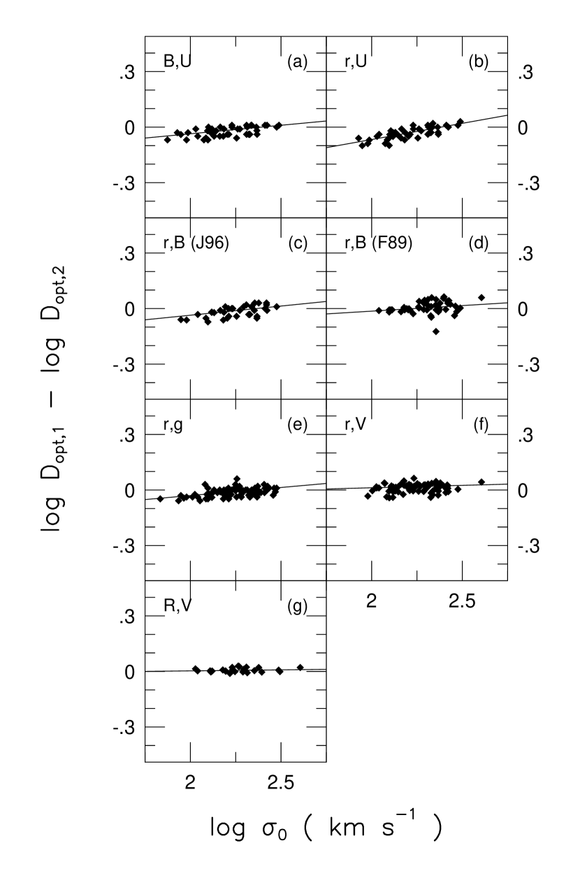
Figure 6: Comparison of the slope of the $D_{n}$–$\sigma_{0}$ relation among various optical bandpasses from $U$ to $I_{\rm C}$. In each panel, the vertical axis is the difference in $\log D_{n}$ measured in each of the pair of bandpasses; the bandpasses are identified in the upper–left corner of each panel, and the difference is in the sense of the first bandpass minus the second. The slope of the $D_{n}$–$\sigma_{0}$ relation is steeper in redder bandpasses as is evidenced by the positive correlation in nearly every panel. Literature sources and regressions are taken from Table 9.

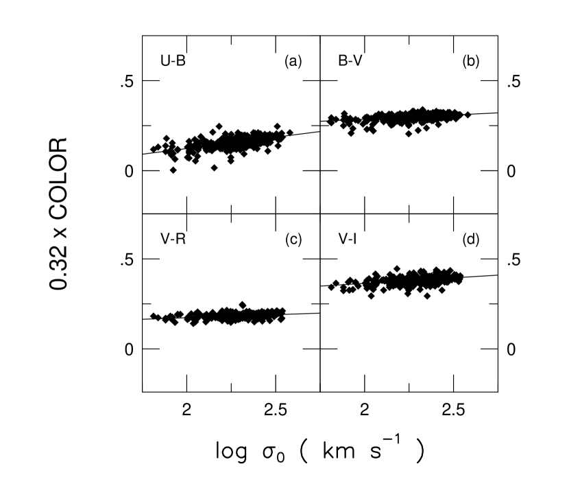
Figure 7: Approximate comparison of the slope of the FP relations between various optical bandpasses using the color information from Prugniel & Simien (1996). Since those authors did not measure $r_{\rm eff}$ and $\langle\mu\rangle_{\rm eff}$ independently for each bandpass, the quantity 0.32 times the color was substituted for the difference in $r_{\rm eff}-0.32\langle\mu\rangle_{\rm eff}$ between each pair of bandpasses. This approach is reasonably similar to Figure 5, although it does not fully account for the effects of color gradients on the slope of the FP. Regressions are taken from Table 9. Notice that all panels show a regression with positive slope, once again indicating that the slope of the FP steepens with wavelength.

All comparisons demonstrate that the redder bandpass has a steeper slope for the FP as evidenced by a positive $\Delta a$, although in several cases $\Delta a$ is statistically indistinguishable from zero. The comparisons derived from surface photometry are displayed in Figures 5 and 6, while those derived from color information alone (i.e., Prugniel & Simien (1996)) are displayed in Figure 7.

In several comparisons where the two bandpasses differ only slightly in wavelength—such as between the $r$–band and $V$–band—there is no significant variation of the slope of the FP. In most cases, however, there is a statistically significant 3–13 $\sigma$ CL positive regression, and in no case is there a negative regression, in the analysis listed in Table 9.

6 General Constraints from the Elliptical Galaxy Scaling Relations

The preceding section, and a number of earlier papers, describe a series of global properties of early–type galaxies that are elucidated from the exact forms of the scaling relations in various bandpasses. These can be summarized as:

1. Early–type galaxies are well–described by a Fundamental Plane corresponding to the scaling relation $r_{\rm eff}\propto\sigma_{0}^{1.53\pm 0.08}\langle\Sigma_{K}\rangle_{\rm eff}^{-0.79\pm 0.03}$ (Pahre, Djorgovski, & de Carvalho (1998)).

2. As has been shown in §4, the slope of the FP (the exponent for the $\sigma_{0}$ term) steepens significantly between the optical and near–infrared. As shown in §5, the slope of the FP steepens with wavelength even among the optical bandpasses.

3. The slope of the FP at all wavelengths is inconsistent with the relation $r_{\rm eff}\propto\sigma_{0}^{2}\langle\Sigma\rangle_{\rm eff}^{-1}$ which is expected from the virial theorem under the assumptions of constant mass–to–light ratio and homology within the family of elliptical galaxies.

4. The FP and Mg₂–$\sigma_{0}$ relations may be thin, but they have significant, resolved intrinsic scatter which cannot be explained by the observational uncertainties and does not have a clear correlation with any particular indicator of metallicity or age (Jørgensen, Franx, & Kjærgaard (1996); Pahre, Djorgovski, & de Carvalho (1998)).

5. The effective radius of early–type galaxies was shown in §3 to be systematically smaller at longer wavelengths, which is basically equivalent to the existence (and size) of color gradients in these galaxies if they result from metallicity gradients (Peletier (1993)).

There are several other relevant properties of early–type galaxies that can be added to the above list but were not directly shown in this paper:

1. The velocity dispersion measured in an aperture decreases with the increasing size of this aperture according to a power law; the exponent of this power law appears to show a correlation with the luminosity or size of the galaxy (Jørgensen, Franx, & Kjærgaard 1995b ; Busarello et al. (1997)).

2. The ratio of magnesium to iron appears to be over-produced in early–type galaxies relative to the solar value (Worthey, González, & Faber (1992)), albeit with a significant spread in [Mg/Fe], implying the importance of type II supernovae chemical enrichment and rapid massive star formation in the galaxy formation process, particularly for the most luminous elliptical galaxies.

3. The correlation of Mg₂ with $\sigma_{0}$ implies a connection between the chemical enrichment of a galaxy and the depth of its potential well.

4. Optical and near–infrared color gradients in elliptical galaxies imply isophotal populations gradients of the order $0.16$ to $0.30$ dex in [Fe/H] (or 1.5 times this in $\log$ age) per decade of radius (Franx et al. 1989; Peletier et al. 1990a,b; Peletier (1993)).

5. There is no known correlation between the size of the measured color gradient and the luminosity of the host galaxy (Peletier et al. 1990a), although some of the smallest galaxies show no gradients altogether.

Any viable model to explain the global properties of early–type galaxies must be able to account for all of these effects.

7 A Self–Consistent Model for the Underlying Physical Parameters Which Produce the FP Correlations

In this section, a series of models will be constructed and explored in order to determine if all the observational constraints in §6 can be explained in a fully consistent manner.

7.1 Modeling the Changes in the Slope of the FP Between Bandpasses

The effects on broadband color of the change in slope of the FP with wavelength can be expressed in a simple manner. Starting with the definition of total magnitude for a de Vaucouleurs profile,

$$m_{\rm tot}=-5\log r_{\rm eff}+\langle\mu\rangle_{\rm eff}-2.5\log 2\pi$$ (4)

and the definition of the change in slope $\Delta a_{j,i}$ of the FP from bandpass $j$ to bandpass $i$ (Equation 2), the change in the global color $\Delta C_{i,j}$ between bandpass $i$ and $j$ is then

$$\begin{array}[]{rcl}\Delta C_{i,j}&=&3.125\left[\left(\log r_{\rm eff,j}-0.32\langle\mu_{j}\rangle_{\rm eff}\right)-\left(\log r_{\rm eff,i}-0.32\langle\mu_{i}\rangle_{\rm eff}\right)\right]\\ &&-1.875\left(\log r_{\rm eff,i}-\log r_{\rm eff,j}\right)\\ &=&3.125\Delta a_{j,i}\Delta\log\sigma_{0}-1.875\Delta r_{\rm eff,i,j}\end{array}$$ (5)

where $\Delta r_{\rm eff,i,j}$ is the change of $\log r_{\rm eff}$ from bandpass $i$ to bandpass $j$, and $\Delta\log\sigma_{0}\sim 0.6$ dex is the change in $\log\sigma_{0}$ from one end of the FP to the other (a range within which $>90$% of the galaxies lie). The two terms on the right–hand side in Equation 5 show the effects of the change in slope of the FP and the presence of color gradients, respectively.

In multi–color studies of isophotal color gradients in elliptical galaxies, Peletier et al. (1990a,b) and Franx et al. (1989) found consistent results if the underlying cause were metallicity gradients of $-0.20$, $-0.16$, and $-0.3$ dex, respectively. A simple stellar populations model can then be used to convert these estimates into any broadband isophotal color gradient $\beta$ between $U$ and $K$. The conversion from isophotal color gradient to $\Delta\log r_{\rm eff}$ is accomplished using Equation 21 of Sparks & Jørgensen, such that $\Delta\log r_{\rm eff}=\beta/(2.3\times 1.20)$. Hence, only one parameter to represent the global mean metallicity gradient is introduced into the sets of equations described by Equation 5 for the 22 observed $\Delta a_{j,i}$ from Tables 1 and 9.

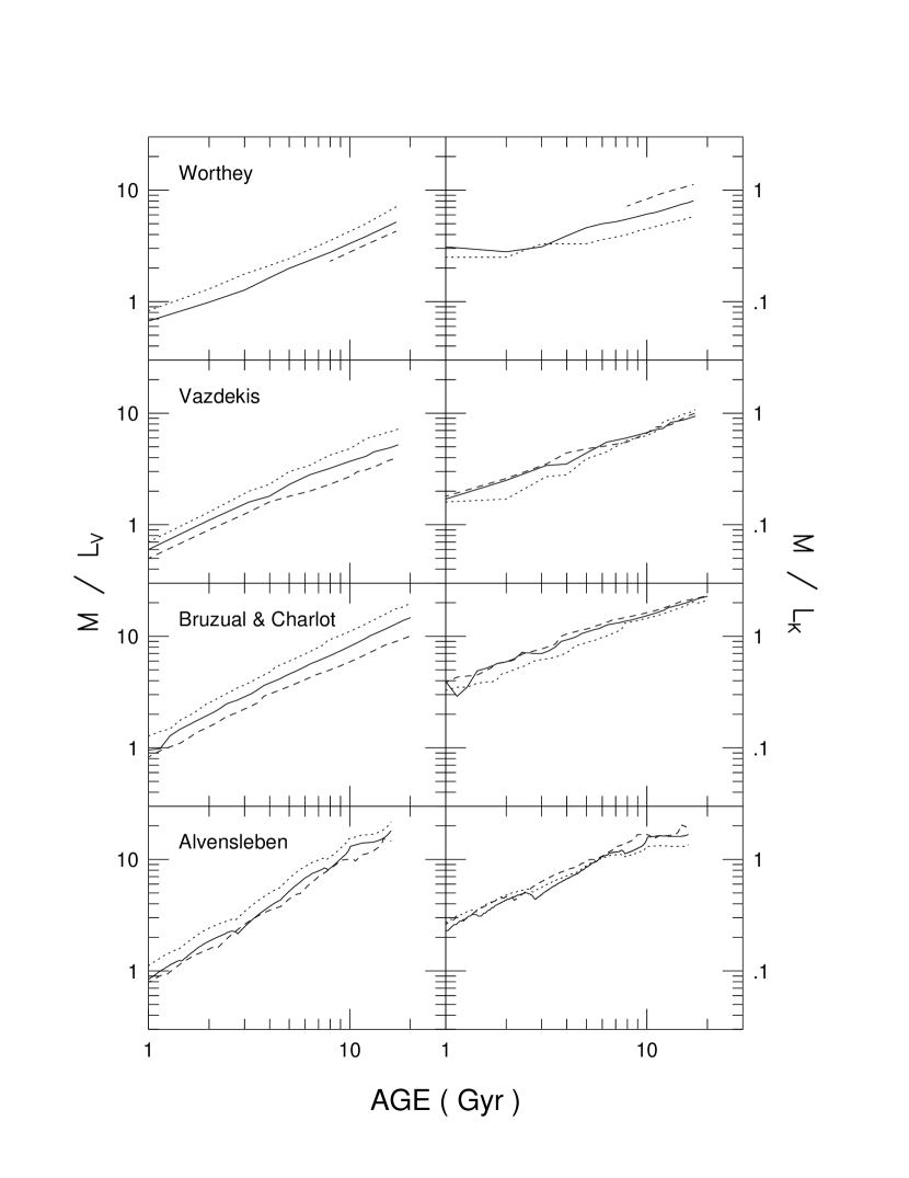
Figure 8: Comparison of $M/L_{V}$ (left) and $M/L_{K}$ (right) for four different stellar populations models from Worthey (1994), Vazdekis et al. (1996), Bruzual & Charlot (1996, in preparation; as provided in Leitherer et al. (1996)), and Fritze-V. Alvensleben & Burkert (1995). Iron abundances of [Fe/H]$=-0.4$ (dashed line), $0.0$ (solid line), and $+0.4$ dex (dotted line) are shown, except for the Fritze-v. Alvensleben & Burkert (1995) models which have the $+0.3$ dex model substituted for $+0.4$ dex. All models show similar variations in $M/L_{V}$ with both time and abundance, but not $M/L_{K}$. In particular, the Worthey (1994) models show a dependence of $M/L_{K}$ on [Fe/H]—such that metal–rich systems have small $M/L_{K}$—while the Vazdekis et al. and Bruzual & Charlot models have $M/L_{K}$ independent of metal abundance.

There is a significant difference in $M/L$ even among the most sophisticated of simple stellar populations models (Charlot, Worthey, & Bressan (1996)). Nonetheless, use of such models in a differential sense shows far less variation among the models. An example of this is given in Figure 8, where the mass–to–light ratio in the $V$–band and $K$–band is compared for four such models. For large ages $t\geq 10$ Gyr, both the Vazdekis et al. (1996) and the Bruzual & Charlot (1996, as provided in Leitherer et al. (1996)) models show similar behavior with $M/L_{K}$ independent of [Fe/H], while the Worthey (1994) models have $M/L_{K}$ inversely dependent on [Fe/H] and the Fritze-V. Alvensleben & Burkert (1995) models are inconclusive. In fact, Charlot, Worthey, & Bressan (1996) showed in detail how three models differ strongly in their near–infrared properties. From the inspection of the near–infrared portion of Figure 8, we have chosen only to make detailed comparisons with the Vazdekis et al. and Bruzual & Charlot models.

An additional question could be posed based on Figure 8: given that there are significant spreads in $M/L$ between the four models at any wavelength, are the changes in $M/L$ (by varying the age and/or metal abundance) more consistent between the models? This was addressed by Charlot et al. (1996) who showed that the variations among three models was of order $\delta(B-V)/\delta t\sim 0.004$ mag Gyr^-1, $\delta(V-K)/\delta t\sim 0.015$ mag Gyr^-1, and $\delta(M/L_{V})/\delta t\sim 0.1$ M_⊙ L${}_{\odot}^{-1}$ Gyr^-1 at $t\sim 10$ Gyr. Hence a given model can be used to measure differential age or metallicity effects for an old stellar population while not providing an accurate absolute measure of either quantity.

The variations in magnitude as a function of changing [Fe/H] from $-0.4$ dex to $+0.4$ dex at $t=11$ Gyr, and separately as a function of changing age from 2 to 17 Gyr (at intervals of 1 Gyr) at [Fe/H] $=0$ dex, were calculated using the Bruzual & Charlot models for the $UBVR_{\rm C}I_{\rm C}K$ bandpasses. The same calculations were made for the Vazdekis et al. (1996) models. For the modeling below, the Gunn $r$–band will be assumed identical (for differential effects) to the Cousins $R_{\rm C}$–band, the Gunn $g$–band will be assumed identical to the $V$–band, and the $K_{s}$–band assumed identical to the $K$–band. These calculations are summarized in Table 3.

7.2 Additional Equations of Constraint

The fit to the Mg₂–$\sigma_{0}$ relation (Pahre, Djorgovski, & de Carvalho (1998)) provides an additional equation of constraint derived from the Bruzual & Charlot models (using the variations specified in Table 3), namely

$$0.173\pm 0.010=\left[0.174\Delta\log t+0.278\left(\Delta{\rm~{}[Fe/H]}+\left({\Delta{\rm~{}[Fe/H]}\over 1.2\times 1.6\Delta\log r}\right)\right)\right]\Delta\log\sigma_{0}$$ (6)

The factor of 1.2 in the denominator converts the isophotal gradients into linear changes in $r_{\rm eff}$ (from Equation 21 of Sparks & Jørgensen (1993)), while the factor of 1.6 converts this change in $r_{\rm eff}$ into an aperture populations gradient (Sparks & Jørgensen (1993), Equation 18). This latter point is essential to recognize since Mg₂ is typically measured in an aperture of fixed physical size—and has been corrected to a fixed physical size using the methodology of Jørgensen et al. (1995b).

In all cases, an isophotal populations gradient of $\beta=\Delta(\mu_{i}-\mu_{j})/\Delta\log r$ between bandpasses $i$ and $j$ is converted to an equivalent change in effective radius $\Delta r_{\rm eff,i,j}=\beta/(1.2\times 2.3)$, where the factor of 2.3 comes from converting the linear change in $r_{\rm eff}$ to logarithmic and the factor of 1.2 derives from Equation 21 of Sparks & Jørgensen (1993).

The slope of the FP in the $K$–band provides another equation of constraint, as its slope can be affected by age and deviations from homology, but virtually not by metallicity. From the fit to the Faber–Jackson (1976) relation in the $K$–band (Pahre, Djorgovski, & de Carvalho (1998)), $\Delta K_{\rm tot}=10.35\Delta\sigma_{0}$, from Table 3 $\Delta K_{\rm tot}({\rm mag})=+1.48\Delta\log t-0.16\Delta$[Fe/H] (dex), so the luminosity along the sequence varies as

$$\gamma={+1.48\Delta\log t-0.16\Delta{\rm~{}[Fe/H]~{}}({\rm dex})\over 10.35\Delta\log\sigma_{0}}$$ (7)

In this way the slope of the $K$–band FP (i.e., $a$ in $r_{\rm eff}\propto\sigma_{0}^{a}$; Pahre, Djorgovski, & de Carvalho (1998)) provides the equation of constraint

$$1.528\pm 0.083={1\over 1+d}\left({2\over 2\gamma+1}\right)$$ (8)

where a new model parameter $d$ was introduced to represent the deviations of the family of ellipticals from a homologous family in dynamical structures. In this notation, the mapping of velocity dispersions is $\log\sigma_{0}=(1+d)\log\sigma_{\rm eff}+{\rm~{}const.}$ to provide a systematic variation of $\log\sigma_{0}-\log\sigma_{\rm eff}$ along the elliptical galaxy sequence. Introduction of the model parameter $d$ also allows for an additional equation of constraint from the measurement of this mapping by Busarello et al. (1997), who found $d=0.28\pm 0.11$.

In summary, there are 22 equations of constraint represented by Equation 5 from the comparisons of the optical and near–infrared FP between pairs of bandpasses (where $\Delta a_{j,i}$ are provided in Tables 1 and 9), and one equation of constraint each from the Mg₂–$\sigma_{0}$ relation, the slope of the $K$–band FP relation, and the dynamical non-homology measurement. There are four free parameters: (1) the variation in age $\Delta\log t$ from one end of the FP to the other; (2) the variation in metallicity $\Delta$[Fe/H] along the same sequence; (3) the size of the stellar populations gradient (equal for all elliptical galaxies), expressed for convenience as a metallicity gradient, which produces a color gradient $\beta=\Delta(\mu_{i}-\mu_{j})/\Delta\log r$; and (4) the size of the dynamical non-homology contribution $d$ to the mapping from $\sigma_{0}$ to $\sigma_{\rm eff}$.

7.3 Solutions to the Physical Quantities in the Model for the Scaling Relations

The variance was minimized orthogonal to the fit and the uncertainties for each measurement were included in the construction of the Chi–squared statistic. The uncertainties for the four measurements of the change in slope of the optical FP for the Prugniel & Simien (1996) data set were intentionally doubled to account for the systematic effect that these data do not explicitly account for the effects of color gradients. The parameter $\Delta\log\sigma_{0}$ was set to $0.6$ dex to account for the range of velocity dispersion occupied by nearly all the elliptical galaxies; this number merely scales up the model parameters (except for $d$) without changing the significance of any parameter. The least–squares solution was for the following values of the model parameters

$$\begin{array}[]{rcl}\Delta\log t&=&+0.38\pm 0.20{\rm~{}dex}\\ \Delta{\rm~{}[Fe/H]}&=&+0.28\pm 0.14{\rm~{}dex}\\ {\Delta{\rm~{}[Fe/H]}\over\Delta\log r}&=&-0.26\pm 0.28{\rm~{}dex}\\ d&=&+0.17\pm 0.10\end{array}$$ (9)

The uncertainty estimates are taken from the covariance matrix. The reduced Chi–square for this fit is close to unity at $1.33$, suggesting that the combination of the model and the uncertainty estimates in each of the observables is a reasonable description of the properties of elliptical galaxies along their sequence.

The results given in Equation 9 for the first time describe the underlying physical origin of the elliptical galaxy scaling relations using a self–consistent model that accounts for population gradients, wavelength effects on the FP, systematic deviations from homology, and a metal line–strength indicator. The formal significance of the results in Equation 9, however, appear to suffer from low significance for any given parameter: $\Delta\log t$, $\Delta$[Fe/H], and $d$ are all only significant at the 2 $\sigma$ CL, while the populations gradient is virtually unconstrained and even consistent with zero. There is significant correlation between the model parameters which is the underlying cause of the reasonably large uncertainties on each parameter; the largest correlation coefficient is $-0.7$ between $d$ and $\Delta\log t$, which is not surprising since either parameter (or a combination of both) is essential for satisfying constraint from the slope of the near–infrared FP (Equation 8).

The inability to constrain the populations gradients should not be considered a problem, since this model is actually only an indirect way of measuring populations gradients in ellipticals; far better are direct measurements of Mg₂ line strength or color gradients. For all of the following fits, an additional equation of constraint will be included to represent the populations gradients: $\Delta{\rm~{}[Fe/H]}/\Delta\log r=-0.22\pm 0.01$ dex per decade of radius, as this is the mean of color and line–strength gradients from the literature in the analysis of Peletier (1993). The least–squares solution then becomes:

$$\begin{array}[]{rcl}\Delta\log t&=&+0.36\pm 0.15{\rm~{}dex}\\ \Delta{\rm~{}[Fe/H]}&=&+0.26\pm 0.11{\rm~{}dex}\\ {\Delta{\rm~{}[Fe/H]}\over\Delta\log r}&\equiv&-0.22\pm 0.01{\rm~{}dex}\\ d&=&+0.17\pm 0.09\end{array}$$ (10)

with $\chi^{2}/\nu=1.27$. When one or more parameters are set to zero, then the following series of solutions $(\Delta\log t,\Delta{\rm~{}[Fe/H]},d,\chi^{2}/\nu)$ are obtained:

$$\begin{array}[]{llll}\Delta\log t=+0.73&\Delta{\rm~{}[Fe/H]}=0&d=0&\chi^{2}/\nu=1.47\\ \Delta\log t=0&\Delta{\rm~{}[Fe/H]}=+0.50&d=0&\chi^{2}/\nu=3.20\\ \Delta\log t=0&\Delta{\rm~{}[Fe/H]}=0&d=0.30&\chi^{2}/\nu=41\\ \Delta\log t=+0.73&\Delta{\rm~{}[Fe/H]}=0&d=0.05&\chi^{2}/\nu=1.50\\ \Delta\log t=+0.58&\Delta{\rm~{}[Fe/H]}=+0.11&d=0&\chi^{2}/\nu=1.44\\ \Delta\log t=0&\Delta{\rm~{}[Fe/H]}=+0.51&d=0.32&\chi^{2}/\nu=1.52\end{array}$$ (11)

In all cases, there is a significant or substantial increase in $\chi^{2}/\nu$ by factors between 1.13 to 40, suggesting that the full set of model parameters is required to provide an accurate representation of the observables.

Using the Vazdekis et al. (1996) models instead of the Bruzual & Charlot (1996) models, but still keeping $\Delta{\rm~{}[Fe/H]}/\Delta\log r=-0.22\pm 0.01$ dex per decade of radius, produces the solution:

$$\begin{array}[]{rcl}\Delta\log t&=&+0.14\pm 0.07{\rm~{}dex}\\ \Delta{\rm~{}[Fe/H]}&=&+0.53\pm 0.05{\rm~{}dex}\\ {\Delta{\rm~{}[Fe/H]}\over\Delta\log r}&\equiv&-0.22\pm 0.01{\rm~{}dex}\\ d&=&+0.26\pm 0.07\end{array}$$ (12)

with $\chi^{2}/\nu=1.04$. Since the model uncertainties have not been included in the $\chi^{2}$ statistic, this reduction of 20% in $\chi^{2}/\nu$ for the Vazdekis et al. (1996) models over the Bruzual & Charlot (1996) models suggests that the former have a subtle improvement over the latter in their treatment of the photometric properties of old stellar populations. Contours of joint probability between pairs of the model parameters are plotted in Figure 9 for this solution.

If the differences in slope $\Delta a_{j,i}$ derived from the $D_{n}$–$\sigma_{0}$ relation are used instead of those from the quantity $\log r_{\rm eff}-0.32\langle\mu\rangle_{\rm eff}$, then the solution is

$$\begin{array}[]{rcl}\Delta\log t&=&+0.16\pm 0.09{\rm~{}dex}\\ \Delta{\rm~{}[Fe/H]}&=&+0.50\pm 0.05{\rm~{}dex}\\ {\Delta{\rm~{}[Fe/H]}\over\Delta\log r}&\equiv&-0.22\pm 0.01{\rm~{}dex}\\ d&=&+0.25\pm 0.11\end{array}$$ (13)

with a much poorer $\chi^{2}/\nu=3.04$. The difference in $\chi^{2}/\nu$ between this solution (using the differences in $D_{n}$) and the previous solution (using the differences in $\log r_{\rm eff}-0.32\langle\mu\rangle_{\rm eff}$) can be directly attributed to the significantly smaller uncertainties in the measurements of $\Delta a_{j,i}$ from the $D_{n}$–$\sigma_{0}$ relation in Tables 1 and 9. The same effect in $\chi^{2}/\nu$ is found when the Bruzual & Charlot models are used instead. We suspect that these small formal uncertainties arise due to a poor sensitivity of the $D_{n}$ parameter to the subtle effects of color gradients, despite the apparent homogeneity and repeatability in measuring this quantity. On the other hand, the difference could point to overall limitations of the model if these small uncertainties in $\Delta a_{j,i}$ are real.

7.4 The Relative Roles of Various Constraints on the Model Solution

Several remarks need to be made about the contribution of the various equations of constraint towards the self–consistent solutions described above. Broadband colors are notoriously poor at discriminating between age and metallicity effects, which has been summarized elegantly by Worthey (1994) as the “3/2 Rule”: changes in $\Delta\log t$ are virtually indistinguishable from changes in metallicity $\Delta$[Fe/H]$\approx{3\over 2}\Delta\log t$. Note that all solutions for this model have $\Delta\log t+{3\over 2}\Delta$[Fe/H]$\sim 0.75$ dex (Bruzual & Charlot models) or $0.95$ dex (Vazdekis et al. models). The comparisons of the FP slopes in various optical and near–infrared bandpasses (represented by the $\Delta a_{j,i}$ terms) thus provide extremely good constraints on the joint contribution of age and metallicity to producing the slope of the FP at all bandpasses, but they do not provide a unique discrimination between age and metallicity effects as the dominant cause of the sequence.

A similar argument can be made as to the limitation of the Mg₂ index (in the Mg₂–$\sigma_{0}$ relation) in dealing with this age–metallicity degeneracy. In our experience, however, this additional equation of constraint due to the Mg₂–$\sigma_{0}$ relation is essential to narrow the large parameter space that the populations gradients could occupy, since $\Delta$[Fe/H] and the color gradient $\beta$ enter into the $\Delta a_{j,i}$ equations in a fixed ratio for all colors but in a different ratio for the Mg₂–$\sigma_{0}$ relation. Virtually all metal absorption line indices will have similar age–metallicity degeneracy problems; the Balmer absorption lines of atomic hydrogen may not suffer the same problems, since these lines are quite sensitive to recent star formation activity. Future modeling work along these lines could reduce this degeneracy by including Balmer line measurements.

The introduction of the absolute slope of the near–infrared FP as an additional equation of constraint provides what is effectively a breaking of the age–metallicity degeneracy, since metallicity effects are unimportant at $K$ while age effects are significant. The wrinkle caused by introducing the absolute slope of the near–infrared FP into the model is that there can be an additional effect caused by deviations from dynamical homology which can, in part or in whole, explain the deviation of the near–infrared FP from its virial expectation. It was therefore necessary to introduce one more parameter to represent this dynamical non-homology, and to include an additional equation of constraint governing it (as measured by Busarello et al. (1997)), even though that constraint is not highly significant at the 2 $\sigma$ CL. The large uncertainties in each model parameter in the simultaneous fit given by Equation 10 can be directly traced back to the poor constraint provided by the Busarello et al. (1997) measurement of $d$. This is clearly the portion of the entire set of observables that needs substantial more work in the future in order to narrow the space occupied by all the model parameters.

8 Discussion

8.1 The Early–Type Galaxy Sequence

The global scaling relations provide a unique tool for investigating the underlying physical properties which give rise to the sequence of elliptical galaxies. While these correlations have significant and resolved intrinsic dispersion, they are still quite thin and portray a remarkable homogeneity of galaxy properties from the $U$–band to the $K$–band.

This homogeneity appears not to vary with the environment, implying a strong constraint on possible variations in age between field and cluster early–type galaxies and contradicting the predicted offset of 4 Gyr of semi–analytical, hierarchical galaxy formation models (Kauffmann (1996)). The current uncertainties in Galactic extinction correction dominate the random uncertainties of the observations at the level of $\sim 10$% difference in age. Other systematic effects, such as systematic variations in homology breaking or dark matter content between field and cluster early–type galaxies, are not constrained by the analysis presented in this paper; future work to provide such constraints will necessarily rely upon the larger uncertainties resulting from a distance–dependent parameterization of the observables.

The elliptical galaxy scaling relations in the near–infrared, with the exception of the $K$–band Faber–Jackson relation, do not follow the predictions of the virial theorem under the assumptions of constant $M/L$ and homology. This is an important clue as to the physical origins of these relations, which can immediately exclude a number of simple models (Pahre, Djorgovski, & de Carvalho (1998)) to explain the elliptical galaxy sequence.

The reduction of $r_{\rm eff}$ with increasing wavelength is an expected result of the presence of stellar population gradients. The fact that $r_{\rm eff}$ is a function of wavelength argues that any method of calculating intrinsic galaxy masses using the observables $r_{\rm eff}$ and $\sigma_{0}$ will be systematically flawed (see the discussion in Pahre, Djorgovski, & de Carvalho (1998)). It is an open issue how best to match the observed effective radii, which are luminosity weighted for a particular bandpass and hence affected by stellar populations gradients, to the half mass radius of galaxies. The latter quantity is the intrinsic property which is desired from the observations and readily calculated in theoretical calculations, but its connection with any optical or near–infrared observations is still problematical.

The global properties of elliptical galaxies that are enumerated in §6 provide a large set of observables which should be accounted for by any viable model for the physical properties which underlie and produce the elliptical galaxy sequence. There are certainly more properties from X–ray, far–infrared, and radio wavelengths which were not included in this list but ought to be in a more general discussion of the fundamental nature of elliptical galaxies.

The parameter space occupied by variations in age and metallicity, the size of the mean populations gradients, and the deviations from a dynamically homologous family has been shown in §7 to be limited significantly by a large and homogeneous sample of global optical and near–infrared photometric parameters and global spectroscopic parameters. While the degeneracy of age and metallicity is difficult to overcome with such data, observations in the metallicity insensitive $K$–band narrow the range of possible models to age and/or dynamical non-homology causing the $K$–band FP slope, while still not excluding metallicity as a contributor to the optical FP slope. The explicit accounting for the effects of populations gradients on all relevant parameters, and the inclusion of the slope of the Mg₂–$\sigma_{0}$ relation, provide a further narrowing of the allowed parameter space within the model.

The modeling methodology that has been developed in §7 provides the first self–consistent exploration of the underlying physical origins of the elliptical galaxy scaling relations which can simultaneously account for the following observables: (1) the changes of the slope of the FP among the $UBVRIK$ bandpasses; (2) the absolute value of the slope of the FP; (3) the effects of color gradients on the global properties of ellipticals; (4) the slope of the Mg₂–$\sigma_{0}$ relation; and (5) the contribution of deviations from a dynamically homologous family to the slope of the FP.

The aperture color–magnitude relation has not been explicitly included in the model developed in §7 since colors for the entire galaxy sample could not be measured in a self–consistent manner. Nonetheless, a check on the model solutions in §7.3 is to compare their predicted slope for the aperture color–magnitude relation with the slope from observational data in the literature. The solutions of Equations 10 and 12, where the former had the larger age spread and the latter had the larger metallicity spread, predict slopes for the $(U-V)_{0}$ versus $V_{\rm tot}$ of $-0.11$ and $-0.09$, respectively, while the slope in the Coma cluster is $-0.08\pm 0.01$ (Bower, Lucey, & Ellis 1992b ), suggesting that the model with smaller a age spread is favored. There is some uncertainty in this comparison, however, since $\partial(U-V)_{0}/\partial\log t$ varies between the two models by 0.06 mag dex^-1 and there might be small, additional systematic effects in matching the precise $U$–band filter used by Bower et al. (1992b). Furthermore, taking the observed values of $\Delta a_{B,U}$ and $\Delta a_{V,B}$ from Table 9 and inserting their sum into Equation 5 produces an expected ratio of $(\Delta C_{U,V}-1.875\Delta r_{\rm eff,i,j})/\Delta\log\sigma_{0}=0.56$, which is similar to the value of $0.54$ in Bower et al. (1992b).

One difficult problem that can be posed both by the Mg₂ version of the near–infrared FP (Pahre, Djorgovski, & de Carvalho (1998)) and the optical FP in Jørgensen et al. (1996), is why this FP has much larger scatter than the standard $\sigma_{0}$ form of the FP. While the Mg₂ index is an indicator of variations in metallicity (Mould (1978)), it can be affected by “filling” due to a younger stellar component and it reflects the existence of stellar populations gradients via Mg₂ line gradients (Couture & Hardy (1988); Gorgas, Efstathiou, & Aragón Salamanca (1990); Davies, Sadler, & Peletier (1993)). But Mg₂ does not reflect the intrinsic dynamical effects which may vary along the elliptical sequence—or even at any given point in the sequence. Peletier (1993) argued that local velocity dispersion is not a universal predictor of Mg₂; this argument could be reversed to say that Mg₂ is not a universal predictor of velocity dispersion. While the Mg₂ FP is not explicitly described by the model in §7, its large scatter might reflect the real presence of a dynamical non-homology term $d>0$ in the FP that is not accounted for in the Mg₂ FP.

The model parameters derived in §7 imply that age and metallicity are varying along the early–type galaxy sequence in the sense that the most luminous galaxies are the oldest and most metal rich. If there exists a mass–age sequence among early–type galaxies, this might be inconsistent with hierarchical models in which present day massive galaxies are built by successive mergers of smaller, sub–galactic units (cf. Kauffmann (1996)). Furthermore, the sense of the metallicity variations is as expected if metallicity (and population gradients in metallicity, see §7.1) drives the color–magnitude relation (Kodama & Arimoto (1997)) for elliptical galaxies.

The trend for more luminous galaxies to be more metal rich is in contradiction to the study of line indices of Trager (1997), who suggested that the most luminous galaxies are the oldest while also being the most metal poor. The correlation between age and metallicity in the Trager (1997) analysis, however, could be caused at least in part by the correlated errors in the derived parameters. Furthermore, there exists substantial scatter perpendicular to the correlation Trager proposes between age and metallicity which cannot be explained by correlated errors—this perpendicular scatter is exactly in the sense that age and metallicity are proposed to correlate in the present paper. Finally, the comparison of $K$–band surface brightness fluctuations measurements with $(V-I)$ color for 11 galaxies (Jensen (1997)) also suggests that age variations of a factor of two to three are occurring along the elliptical galaxy sequence, further contradicting the large age spreads of Trager (1997).

8.2 Homology Breaking and Variations in Dark Matter Content

The analysis in this paper shows that a wavelength–independent effect, such as systematic homology breaking or variations in dark matter content, contributes to the slope of the FP at all wavelengths. While hints of this effect were found in several previous analyses (Prugniel & Simien (1996); Pahre & Djorgovski (1997)), the first study included unusual assumptions about the form of the FP (see §4.2 above) and no change in $r_{\rm eff}$ with wavelength, while both suffered from potential distant–dependent biases. Furthermore, the present paper re–analyzed data from many different literature sources at many wavelengths to demonstrate that the effect is present in all such data. It is an important result that the assumption of homology among the family of early–type galaxies may not entirely correct. It is also possible that the dark matter content among this family of galaxies varies systematically with mass; only deep, spectral observations and detailed analysis of a large sample of early–type galaxies can determine conclusively if this effect might be due to variations in dark matter content. The observed measurement of $d=0.28\pm 0.11$ by Busarello et al. (1997), and the identification of a similar property in the numerical simulations of dissipationless merging by Capelato et al. (1995), suggests that dynamical homology breaking is probably more likely than dark matter variations as the cause of this wavelength independent effect.

Deviations of the model parameter $d$ from zero were constructed to portray the effects of dynamical non-homology on the slope of the FP via the mapping from $\sigma_{0}$ to $\sigma_{\rm eff}$, but it is important to consider if the non-homology represented by $d>0$ could be a result of structural non-homology. Graham & Colless (1997) showed that the effects on the FP are minimal for the breaking of structural homology, but this result may not be conclusive since distance (such as the resolved depth of the cluster) could systematically affect their Virgo cluster data, thereby hiding the structural homology breaking. The fundamental problem with invoking structural non-homology, as they pointed out, is that any increase in $r_{\rm eff}$ is compensated by a decrease in $\langle\mu\rangle_{\rm eff}$ (they actually found a slight over-compensation), which effectively nulls the result. This is basically a different way of thinking about the fact that only small uncertainties enter the FP through the quantity $\log r_{\rm eff}-0.32\langle\mu\rangle_{\rm eff}$. In summary, since changes in $\langle\mu\rangle_{\rm eff}$ virtually compensate for changes in $r_{\rm eff}$ in the FP, there is no significant way that values of the non-homology parameter $d>0$ can be traced back to systematic mismeasures of $r_{\rm eff}$.

8.3 Evolution of the Form of the Early–Type Galaxy Correlations

Since the derived model solutions in §7.3 have small variations in age along the early–type galaxy sequence, the slope of the color–magnitude relation is expected to evolve slowly with redshift. The model with a total age variation of $0.14$ dex (Equation 12) predicts that the slope of the color–magnitude relation should increase by $0.01$ by $z=0.5$, which does not contradict the comparison of the observations of Bower et al. (1992b) at $z=0$ and Ellis et al. (1997) at $z=0.5$, especially considering the potential systematic errors associated with rejecting the lower luminosity outliers in the higher redshift data. The slope of the color–magnitude relation is measured to an accuracy of only 0.02–0.04 by Stanford, Eisenhardt, & Dickinson (1998) for 17 clusters at $0.3<z<0.9$, so a change of 0.01 in the slope to $z=0.5$ could certainly exist, especially considering the small systematic uncertainties which could result from the variations in the rest–frame wavelengths sampled for each cluster. The model with a larger age variation of $0.36$ dex (Equation 10), however, has a larger predicted change in the slope of the color–magnitude relation and may be marginally in conflict with those data. Direct visual inspection of the color–magnitude relations (“blue–K”) in Stanford et al. for all clusters at $z>0.55$, however, leaves the distinct impression that larger variations in the slope of the color–magnitude relation are allowed by the data (with the one exception being GHO 1603+4313). Furthermore, the large aperture sizes used by Stanford et al. for measuring colors reduces the predicted evolution of the slope of the color–magnitude relation due to the effects of color gradients in the larger galaxies. As a result, both the model solutions derived in §7.3 are probably consistent with the slope of the color–magnitude relation at intermediate redshifts.

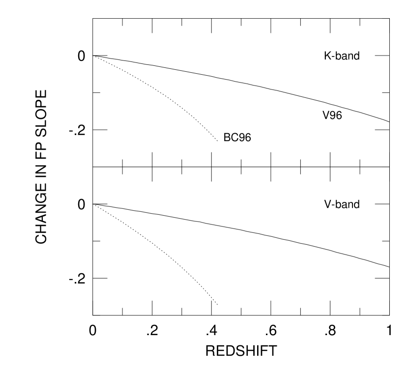
Figure 10: The evolution of the FP with redshift for the two self–consistent model solutions (Vazdekis et al. (1996), V96, Equation 12; Bruzual & Charlot (1996), BC96, Equation 10) which describe the intrinsic physical properties of the early–type galaxy sequence. The cosmology assumed is $(H_{0},\Omega_{0},\Lambda_{0})=(75,0.2,0)$, and the oldest galaxies are taken to be the age of the universe in the present day. The models are arbitrarily cutoff when the youngest galaxies in the early–type galaxy sequence reach an age $<1$ Gyr. The V96 model solution predicts a present–day age spread of 35% along the sequence, while the BC96 model solution predicts a present–day age spread of a factor of two.

The model constructed in §7 also makes specific predictions about the behavior of the FP relations with look-back time or redshift. Age appears to be a significant contributor to the slope of the FP, in the sense that the most luminous elliptical galaxies might be as much as twice as old as the least luminous galaxies. In this model, the slope of the FP should evolve with redshift in the sense that the slope $a$ in $r_{\rm eff}\propto\sigma_{0}^{a}$ will decrease with redshift, since the youngest galaxies at one end of the FP will evolve more quickly than the oldest galaxies at the other end. The specific predictions for the solutions from the Bruzual & Charlot models (Equation 10) and the Vazdekis et al. models (Equation 12) are shown in Figure 10. The evolution of the slope of the FP due to the presence of a dynamical non-homology effect is more complicated. Numerical simulations of dissipationless merging (Capelato, de Carvalho, & Carlberg (1997)) seem to suggest that second and later generation mergers produce a slightly steeper FP than the first generation mergers. Since viewing the FP slope at larger redshifts would then be looking at earlier generations of mergers, their interpretation leads to the prediction that the role of dynamical non-homology should increase with redshift, thereby increasing $d$ and decreasing the slope $a$ with redshift at all wavelengths. This prediction should be treated with caution, however, since it is not clear that the origin of dynamical non-homology effects are in the merging process studied in the numerical simulations.

8.4 Limitations of This Approach

The obvious limitation of this approach is that it still is an empirical description of the observations, not a theoretical construct based on first principles and galaxy formation theory. Nonetheless, it is a first step towards providing detailed, quantitative constraints on the properties that any viable theoretical model for galaxy formation and evolution needs to reproduce.

The only observed property of elliptical galaxies that is not explicitly described by this model is the super–solar enrichment of Mg relative to Fe, although it could certainly be accommodated by the inclusion of recent studies of $\langle$Fe$\rangle$ (such as by Jørgensen (1998) or Trager et al. (1998)) and attempts to model this enrichment (Weiss, Peletier, & Matteucci (1995)). It may be important to reanalyze the galactic wind models (Arimoto & Yoshii (1987)) with these recent super metal–rich, $\alpha$–element enhanced, stellar populations models in a way which embodies the ongoing research into the relative contributions of Type Ia and II supernovae to the chemical enrichment of the host galaxies. This problem is not just a challenge for stellar populations synthesis models, but also for supernova nucleosynthesis, galaxy formation models, and galactic wind models.

A more subtle limitation of this approach is its indirect inclusion of stellar populations gradients, such that the size of these gradients is virtually unconstrained by the model. Clearly, the optimal method of constraining stellar populations gradients is by directly observing them in various colors and line strengths. It is truly surprising that very few new observations have been reported since the review of Peletier (1993), despite the advent of large–format CCD and IR arrays, a sky–subtraction independent parameterization (Sparks & Jørgensen (1993)), and the wealth of photometry that has been obtained from the $U$ to the $K$ bandpasses (Bower, Lucey, & Ellis 1992a ; Jørgensen, Franx, & Kjærgaard 1995a ; Smith et al. (1997); Lucey et al. (1997); Pahre 1998b ). Furthermore, comparing color gradient ratios (between different colors) will provide a strong tool to discriminate between stellar populations gradients and a diffuse component of dust (Wise & Silva (1996)).

9 Summary

The Fundamental Plane slope has been shown to steepen in a systematic way from shorter to longer wavelengths. The methodology presented here shows that changes of the FP slope between bandpasses can be measured accurately by a distance independent construction of the observables. This method is robust and typically reduces the uncertainty of the comparison by a factor of two, thereby allowing for more detailed model comparisons.

This paper presents for the first time a comprehensive model of the changes in global properties of elliptical galaxies that simultaneously accounts for a wide range of observables, namely: (1) the changes in slope of the FP between bandpasses; (2) the slope of the near–infrared FP; (3) the slope of the Mg₂–$\sigma_{0}$ relation; (4) the presence and effects of stellar populations gradients; and (5) the presence of systematic deviations of the internal dynamical structures of elliptical galaxies from a homologous family. The observational constraints imposed by the last element of this model is clearly the weakest point and should be substantially improved upon in the future by obtaining velocity dispersion profiles for large samples of galaxies, such as in a rich cluster. Due to this observational shortcoming, this model does not yet provide highly significant measurements of the individual model parameters defining the variations in age and metallicity from one end of the FP to the other. The model, however, does provide a framework to re-evaluate these parameters as soon as newer and higher quality data become available.

Table 1: Comparison of the Slope of the FP in the Optical and Near–Infrared

Literature	$\lambda$	Fundamental Plane							$D_{n}$–$\sigma_{0}$
Source		$\Delta a$	$\pm$	$c_{K,opt}$	$\pm$	rms	N		$\Delta a$	$\pm$	$c_{K,opt}$	$\pm$	rms	N
						(dex)								(dex)
All Data	$V$	0.18	0.03	0.60	0.07	0.05	239		0.18	0.02	-0.41	0.06	0.04	249
Jørgensen et al. (1996)	$U$	0.51	0.13	0.28	0.30	0.03	20		0.38	0.05	-0.88	0.10	0.03	20
Jørgensen et al. (1996)	$B$	0.32	0.08	0.57	0.17	0.03	25		0.30	0.08	-0.70	0.18	0.03	26
Faber et al. (1989)	$B$	0.19	0.04	0.91	0.10	0.06	145		0.17	0.05	-0.37	0.12	0.05	149
Jørgensen et al. (1996)	$g$	0.21	0.12	0.59	0.28	0.04	26		0.23	0.06	-0.52	0.15	0.03	27
Lucey et al.	$V$	0.23	0.04	0.50	0.10	0.05	83		0.21	0.02	-0.48	0.05	0.03	135
Jørgensen et al. (1996)	$r$	0.17	0.06	0.54	0.14	0.04	55		0.12	0.02	-0.28	0.06	0.03	56
Smith et al. (1997)	$R_{\rm C}$	0.17	0.07	0.45	0.16	0.05	44		0.14	0.02	-0.32	0.04	0.02	44
Scodeggio et al. (1997)	$I_{\rm C}$	0.22	0.10	0.04	0.24	0.04	43		$\cdots$	$\cdots$	$\cdots$	$\cdots$	$\cdots$	$\cdots$

Table 2: Comparison of the Slope of the FP Among Various Optical Bandpasses

Literature	$\lambda_{1}$	Literature	$\lambda_{2}$	Fundamental Plane							$D_{n}$–$\sigma_{0}$
Source 1		Source 2		$\Delta a$	$\pm$	$c_{\lambda_{1},\lambda_{2}}$	$\pm$	rms	N		$\Delta a$	$\pm$	$c_{\lambda_{1},\lambda_{2}}$	$\pm$	rms	N
								(dex)								(dex)
JFK96	$r$	JFK96	$U$	0.22	0.03	0.01	0.07	0.03	45		0.17	0.03	-0.42	0.08	0.02	45
JFK96	$B$	JFK96	$U$	0.13	0.04	-0.15	0.09	0.02	46		0.09	0.03	-0.22	0.07	0.02	46
P96	$B$	P96	$U$	0.13	0.01	-0.13	0.02	0.03	353		$\cdots$	$\cdots$	$\cdots$	$\cdots$	$\cdots$	$\cdots$
P96	$V$	P96	$B$	0.05	0.01	0.19	0.01	0.02	406		$\cdots$	$\cdots$	$\cdots$	$\cdots$	$\cdots$	$\cdots$
JFK96	$r$	JFK96	$B$	0.18	0.04	-0.06	0.10	0.03	36		0.10	0.04	-0.23	0.08	0.02	37
JFK96	$r$	F89	$B$	0.18	0.08	0.00	0.18	0.09	50		0.06	0.04	-0.13	0.09	0.08	52
JFK96	$r$	JFK96	$g$	0.08	0.02	-0.04	0.05	0.02	79		0.09	0.01	-0.20	0.03	0.02	80
JFK96	$r$	L91/97	$V$	0.02	0.03	0.05	0.07	0.02	54		0.03	0.02	-0.04	0.05	0.02	73
P96	$R_{\rm C}$	P96	$V$	0.03	0.01	0.10	0.02	0.01	256		$\cdots$	$\cdots$	$\cdots$	$\cdots$	$\cdots$	$\cdots$
Smi97	$R_{\rm C}$	L91/97	$V$	0.00	0.04	0.18	0.08	0.02	23		0.01	0.02	-0.02	0.04	0.01	24
Sco97	$I_{\rm C}$	L91/97	$V$	0.10	0.06	0.25	0.14	0.04	61		$\cdots$	$\cdots$	$\cdots$	$\cdots$	$\cdots$	$\cdots$
P96	$I_{\rm C}$	P96	$R_{\rm C}$	0.06	0.01	0.24	0.03	0.02	256		$\cdots$	$\cdots$	$\cdots$	$\cdots$	$\cdots$	$\cdots$
Sco97	$I_{\rm C}$	JFK96	$r$	0.17	0.07	-0.00	0.15	0.04	45		$\cdots$	$\cdots$	$\cdots$	$\cdots$	$\cdots$	$\cdots$

References. — The literature sources referenced in this table are as follows. F89: Faber et al. (1989). L91/97: Lucey & Carter (1988), Lucey et al. (1991a,b), and Lucey et al. (1997) J96: Jørgensen et al. (1996). P96: Prugniel & Simien (1996). Smi97: Smith et al. (1997). Sco97: Scodeggio et al. (1997).

Table 3: Variations in Magnitude for Various Bandpasses for the Bruzual & Charlot (1996) and Vazdekis et al. (1996) Models

	Bruzual & Charlot (1996)			Vazdekis et al. (1996)
Bandpass	$\partial m/\partial\log t$	$\partial m/\partial$[Fe/H]		$\partial m/\partial\log t$	$\partial m/\partial$[Fe/H]
	(mag dex-1)	(mag dex-1)		(mag dex-1)	(mag dex-1)
$U$	$+2.934$	$+1.79$		$+2.480$	$+1.50$
$B$	$+2.428$	$+1.12$		$+2.010$	$+1.04$
$V$	$+2.165$	$+0.86$		$+1.755$	$+0.78$
$R_{\rm C}$	$+2.033$	$+0.73$		$+1.629$	$+0.63$
$I_{\rm C}$	$+1.925$	$+0.65$		$+1.540$	$+0.45$
$K$	$+1.480$	$-0.16$		$+1.566$	$-0.13$
Mg2	$+0.174$	$+0.278$		$+0.119$	$+0.199$

Figure 9: Contour plots of $\chi^{2}/\nu$ for the self–consistent model described in the text using the stellar population synthesis models of Vazdekis et al. (1996) as an illustration of the joint confidence of pairs of parameters. In each figure, the $\chi^{2}$ minimum is identified, and two contours delimiting the 95% and 99.7% confidence regions are shown. While age and metallicity have a well–determined joint contribution specified by the “3/2 rule” (as is apparent by their $\chi^{2}/\nu$ valley with slope 3/2), the model parameter $d$, which describes the non-homology contribution, is poorly constrained by the observations. Since age and $d$ are jointly constrained by the slope of the $K$–band FP (Equation 12), better independent constraints on $d$ will further limit the allowed parameter space for age and thus further break the age–metallicity degeneracy.

References

- Arimoto & Yoshii (1987) Arimoto, N., & Yoshii, Y. 1987, A&A, 173, 23
- (2) Bower, R. G., Lucey, J. R., & Ellis, R. S. 1992a, MNRAS, 254, 589
- (3) Bower, R. G., Lucey, J. R., & Ellis, R. S. 1992b, MNRAS, 254, 601
- Bruzual & Charlot (1996) Bruzual, A. G., & Charlot, S. 1996, in preparation
- Burkert (1993) Burkert, A. 1993, A&A, 278, 23
- Burstein & Heiles (1982) Burstein, D., & Heiles, C. 1982, AJ, 87, 1165
- Busarello et al. (1997) Busarello, G., Capaccioli, M., Capozziello, S., Longo, G., & Puddu, E. 1997, A&A, 320, 415
- Caon, Capaccioli, & D’Onofrio (1993) Caon, N., Capaccioli, M., & D’Onofrio, M. 1993, MNRAS, 265, 1013
- Capelato, de Carvalho, & Carlberg (1995) Capelato, H. V., de Carvalho, R. R., & Carlberg, R. G. 1995, ApJ, 451, 525
- Capelato, de Carvalho, & Carlberg (1997) Capelato, H. V., de Carvalho, R. R., & Carlberg, R. G. 1997, in Galaxy Scaling Relations: Origins, Evolution, and Applications, Proceedings of the Third ESO–VLT Workshop, eds. L. N. da Costa & A. Renzini (Springer–Verlag: Berlin), 331
- de Carvalho & Djorgovski (1992) de Carvalho, R. R., & Djorgovski, S. 1992, ApJ, 389, L49
- Charlot, Worthey, & Bressan (1996) Charlot, S., Worthey, G., & Bressan, A. 1996, ApJ, 457, 625
- Ciotti, Lanzoni, & Renzini (1996) Ciotti, L., Lanzoni, B., & Renzini, A. 1996, MNRAS, 282, 1
- Couture & Hardy (1988) Couture, J., & Hardy, E. 1988, AJ, 96, 867
- Davies et al. (1983) Davies, R. L., Efstathiou, G., Fall, S. M., Illingworth, G., & Schechter, P. L. 1983, ApJ, 266, 41
- Davies, Sadler, & Peletier (1993) Davies, R. L., Sadler, E. M., & Peletier, R. F. 1993, MNRAS, 262, 650
- Djorgovski & Davis (1987) Djorgovski, S., & Davis, M. 1987, ApJ, 313, 59
- Djorgovski & Santiago (1993) Djorgovski, S., & Santiago, B. X. 1993, in proceedings of the ESO/EIPC Workshop on Structure, Dynamics, and Chemical Evolution of Early–Type Galaxies, ed. J. Danziger, et al., ESO publication No. 45, 59
- Dressler et al. (1987) Dressler, A., Lynden-Bell, D., Burstein, D., Davies, R. L., Faber, S. M., Terlevich, R. J., & Wegner, G. 1987, ApJ, 313, 42
- Ellis et al. (1997) Ellis, R. S., Smail, I., Dressler, A., Couch, W. J., Oemler, A., Jr., Butcher, H., & Sharples, R. M. 1997, ApJ, 483, 582
- Faber & Jackson (1976) Faber, S. M., & Jackson, R. E. 1976, ApJ, 204, 668
- Faber et al. (1989) Faber, S. M., Wegner, G., Burstein, D., Davies, R. L., Dressler, A., Lynden-Bell, D., & Terlevich, R. J. 1989, ApJS, 69, 763
- Franx, Illingworth, & Heckman (1989) Franx, M., Illingworth, G., & Heckman, T. 1989, AJ, 98, 538
- Fritze-v. Alvensleben & Burkert (1995) Fritze-v. Alvensleben, U., & Burkert, A. 1995, A&A, 300, 58
- Gorgas, Efstathiou, & Aragón Salamanca (1990) Gorgas, J., Efstathiou, G., & Aragón Salamanca, A. 1990, MNRAS, 245, 217
- Graham & Colless (1997) Graham, A., & Colless, M. 1997, MNRAS, 287, 221
-