The mass and radius of the M dwarf companion to GD 448

Abstract

We present spectroscopy and photometry of GD 448, a detached white dwarf – M dwarf binary with a period of 2$\stackrel{{\scriptstyle h}}{{\textstyle.}}$47. We find that the Na I 8200Å feature is composed of narrow emission lines due to irradiation of the M dwarf by the white dwarf within broad absorption lines that are essentially unaffected by heating. Combined with an improved spectroscopic orbit and gravitational red shift measurement from spectra of the ${\rm H}\alpha$ line, we are able to derive masses for the white dwarf and M dwarf directly ($0.41\pm 0.01$$M_{\odot}\,$and $0.096\pm 0.004$$M_{\odot}\,$, respectively). We use a simple model of the Ca II emission lines to establish the radius of the M dwarf assuming the emission from its surface to be proportional to the incident flux per unit area from the white dwarf. The radius derived is 0.125 $\pm$ 0.020 $R_{\odot}\,$. The M dwarf appears to be a normal main-sequence star in terms of its mass and radius and is less than half the size of its Roche lobe. The thermal timescale of the M dwarf is much longer than the cooling age of the white dwarf so we conclude that the M dwarf was unaffected by the common-envelope phase. The anomalous width of the ${\rm H}\alpha$ emission from the M dwarf remains to be explained, but the strengh of the line may be due to X-ray heating of the M dwarf due to accretion onto the white dwarf from the M dwarf wind.

1 Introduction

GD 448 ($=$ WD 0710$+$741, LP034$-$185) was shown by Marsh & Duck (1996; MD96 hereafter) to be a detached white dwarf – M dwarf binary with a period of 2$\stackrel{{\scriptstyle h}}{{\textstyle.}}$47. This is the shortest period known for such a binary and places it in the centre of the “period gap” from 2 to 3 hours in which very few cataclysmic variable stars (semi-detached white dwarf – main-sequence binaries) are found. From the cooling age of the white dwarf, MD96 found that GD 448 was born in the period gap and had never been a cataclysmic variable star. They also found that the ${\rm H}\alpha$  emission line from the heated face of the M dwarf is much broader than expected. Since the thermal timescale of the M dwarf is much longer than the cooling-age of the white dwarf the radius of the M dwarf in GD 448 is essentially unchanged from the radius at the end of the common-envelope phase. This enables us to study the effect of the common-envelope phase on the M dwarf. Unfortunately, the data of MD96 were of insufficient quality to establish the radius of the M dwarf.

In this paper we present V and I band lightcurves of GD 448 and much improved spectroscopy which has enabled us to determine the radius of the M dwarf in GD 448 and to improve the mass estimates for both components.

2 Observations

2.1 Spectroscopy

We observed GD 448 over four nights (11-14 January 1996) using the double-beam spectrograph ISIS on the 4.2m William Herschel Telescope. Data were obtained over three nights in variable conditions. We used the R1200R grating in the blue arm and the R600R grating in the red-arm with TEK CCD detectors to obtain spectra covering 400Å around ${\rm H}\alpha$  at a dispersion of 0.4Å per pixel and an 800Å region covering the Na I 8200Å doublet and Ca II infrared triplet at a dispersion of 0.8Å per pixel. A total of 161 spectra were obtained in each spectral region. A 0.9″ wide slit which projected onto 1.6 pixels at the detectors was used to ensure accuracy in the measured radial velocities. Exposure times were 300s – 500s. Optimal extraction was used to extract spectra from our CCD images. All the observation were interspersed with observations of a copper-argon arc at least every 40 minutes and before and after every re-pointing of the telescope. Spectra of the arc were extracted at the same detector position as the object spectra. The wavelength scale determined from a polynomial fit to measured arc line positions was interpolated in time for the object spectra.

The spectra were flux calibrated using spectra of BD$+26$ 2606 (Oke 1983) to correct for the wavelength-dependent instrument sensitivity. No correction for slit losses was attempted so the spectra have an arbitrary absolute flux scale. Telluric features in the red-arm data were removed using the technique of Wade & Horne (1988). The rapidly rotating B-type star HD 84937 was used to determine the telluric absorption spectrum. The removal is naturally imperfect as the strength of the telluric absorption had to be estimated from the airmass at which each spectrum of GD 448 was observed.

2.2 Photometry

We used the 1m Jacobus Kapteyn telescope to obtain V and I band CCD images of GD 448. The detector used was a TEK CCD with $1024^{2}$ pixels giving an image scale of 0.34″ per pixel. Observations were obtained during the first 1-2 hours of the nights 28 March to 2 April 1996. A total of 84 useful images were obtained with the I filter and 30 in the V filter. Normalized average images of the twilight sky were used to apply flat-field corrections to all the images.

Table 1: Position of GD448 and comparison stars Coordinates are equinox 2000.0, epoch 1996.24 and are accurate to a few arcseconds.

Star	RA	Dec
GD 448	$07^{h}17^{m}09.6^{s}$	$+74\mbox{${}^{o}$}00\mbox{${}^{\prime}$}42\mbox{${}^{\prime\prime}$}$
C1	$07^{h}17^{m}03.9^{s}$	$+74\mbox{${}^{o}$}03\mbox{${}^{\prime}$}32\mbox{${}^{\prime\prime}$}$
C2	$07^{h}16^{m}41.3^{s}$	$+74\mbox{${}^{o}$}00\mbox{${}^{\prime}$}23\mbox{${}^{\prime\prime}$}$

Figure 1: The V and I lightcurves of GD 448 (upper and lower panels, resp.).

We used profile fitting to determine differential magnitudes of 8 stars in the images including GD 448, all of which were used to determine the shape of the profile to be used in each image. After careful inspection of the images and the resulting magnitudes of these stars we chose the comparison star C1 and a check star C2 ($\equiv$ GSC 4372 00331) whose positions are given in table 1. The positions of these stars and GD 448 were measured from our images using positions for 5 Hubble Guide Star Catalogue stars to establish the linear astrometric solution. The magnitude difference between these stars is seen to be constant to within $\approx 0\mbox{$\stackrel{{\scriptstyle m}}{{\textstyle.}}$}01$. The lightcurve of GD 448 with respect to C1 is shown in Fig. 1 where the phase has been calculated using the ephemeris given below. The I band lightcurve clearly shows the effect of the irradiation of the M dwarf by the white dwarf. The incomplete coverage of the V lightcurve makes it difficult to judge whether the variabilty at this wavelength is due to irradiation, although a cosine function gives a good fit to the incomplete lightcurve and suggests the amplitude of the V lightcurve is half that of the I lightcurve.

3 Results

3.1 The Ca II triplet

Figure 2: The measured radial velocities for the Ca II triplet emission lines (upper panel) and adopted fit.

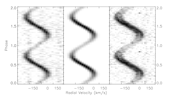
Figure 3: Trailed and phase-binned spectra of the Ca II 8542Å line (left panel), the model spectra for the simple model of Ca II emission and the adopted value $f$ (middle panel) and the ${\rm H}\alpha$ emission line after subtraction of the white dwarf absorption (right panel).

The red-arm spectrum shows the Ca II triplet emission lines seen by MD96. These are of roughly equal strength and show sinusoidal variations of intensity and Doppler shift with phase. This can be seen in Figs. 2, 3 and 6, which are described in more detail below.

Table 2: The parameters of the Gaussian profiles used to fit the Ca II emission lines.

parameter	Value	Notes
FWHM(${\rm km\,s}^{-1}$)	$58.6\pm 0.5$	Mean width of lines.
		No phase variation seen.
h(8662)/h(8542)	$0.830\pm 0.010$	Ratio of heights
h(8498)/h(8542)	$0.708\pm 0.007$	Ratio of heights
$A^{1}$	$0.409\pm 0.002$
$B^{1}$	$-0.267\pm 0.003$
1: Fit to height dependence on phase $\phi$, $h=A+B\cos(\phi)$

We used a series of Gaussian fits to individual spectra to measure the radial velocity of the Ca II triplet in a similar manner to MD96. The spectra are normalised to a continuum value near the Ca II lines determined from a cosine fit to the I-band lightcurve. We find $C_{I}=1-0.03\cos(\phi)$, where $C_{I}$ is the continuum value and $\phi$ is the orbital phase in radians, phase zero being times at which the M-star is closest to the Earth. The ratio of the heights of the Ca II lines was held fixed at a value determined from a previous fit and the variation of the height of the lines with phase was set by a fit to the measured individual heights of the form $A+B\cos(\phi)$. We detected no variation of the width of the lines with phase so this height variation has the same form as the equivalent width variation seen in Fig. 6. Values of the parameters used in the fit are given in table 2. The reduced chi-squared values for the fits were typically 0.9 – 1.1.

Table 3: Circular orbit fits

Spectral line(s)	$\gamma(\mbox{${\rm km\,s}^{-1}$})$	$K(\mbox{${\rm km\,s}^{-1}$})$
Ca II IR triplet emission	$-40.8\pm 0.35$	$123.1\pm 0.4$
${\rm H}\alpha$ absorption	$-24.2\pm 0.6$	$-33.5\pm 0.9$
${\rm H}\alpha$ emission	$-38.1\pm 0.4$	$125.4\pm 0.6$
Na I 8200Å absorption	$-38.6\pm 1.5$	$142\pm 3$
Na I 8200Å emission	”	$120\pm 3$
8800.3Å  absorption	—	$148\pm 5$

We used a periodgram of our radial velocity measurements combined with those of MD96 to confirm the orbital period, $P$. The cycle count between the two data sets is confirmed by the lightcurve. From the sine curve fit of the form $\gamma_{\rm M}+K^{\rm Ca\,II}_{\rm M}\sin(\phi)$ to the combined radial velocity data shown in Fig. 2 we find the following ephemeris:

$${\rm HJD}(T_{0})=2450094.69006(7)+0.10306437(7)E,$$

where figures in parentheses are 1-$\sigma$ uncertainties in the final digit and $T_{0}$ refers to dates at which the M-star is closest to the Earth. The values of $\gamma_{\rm M}$ and $K^{\rm Ca\,II}_{\rm M}$ determined from this fit are given in table 3. This ephemeris agrees with that of MD96 once a superfluous digit in their quoted period is accounted for.

Figure 4: The average red-arm spectrum after removal of the Ca II radial velocity Doppler shift.

The average red-arm spectrum after subtraction of the Doppler shift due to this orbit is shown in Fig. 4. In addition to the Ca II triplet, there are several other emission lines visible. Some of these are labelled with tentative identifications which are based on a simple model of emission from an optically thin gas with a range of effective temperature around 5000 - 10 000K. Also visible is the Na I 8200Å feature, which is distorted by the averaging process, as well TiO and other absorption features.

3.2 The Na I doublet.

Table 4: The parameters of the Gaussian profiles used to fit the Na I doublet. Parameters in bold type are fixed quantities.

Wavelength(Å)	8183.3	8194.8	8183.3	8194.8	$8207.5\pm 0.4$
FWHM(Å)1	$3.3\pm 0.2$	$3.8\pm 0.2$	$1.8\pm 0.1$		$2.5\pm 0.9$
Height	$-0.079\pm 0.004$	$-0.073\pm 0.004$	$1.07\pm 0.09$	$0.99\pm 0.08$	$-0.010\pm 0.002$
$A$	—	—	$0.066\pm 0.003$	$0.057\pm 0.003$	—
$B$	—	—	$-0.038\pm 0.004$	$-0.048\pm 0.004$	—

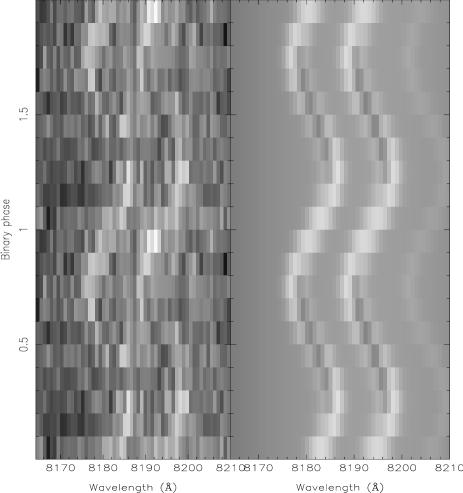
Figure 5: Trailed and phase-binned spectra around the Na I 8200Å absorption line (left panel) and the best fit using multiple Gaussian fits (right panel).

We experimented with several models to account for the variation with phase of the Na I doublet. The most successful and easiest to interpret is that of narrow emission lines, similar to the Ca II emission lines, with semi-amplitude $K^{\rm Na\,I}_{\rm M}$ superimposed on broad absorption lines which are constant with phase, i.e., with the same semi-amplitude as the centre-of-mass of the M dwarf, $K_{\rm M}$. To measure the values of $K^{\rm Na\,I}_{\rm M}$ and $K_{\rm M}$ we used a fitting method similar to Moran et al. (1997), in which a simultaneous Gaussian fit to all the spectra is used to determine the orbital parameters. A single Gaussian was used to model each emission and absorption component for both Na I lines and a third Gaussian was used to account for weak absorption line nearby. The parameters of these Gaussians are given in table 4. The variation in height of the emission lines was established from a cosine fit to measured individual heights. note that this is similar to the variation seen in the Ca II emission lines. The reduced chi-squared value of the final fit is 1.05 (9285 data points) which is acceptable given the difficulties in removing telluric features in this region. The observed Na I line spectra and fits have been coadded into phase bins to produce the trailed spectra shown in Fig. 5 .

We were able to confirm the value of $K_{\rm M}$ using the absorption line seen near 8800Å in Fig. 4, which we tentatively identify as FeI 8801.8Å. We used a fit of a single Gaussian to this line to determine $K_{\rm M}$. The line shows no variation of depth or width with phase and is unaffected by telluric features. The nearby MgI emission line was accounted for in the fit and was found to behave in a similar way to the Ca II lines. We find $K_{\rm M}=148\pm 5\mbox{${\rm km\,s}^{-1}$}$, in good agreement with the value determined from Na I. The weighted average of the two values is $144\pm 3\mbox{${\rm km\,s}^{-1}$}$, which is our adopted value for $K_{\rm M}$.

3.3 The ${\rm H}\alpha$ line.

Table 5: The parameters of the Gaussian profiles used to fit ${\rm H}\alpha$.

Component	FWHM(Å)	Height
Emission line	$2.08\pm 0.02$	$1.030\pm 0.0006^{a}$
Absorption component 1	$1.321\pm 0.034$	$-0.175\pm 0.002$
Absorption component 2	$6.87\pm 0.30$	$-0.070\pm 0.002$
Absorption component 3	$28.36\pm 0.90$	$-0.109\pm 0.003$
Absorption component 4	$67.35\pm 2.41$	$-0.117\pm 0.003$
Absorption component 5	$153.6\pm 4.40$	$-0.074\pm 0.003$
$a$: The actual height of the emission is given by this value
multiplied by the cosine variation described in the text.

The contribution from the M dwarf to the continuum near ${\rm H}\alpha$ is negligible so the continuum was set to unity using a linear fit to the continuum 8000-8500${\rm km\,s}^{-1}$either side of the line. We used five Gaussian profiles to model the absorption profile and a single Gaussian profile to measure the emission feature. A series of fits were used to establish the height variation of the emission line, which is similar to the Ca II emission. We also established the widths and heights of the Gaussian profiles given in table 5, and the apparent systemic radial velocity, $\gamma_{\rm M}$ and semi-amplitude, $K^{\rm\mbox{${\rm H}\alpha$}}_{\rm M}$ of the ${\rm H}\alpha$ emission line given in table 3 using a simultaneous fit to all the spectra.

We were concerned that the variation of the ${\rm H}\alpha$ emission line might affect our estimates of $\gamma_{\rm WD}$ and $K_{\rm WD}$ – the apparent systemic radial velocity and semi-amplitude of the white dwarf. To avoid this we excluded a region on either side of the predicted emission line position from the fitting process with similar width to the FWHM of the emission line ($\sim 100\mbox{${\rm km\,s}^{-1}$}$). We then used a simultaneous fit to all the spectra to measure the $\gamma_{\rm WD}$ and $K_{\rm WD}$. The results vary slightly depending on the width of the excluded region, and this additional uncertainty has been included in the adopted values shown in table 3.

Figure 6: Variation of the equivalent width of the ${\rm H}\alpha$ (filled circles) and Ca II 8542Å (crosses) emission lines with phase. Solid lines are fits of the form $A+B\sin(\phi)+C\sin(2\phi)$. The dotted line is the best fit for an optically thick model to the Ca II 8542Å line.

Our fit to the white dwarf absorption line was used to subtract the contribution of the white dwarf from the ${\rm H}\alpha$ line. The remaining M dwarf emission line spectra were coadded in phase-bins to produce the trailed spectra shown in Fig. 3. The equivalent width variation of this line is shown in Fig. 6. It is obvious from Fig. 3 that the ${\rm H}\alpha$ emission is much wider than the Ca II emission lines, a feature noted by MD96. Less obvious but still visible is the double-peaked shape of the ${\rm H}\alpha$ emission near phases 0.25 and 0.75. These anomalies are discussed in more detail in section 5.

3.4 The mass of the white dwarf and the M dwarf.

Table 6: Summary of the parameters of GD 448.

Parameter	white dwarf	M dwarf
Mass ($M_{\odot}\,$)	$0.41\pm 0.01$	$0.096\pm 0.004$
Radius($R_{\odot}\,$)	$0.018$	0.125 $\pm$ 0.02 $R_{\odot}\,$
Inclination(o)	$29.3\pm 0.7$
Period ($d$)	0.10306437

The measured values of $K_{\rm WD}$, $K_{\rm M}$ and the orbital period lead directly via Kepler’s laws to $M_{\rm WD}\sin^{3}i$ and $M_{\rm M}\sin^{3}i$, where $M_{\rm WD}$ is the mass of the white dwarf, $M_{\rm M}$ is the mass of the M dwarf and $i$ is the inclination. The actual mass of the white dwarf can be established from the gravitational red shift and the mass – radius relation for white dwarfs. To the difference $(\gamma_{\rm WD}-\gamma_{\rm M})=13.9\pm 0.6\mbox{${\rm km\,s}^{-1}$}$ measured from the ${\rm H}\alpha$ line must be added corrections for the red shift of the M dwarf (0.5${\rm km\,s}^{-1}$) and the difference in transverse Doppler shifts (0.1${\rm km\,s}^{-1}$) as described by MD96, as well as for the potential at the M dwarf due to the white dwarf (0.35${\rm km\,s}^{-1}$) and vice versa (-0.08${\rm km\,s}^{-1}$), a correction which MD96 omitted. The mass of the white dwarf is then determined from the model cooling curves for low-mass helium white dwarfs of Althaus & Benvenuto (1997). For white dwarfs with an effective temperature of 19 000K and a mass near 0.4$M_{\odot}\,$, we find the mass in solar masses is related to the gravitational red shift, $v_{g}$, in ${\rm km\,s}^{-1}$ by $M=0.181+0.0157v_{g}$. The inclination can then be determined using equation (1) of MD96. The corrections to the gravitational red shift depend slightly on the assumed values of $i$ and so an iterative scheme is used to find consistent values for all the parameters. The dependence of the results on the assumed radius of the M dwarf is negligible for any reasonable estimate. The inclination and masses derived are given in table 6. The radius of the white dwarf is also given, although no error is quoted as this is strongly correlated with the uncertainty in the mass.

4 Determination of the radius of the M dwarf from the Ca II triplet.

The Ca II emission in GD448 is due to emission from the heated face of the M dwarf so $K^{\rm Ca\,II}_{\rm M}$ is lower than $K_{\rm M}$. The correction $\Delta K=K_{\rm M}-K^{\rm Ca\,II}_{\rm M}$ depends on the pattern of the emission over the surface of the M dwarf and its radiative properties (e.g., optical depth, limb darkening) as well as the geometry of the system. The only free parameter in the system geometry is the filling factor of the M dwarf, $f$, the ratio of the radii of the M dwarf and its Roche lobe measured from the centre-of-mass to the inner Lagrangian point. A value of $f=1$ corresponds to a Roche lobe filling star. The other parameters (e.g., inclination, mass ratio) have been derived in section 3.4 above.

For our model of the emission from the M dwarf, we assumed a source function of the form $1+\epsilon\tau\mu$ where $\tau$ is the optical depth along the line of sight and $\mu$ is the cosine of the angle between our line of sight and the normal to the surface. The dependence of the emission line flux from a point on the star, $F$, with viewing angle then has the form:

$$F\propto(1+\epsilon\cdot\mu)(1-e^{-\tau_{0}/\mu})-\epsilon\cdot\tau_{0}e^{-\tau_{0}/\mu},$$

where $\tau_{0}$ is the vertical optical depth through the emitting region, which is assumed to be constant over the surface of the star. In the optically thick case ($\tau_{0}\gg 1$), $\epsilon$ is related to the standard linear limb darkening parameter which is given by $\epsilon/(1+\epsilon)$ when $\epsilon$ is positive. In cases where $\epsilon$ is negative, i.e., source function increasing with height, as might be expected in the case of an irradiated atmosphere, $\tau_{0}$ must be less than $-1/\epsilon$ to avoid negative source function values.

We used numerical integration over a model star defined by a surface of constant Roche potential to predict emission line strengths and radial velocities for various values of $f$, $\epsilon$ and $\tau_{0}$ assuming the emission line strength to be proportional to the incident flux per unit area from the white dwarf. These were calculated at the same phases as the observed data and given the same weighting in a sine fit that was used to calculate $\Delta K$. This has an almost linear dependence on $f$ and so it is very easy to find $f$ which gives the correct value of $\Delta K$.

A further constraint on our model of the Ca II emission comes from the lightcurve of the Ca II lines, i.e., the variation of equivalent width with phase. By fitting a function of the form $A+B\sin(\phi)+C\sin(2\phi)$ to the observed equivalent width variation, we find $C/B=-0.02\pm 0.02$. This ratio describes the magnitude of any non-sinusoidal component of the lightcurve (i.e., its shape) independent of any zero-point or scaling applied. For each value of $\epsilon$ and $\tau_{0}$ used, the predicted equivalent widths for the optimum filling factor $f_{0}$ were calculated at the same phases as the observed data and given the same weighting in a fit of the same function. The ratio $C/B$ from these fits rules out models with values of $\tau_{0}\mathrel{\mathchoice{\vbox{\offinterlineskip\halign{\hfil$\displaystyle#$\hfil\cr>\cr\sim\cr}}}{\vbox{\offinterlineskip\halign{\hfil$\textstyle#$\hfil\cr>\cr\sim\cr}}}{\vbox{\offinterlineskip\halign{\hfil$\scriptstyle#$\hfil\cr>\cr\sim\cr}}}{\vbox{\offinterlineskip\halign{\hfil$\scriptscriptstyle#$\hfil\cr>\cr\sim\cr}}}}1.0$. These models show a non-sinusoidal component that is much larger than that observed ($C/B\sim 0.1$), i.e., they are the wrong shape. This is shown in Fig. 6.

Figure 7: A cross section through the orbital plane of GD 448 showing the relative sizes of the white dwarf (filled circle) and the M dwarf (partially hatched) with its Roche lobe (dashed lines). The hatched region of the M dwarf shows approximately where the Ca II and ${\rm H}\alpha$ arise. The $+$ symbol marks the centre of mass of the system and the $\times$ symbol the centre of mass of the M dwarf. The axes are in units of the orbital separation ($r_{x}$ and $r_{y}$) and the amplitude of the sine and cosine components of projected radial velocity ($K_{x}$ and $K_{y}$).

The values of $f_{0}$ found for valid values of $\tau_{0}$ vary from 0.46 ($\tau_{0}\ll 1$) to 0.49 ($\tau_{0}=1$) whatever the value of $\epsilon$. The uncertainty in $K_{\rm M}$ leads to an further uncertainty of 0.06 in $f_{0}$. The absolute radius of the M dwarf is then 0.125 $\pm$ 0.015 $\pm$ 0.005 $R_{\odot}\,$, where the uncertainties quoted are the random error inherited from $K_{\rm M}$ and the systematic error due to the range of $f_{0}$ values, respectively. The combination of systematic and random uncertainties is a moot point, but the result cannot be worse than a simple linear addition and so we will adopt a value of 0.125 $\pm$ 0.02 $R_{\odot}\,$. The relative sizes of the white dwarf, the M dwarf and the Roche lobe of the M dwarf are shown in Fig. 7.

Figure 8: GD 448 in the mass-radius plane (filled circle) compared to other low-mass stars and brown dwarfs from Clemens et al. (open circles).

The position of the M dwarf in the mass–radius plane is shown in Fig. 8. Also shown in Fig. 8 for comparison are masses and radii for other M dwarfs given by Clemens et al. (1997). Their masses are based on their revised empirical color–luminosity relation and the luminosity–mass relation of Henry & McCarthy(1993) based on 37 visual binaries. The radii are derived from their updated colour–temperature and colour–bolometric correction relations based on a volume limited sample of 127 M dwarfs. The agreement between their indirect method and our more direct method is quite satisifactory.

5 Discussion.

Comparing the position of GD 448B in the mass–radius plane to those of other M dwarfs, we see that it appears to be a perfectly normal main-sequence M dwarf. The thermal timescale for the M dwarf ($3\times 10^{9}$y) is much longer than the cooling age of the white dwarf ($5\times 10^{7}$y), so the radius will not have changed significantly since the common-envelope phase. The argument of MD96 which suggests that GD 448 was born in the period gap, i.e., has never been a CV, is not affected by anything presented here.

The anomalous width of the ${\rm H}\alpha$ emission line is particularly strange given that its intensity variation with phase and radial velocity semi-amplitude are almost identical to the much narrower Ca II emission lines. For example, from a fit of the form $A+B\sin(\phi)+C\sin(2\phi)$ to the equivalent width variation of the Ca II 8542Å line shown in Fig. 6 we find, $B/A=-0.68\pm 0.01$ and $C/B=-0.03\pm 0.02$. The other Ca II lines give similar results. For the ${\rm H}\alpha$ emission we find the remarkably similar values $B/A=-0.71\pm 0.02$ and $C/B=-0.05\pm 0.02$, i.e., the Ca II and ${\rm H}\alpha$ emission lines have nearly identical amplitudes and shapes. This appears to rule out any broadening mechanism requiring a distribution of ${\rm H}\alpha$ emitting material much different from the Ca II emitting region, e.g., photospheric emission.

Our favoured explanation for the shape of the ${\rm H}\alpha$ line is some broadening mechanism (e.g., natural damping or Stark broadening) within an optically thick medium. This is at variance with the results of our simple model for the emission of Ca II which appears to rule out emission from an optically thick gas. However, our simple model is not complete as it does not account for any variation of the optical depth over the surface of the M dwarf, nor for the finite geometrical depth of the emitting layer. In the case of emission from an optically thin gas, the emission line strengths are expected to be proportional to the oscillator strengths of the transitions. In the case of the Ca II lines, these ratios are Ca II 8498 : Ca II 8542 : Ca II 8662 = 1 : 9 : 5. The observed ratio of the emission line strengths is 1 : 1.4 : 1.2, which suggest that at least some part of that emission is due to optically thick material. The double-peaked shape of the ${\rm H}\alpha$ emission might then be explained as self-absorption of the line. Clearly, more detailed modeling would be required to demonstrate that these suggestions are feasible, but if they do adequately explain the shape of the ${\rm H}\alpha$ and Ca II emission lines, these lines would then be giving information on the density and temperature structure within the emitting region.

If our assumption that the pattern of Ca II emission is proportional to the irradiating flux is wrong, it might seem possible to explain the width of ${\rm H}\alpha$ as rotational broadening of an intrinsically narrow line. This would then require a very odd distribution of ${\rm H}\alpha$ and Ca II emission over the surface M dwarf to explain the shape of the ${\rm H}\alpha$ line. In fact, we used a very general model of the ${\rm H}\alpha$ emission in which the pattern of emission over the surface of the M dwarf was allowed to vary independently at every grid point, each of which emits a narrow line. The model includes the effects of orbital phase smearing and the instrumental resolution. We then attempted to use a maximum entropy reconstruction to determine a pattern of emission that produced emission lines consistent with the data, but were unable to find any such pattern for any value of $f$. This is a similar problem to that found by Rutten & Dhillon (1994) in the case of the cataclysmic variable star DW UMa, although that case is complicated by the presence of an accretion disc.

The photometry for GD448 has only been used to confirm the correct orbital period for the system and to normalise the continuum value for the red-arm spectra. A simple model of the irradiation shows that the amplitude of the lightcurve is consistent with that which would be expected from an irradiated star, but given the uncertainties in the heating mechanism and the small amplitude of the modulation this gives no constraint on the system geometry in practice.

The problem of the strength of the ${\rm H}\alpha$ emission discussed by MD96 remains and is made worse by the small radius for the M dwarf derived here. Briefly, there is insufficient radiation below the Lyman limit from the white dwarf incident at the M dwarf surface to produce the observed emission line strength by photoionisation of hydrogen. A similar problem has been identified for the detached white dwarf – M dwarf binaries PG1026+002 (Saffer et al., 1993) and WD2256+249 (Schmidt et al., 1995). MD96 suggest that chromospheric activity may excite hydrogen atoms to the n=2 level, from where they are ionised.

An alternative explantion comes from the possibility of accretion onto the white dwarf from the M dwarf wind, a process seen in the white dwarf – K dwarf detached binary V471 Tau (Mullan et al. 1991). The resulting irradiation from the soft X-rays produced would be sufficient to produce the observed ${\rm H}\alpha$ flux for mass-loss rates only a few times greater than the Solar mass-loss rate. To calculate the ${\rm H}\alpha$ flux, we first used the mass – colour – absolute-magnitude relations for M dwarfs from Clemens et al. (1998) to find (V-I)=$4.0\pm 0.1$ and $\mbox{$M_{\mbox{\scriptsize V}}\,$}=16.2\pm 0.3$. We then used $M_{\mbox{\scriptsize V}}\,$=10.15 for the white dwarf (Bergeron et al., 1992) and (V-I)=$-0.204$ for a hydrogen-rich white dwarf of 19 000K (Bergeron et al.1995) to predict a contribution of 15%$\pm$3% from the M dwarf in the I band ($\sim 8200\AA$). This is in perfect agreement with the estimate of MD96. We used (R-I)=2.16 for the M dwarf (Bessel, 1991), which implies a spectral type of M5.5 – M6, and (R-I)=-0.11 for the white dwarf (Bergeron et al. 1995) to find a contribution of 2.2%$\pm$0.7% from the M dwarf in the R band ($\sim 7000$Å). The peak equivalent width of the ${\rm H}\alpha$ emission relative to the combined continuum is 1.0Å so the true equivalent width of the emission is $\sim 45$Å. The zero-point of the R-band magnitude scale for M dwarfs is approximately $30\times 10^{-13}$ W m${}^{-2}{\rm\AA}^{-1}$ (Allard & Hauschildt. 1995) and the V magnitude of GD 448 is 14.97 (Bergeron et al., 1992) so the observed ${\rm H}\alpha$ flux from the M dwarf is $\approx 3\times 10^{-18}$W m^-2. For the purposes of this discussion we can assume this ${\rm H}\alpha$ flux is radiated isotropically from the M dwarf, in which case the luminosity in ${\rm H}\alpha$ of the M dwarf is $3\times 10^{20}$W. If all the X-radiation emitted from the white dwarf intercepted by the M dwarf (1.5% for isotropic emission) is re-processed as ${\rm H}\alpha$ emission, the X-ray luminosity of the white dwarf is $2\times 10^{22}$W. The mass accretion rate required to provide this energy is $\sim 1\times 10^{-14}\mbox{$M_{\odot}\,$}{\rm y}^{-1}$. The efficiency of Bondi-Hoyle accretion from the M dwarf wind is expected to be quite high ($\sim 20$%, Mullan et al. 1991). Furthermore, models of X-ray heating of dwarf M-star chromospheres suggest that perhaps half of the energy is re-emitted as Balmer emission if the X-rays are absorbed high in the atmosphere (Cram 1982). The total mass-loss rate required to produce ${\rm H}\alpha$ could then be as low as $\sim 1\times 10^{-13}\mbox{$M_{\odot}\,$}{\rm y}^{-1}$ – comparable to the Solar mass-loss rate and much lower than the observed mass-loss rate in other M dwarfs (Mullan et al. 1992). The observed X-ray flux in this scenario would be $\sim 2\times 10^{-16}{\rm W\,m}^{-2}\equiv 2\times 10^{-13}{\rm ergs\,s}^{-1}{\rm cm}^{-2}$, which is well within the capabilities of the current generation of X-ray satellites.

6 Conclusion.

Extensive analysis of spectra covering the ${\rm H}\alpha$ line, the Ca II triplet and the NaI doublet from GD448 have enabled us to determine the mass and radius of the M dwarf companion to the white dwarf GD 448. Its position in the mass-radius relation places it squarely on the main-sequence. This suggests that the common envelope phase had little effect on the structure of the M dwarf. The anomalous width of the ${\rm H}\alpha$ emission from the M dwarf remains to be explained. The anomalous strength of the ${\rm H}\alpha$ line may be due to X-ray heating of the M dwarf due to accretion onto the white dwarf from the M dwarf wind.

References

- [1] Allard F., Hauschildt P. H., 1995, ApJ, 445, 433
- [2] Althaus L. G., Benvenuto O. G., 1997, ApJ, 477, 313
- [3] Bergeron P., Saffer R. A., Liebert J.,1992, ApJ, 394,228
- [4] Bergeron P., Wesemael F., Beauchamp A., 1995, PASP, 107, 1047
- [5] Bessel M. S., 1991, AJ, 101, 662
- [6] Clemens J. C., Reid I. N., Gizis J. E., O’Brien M. S., 1998, ApJ, 496, 352
- [7] Cram L. E., 1982, ApJ, 253, 768
- [8] Henry T. J., McCarthy D. W. 1993, AJ, 106, 773
- [9] Marsh T. R., Duck S. R, 1996, MNRAS, 278, 565 (MD96).
- [10] Moran C., Marsh T. R., Bragaglia A., 1997, MNRAS, 288, 538
- [11] Mullan D. J., Shipman H. L., MacDonald J., Sion E. M., 1991 ApJ, 374, 707
- [12] Mullan D. J., Doyle J. G., Redman R. O., Mathioudakis M., 1992, ApJ, 397, 225
- [13] Oke J. B., 1983, ApJ, 266, 713.
- [14] Rutten R. G. M.; Dhillon V. S., 1994, A&A, 288, 773
- [15] Saffer R. A.; Wade R. A.; Liebert J., Green R. F., Sion E. M., Bechtold J., Foss D., Kidder K. 1993, AJ 105, 1945
- [16] Schmidt G. D., Smith P. S., Harvey D. A., Grauer A. D., 1995, AJ 110, 398
- [17] Wade R. A., Horne K., 1988, ApJ, 324, 411.