Fractals and the galaxy distribution

There is a general agreement that galaxy structures exhibit fractal properties, at least up to some small scale. However the presence of an eventual crossover towards homogenization, as well as the exact value of the fractal dimension, are still a matter of debate. I summarize the main points of the this discussion, considering also some galaxy surveys which have recently appeared. Further I discuss the implications for the standard picture of the observed fractal behaviour in galaxy distribution. In particular I consider the co-existence of fractal structures and the linear Hubble-law within the same scales. This fact represents a challenge for the standard cosmology where the linear Hubble law is a strict consequence of homogeneity of the expanding universe. Finally I consider the comparison of CDM-like models with the data noting that the simulations are not able to reproduce the observed properties of galaxy correlations.

1 Introduction

It has been well known for over twenty years $\!{}^{{\bf?}}$ $\!{}^{{\bf?}}$ $\!{}^{{\bf?}}$ that galaxy structures exhibits fractal properties at small scales ($\sim 10h^{-1}Mpc$). The scale invariant correlated behavior corresponds to the existence of large scale structures (hereafter LSS) in the galaxy distribution. This evidence came from the analysis of the angular galaxy catalogs and from few sparse measurements of redshifts. At scale larger than $\sim 10h^{-1}Mpc$ it was reasonable, from the angular data alone, to assume the homogeneity of galaxy distribution, that is the cornerstone of the Big Bang model.

However, with the extensive measurements of redshifts started in the eighties it was discovered that the extent of galaxy structures and voids is limited only by the size of the available samples. Such a situation has been confirmed by several recent 3-d galaxy catalogs. It is important to note that at the present time the investigation of the large scale distribution of galaxies has having an exponential growth which will lead, in less than ten years, to collect more than one million of galaxy redshifts. Such a situation, together with the use of the modern methods of statistical physics for a quantitative characterization of the distribution, gives rise to a rather different perspective on the properties of the large scale distribution of matter in the universe as well as on the theoretical methods adopted. Very recently a wide debate on this subject is in progress: see the web page http://www.phys.uniroma1.it/DOCS/PIL/pil.html where all these materials have been collected.

2 The problem of the usual perspective

The usual analysis $\!{}^{{\bf?}}$ $\!{}^{{\bf?}}$ $\!{}^{{\bf?}}$ of galaxy distribution identifies a correlation length of about $\sim 5h^{-1}Mpc$. Such a length scale should characterize the distance at which the density fluctuations is of the order the average density. Pietronero $\!{}^{{\bf?}}$ criticized this result on the basis that such a small characteristic length is actually inconsistent with the existence of LSS and huge voids larger more than one order of magnitude in size. The problem of the standard analysis of galaxy correlation lies in the a priori assumption of homogeneity. In other terms one usually defines an average density $\langle n\rangle$ in a given galaxy sample, and then one compare the density fluctuations $\delta n$ to such a value. Such a procedure does not allow one test whether the average density is a meaningful quantity. However from the studies of irregular systems $\!{}^{{\bf?}}$ we have learned that in a self similar structure there are no characteristic values and concepts like the average density cannot be defined properly. More specifically such quantities are not related to the nature of the distribution, rather they depend on the size of the sample, the unique meaningful length-scale which can be defined in such a situation.

3 Methods of analysis

Let us briefly illustrate the methods of statistical analysis usually used in the studies of irregular, self-similar, structures, but that can be successfully used also for the characterization of regular systems. Pietronero $\!{}^{{\bf?}}$ proposed to study the conditional average density defined as

$$\Gamma(r)=\frac{1}{S(r)}\frac{dN}{dr}=\frac{BD}{4\pi}r^{D-3}\;.$$ (1)

Such a quantity measures the number of points $dN$ in a spherical shell of thickness $dr$ and volume $S(r)=4\pi r^{2}dr$, located at distance $r$ from an occupied point. Then one determines the average over all the points contained in a given sample. Being an average quantity, $\Gamma(r)$ is a rather stable and robust statistical indicator. The last equality in eq.1 holds for a fractal with dimension $D<3$ and prefactor $B$. If the distribution is homogeneous ($D=3$) $\Gamma(r)$ equals the average density in the sample. The power law behaviour of $\Gamma(r)$ implies the self-similarity of the distribution. The prefactor $B$ can be defined for real structures contained in finite samples. It gives the normalization of the amplitude of the space density. A very simple interpretation of such a quantity is the following: in a homogenous distribution (according to eq.1) $B$ is the space density (a part trivial prefactor). The average distance between nearest particles is known to be $\Lambda\sim B^{1/3}$. In the case of a fractal distribution it is possible to show $\!{}^{{\bf?}}$ that the average distance between nearest neighbors is of the order $\Lambda\sim B^{1/D}$ (this is an intrinsic quantity that does not depend on sample size). Note that while in a homogeneous distribution $\Lambda$ gives also a reasonable order of magnitude for the typical voids contained in the sample, in the fractal case the size of the voids scales as a function of the size of the sample and it is closely related to another property called lacunarity$\!{}^{{\bf?}}$ $\!{}^{{\bf?}}$.

From eq.1 it follows that for a fractal distribution, the average density in a sample of radius $R_{s}$ scales as $R_{s}^{D-3}$ and hence it does not represent a meaningful reference value. This simple observation shows that the usual statistical analysis based on concepts like $\xi(r)$, the power spectrum and other related quantities becomes meaningless, unless a very well define transition to homogeneity is present in the sample. In terms of $\Gamma(r)$ this transition should be shown by the break of the power law into a flatter behavior with scale.

It is simple to show $\!{}^{{\bf?}}$ that all the characteristic length scales usually identified in the study of the LSS become spurious and dependent on the sample size, unless the density shows a constant behaviour with scale. Some example are: the so-called correlation length $r_{0}$ (scale at which $\xi(r_{0})=1$), the turnover scale $\lambda_{s}$ of the power spectrum $P(k)$ (defined ad $dP(\lambda_{s}(k))/dk=0$), the scale at which the density fluctuations is $\delta N/N=1$. (For a more detailed discussion see Sylos Labini et al., 1998 $\!{}^{{\bf?}}$).

4 Review of main results

A real fractal structure can be observed and defined in finite samples. Hence it is important to clarify the lower and the upper cut-offs among which its properties can be properly studied by a suitable correlation analysis. As already mentioned the lower cut-off $\Lambda$ is an intrinsic quantity of a given fractal and it gives the order of magnitude of the average distance between nearest neighbors. The upper cut-off $R_{s}$ is defined to be the radius of the maximum sphere fully contained in the sample volume $\!{}^{{\bf?}}$ $\!{}^{{\bf?}}$. This definition avoids any assumption on the treatments of the boundary conditions of the sample in the correlations analysis.

In the range of scale $\Lambda<r<R_{s}$ we have found, in a complete and extensive study of all the available redshift catalogs $\!{}^{{\bf?}}$, that galaxy distribution has well defined fractal properties. In particular, by the full correlation analysis we have found a fractal dimension $D=2.1\pm 0.2$ in the range of scales $\sim 0.5<r<150h^{-1}Mpc$ (Fig.1). This result is substantially stable in the different catalogs we have considered. A recent analysis of the SSRS2 and CfA2 South galaxy samples$\!{}^{{\bf?}}$ is in complete agreement with all the other galaxy surveys previously considered. Also the ESP survey$\!{}^{{\bf?}}$ shows a continuation of the fractal behavior with $D\approx 2$ up to $\sim 600\div 800h^{-1}Mpc$, although this result is much weaker from a statistical point of view (see Joyce et al., 1998 for a more detailed discussion on this subject).

The prefactor $B$ is found to be

$$B=10\div 15h^{-1}Mpc^{-D}$$ (2)

and hence the lower cut-off is of the order $\Lambda\sim 0.5h^{-1}Mpc$. This is the minimum statistical distance beyond which the statistical properties are well defined. However in real samples on should consider also a luminosity selection effect which can cause to change $\Lambda$ by more than one order of magnitude, depending on the volume limited sample considered.

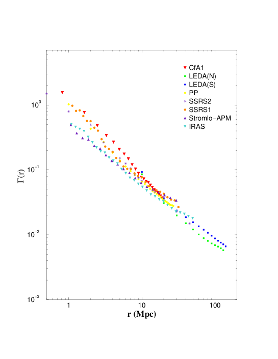
Figure 1: Full correlation analysis for the various available redshift surveys in the range of distance $0.5\div 1050h^{-1}Mpc$. The slope is $-1$, which corresponds to fractal dimension $D=2$. (From Sylos Labini et al., 1998).

5 Problems of the Standard FRW scenario

In his classic paper, Hubble$\!{}^{{\bf?}}$ found a roughly linear relation between the spectral line displacement $z=(\lambda_{obs}-\lambda_{em})/\lambda_{em}$ of the line emitted by a far away galaxy $\lambda_{em}$, and its distance $r$. The empirical Hubble Law may be written as

$$cz=H_{0}r\;,$$ (3)

where $c$ is the velocity of light and $H_{0}$ is the Hubble constant. As an observationally established relation, the Hubble law does not refer to any interpretation of redshift. Space expansion and Doppler mechanisms in falt space for redshift, yields at first order to Eq.3. If redshift is interpreted as a motion effect, then

$$V\approx H_{0}r$$ (4)

where $V$ is either space expansion velocity $v_{exp}$ or ordinary velocity of a body moving in the Euclidean space. Usually this velocity-distance relation is called the Hubble Law, but it is more correct to regard it as the redshift-distance relation of Eq.3. This is based on the primarily measured quantities (redshift and distance), while velocity is inferred from redshift in the frame of some cosmological model.

Since its discovery, the validity of the Hubble law has been confirmed in an ever increasing distance interval where local and more remote distance indicators may be tied together. Recently, several new distances have been measured to local galaxies using observations of Cepheid variable stars, thanks to the Hubble Space Telescope programmes$\!{}^{{\bf?}}$. Along with previous Earth-based Cepheid distances, methods like Supernovae Ia and Tully-Fisher have been better calibrated than before and confirm the linearity with good accuracy up to $z\approx 0.1$. Brightest cluster galaxies trace the Hubble law even deeper, up to $z\approx 1$, and radio galaxies have provided such evidence at still larger redshifts$\!{}^{{\bf?}}$.

It is well known that there are small deviations $\delta V$ from the Hubble velocity $V_{H}$, connected with local mass concentrations such as the Virgo Cluster, and, possibly the Great Attractor. However, these perturbations are still only of the order $\delta V/V_{H}\sim 0.1$, while in the general field the Hubble law has been suggested to be quite smooth, with $\delta V$ around $50km/s$$\!{}^{{\bf?}}$.

Without the actual knowledge of matter distribution, the linearity and the small scatter of the observed Hubble law for field galaxies would make one guess that the galaxies are uniformly distributed: as it was asserted above, this is the basis for the linear Hubble law in the standard cosmology. In fact, it has been a common supposition that when the Hubble law was found in the nearby space, one finally had entered a cosmologically representative region of the Universe. At the same time, it has been clear that at small distances where Hubble found his relation, the galaxy distribution is quite inhomogeneous. Though, it has been believed that beyond some, not too large distance, the distribution should become uniform.

As we have already mentioned, studies of the 3-dimensional galaxy universe have shown that de Vaucouleurs’ prescient view on the matter distribution is valid at least in the range of scales $\sim 0.5\div 200\;Mpc$ (hereafter $H_{0}=55km/sec/Mpc$). The Hubble and de Vaucouleurs laws describe very different aspects of the Universe, but both have in common universality and observer independence. This makes them fundamental cosmological laws and it is important to investigate the consequences of their coexistence at similar length-scales. In Fig.2 we display these laws together.

Figure 2: Hubble redshift-distance and de Vaucouleurs density-distance laws in the distance scales from $1$ to $500Mpc$ ($H_{0}=55km/s/Mpc$). The Hubble law (increasing from left to right) is constructed from: galaxies with Cepheid-distances for $cz>0$ (triangles), galaxies with Tully-Fisher (B-magnitude) distances (stars), galaxies with SNIa-distances for $cz>3000km/s$ (filled circles). TF-distance points are generally averages of a few tens of galaxies from the ”unbiased plateau” of the method of normalized distances. Redshift $cz$ is reduced to the Local Group center and contains the small correction due to the Virgo infall velocity field. The solid line corresponds to the Hubble law with $H_{o}=55km/s/Mpc$. The de Vaucouleurs law (decreasing from left to right) in the normalized form is constructed from the computation of the conditional average density in the following redshift surveys: CfA1 (crosses), Perseus-Pisces, LCRS (filled diamonds), ESP (triangles left) and LEDA (Sylos Labini et al., 1998). The normalization between the different densities takes into account the different magnitude limited of the various redshift surveys. The dotted line corresponds to the de Vaucouleurs law with correlation exponent $\gamma=1$, i.e. $D=2$. (From Baryshev et al., 1998)

A representative Hubble law has been taken from Fig.4 of Teerikorpi (1997)$\!{}^{{\bf?}}$, based on Cepheid distances to local galaxies, Tully-Fisher distances from the KLUN programme, and Supernovae Ia distances. The behavior of the conditional density (De Vaucouleurs law) presented in Fig.2 has been taken from Sylos Labini et al.(1998).

The puzzling conclusion from Fig.2 is that the strictly linear redshift-distance relation is observed deep inside the fractal structure. (Note that in the analysis of galaxy redshift surveys one uses the Hubble law for the distance determinations as an experimental fact, i.e. any assumption has been used). This empirical fact presents a profound challenge to the standard model where the homogeneity is the basic explanation of the Hubble law, and ”the connection between homogeneity and Hubble’s law was the first success of the expanding world model” $\!{}^{{\bf?}}$. This also reminds us the natural reaction of several authors: ”In fact, we would not expect any neat relation of proportionality between velocity and distance [for such close galaxies]” $\!{}^{{\bf?}}$.

However, contrary to the expectations, modern data show a good linear Hubble law even for nearby galaxies. How unexpected this actually is, can be expressed quantitatively for the standard model and is briefly discussed below (for a more detailed discussion see Baryshev et al., 1998).

According to the standard Big Bang model the universe obeys Einstein’s Cosmological Principle: it is homogeneous, isotropic and expanding $\!{}^{{\bf?}}$$\!{}^{{\bf?}}$. Homogeneity of matter distribution is the central hypothesis of the standard cosmology because it allows one to introduce the space of uniform curvature in the form of the Robertson-Walker line element $R(t)$. This line element leads immediately to a linear relation between velocity and proper distance. Indeed, consider a comoving body at a fixed coordinate distance from a comoving observer. At cosmic $t$, let $l=R(t)y$ be the proper distance from the observer. The expansion velocity $v_{exp}=dl/dt$, defined as the rate of change of the proper distance $l$, is

$$v_{exp}=Hl=c\cdot\frac{l}{l_{H}}$$ (5)

where $H=\dot{R}/R$ is the Hubble constant and $l_{H}=c/H$ is the Hubble distance. In this way, the linear velocity-distance relation of Eq.5 is an exact formula for all Friedmann models and a rigorous consequence of spatial homogeneity. In particular, for $l>l_{H}$, the expansion velocity $v_{exp}>c$. Such an apparent violation of special relativity is consistent with general relativity $\!{}^{{\bf?}}$.

In the expanding space the wavelength of an emitted photon is progressively stretched, so that the observed redshift $z$ is given by Lemaitre’s redshift law

$$z=\frac{R(t_{obs})}{R(t_{em})}-1$$ (6)

which is a consequence of the radial null-geodesic of the FRW line element. For $z\ll 1$ Eq.6 yields $z\approx dR/R\approx H_{0}dt\approx l/l_{H}$, and from Eq.5 one gets the approximate velocity-redshift relation that is valid for small redshifts

$$v_{exp}\approx cz\;.$$ (7)

We note that the expansion velocity-redshift relation differs from the relativistic Doppler effect. So, the space expansion redshift mechanism in the standard model is quite distinct from the usual Doppler mechanism. We stress this points, because in the literature these two redshift mechanisms are often confused. In the context of the standard cosmology, it has been natural to interpret the Hubble Law as a reflection of Eq.7 and to regard the coefficient of proportionality $H_{0}$ in Eq.3 as the present value of the theoretical Hubble constant $H$ from Eq.5.

We consider now the case of an expanding universe, where an average density is well defined and has a constant value $\rho_{0}$. In such a case, by neglecting relativistic effects and the terms depending on pressure, according to the linear approximation, there is a velocity deflection $\delta V$ from the unperturbed Hubble flow $V_{H}=H_{o}r$ in the scale where the density perturbation is $\delta\rho$. In the case of zero cosmological constant and spherical mass distribution, this deflection has grown during the Hubble time to the present value which is (Eq.20.55 from Peebles, 1993):

$$\frac{\delta V}{V_{H}}=\frac{1}{3}{\Omega_{0}}^{0.6}\frac{\delta\rho}{\rho_{0}}$$ (8)

where $\Omega_{0}=\rho_{0}/\rho_{crit}$ is the density parameter of the Friedmann model. This approximation holds in the limit $\delta\rho/\rho_{0}\ll 1$.

Let us consider a two-component model for the density distribution in a Friedmann universe. First, there is the component which exhibits fractal behavior up to a maximum scale, and which we call $\lambda_{0}$. At larger scales this component is homogeneous with an average density $\rho_{lum}$. The second component is dark matter, homogenous at all scales, with density $\rho_{dark}$ (see fig.3).

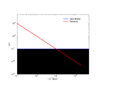
Figure 3: A simple two-component model: galaxies have a fractal distribution corresponding to correlated density fluctuations superimposed to a uniform background. In the figure it is shown the behaviour of the number density of galaxies and the matter density (from Durrer & Sylos Labini 1998)

For such a model there is a definite constant density at all scales larger than $\lambda_{0}$. This density $\rho_{0}$ is the sum of $\rho_{lum}$ and $\rho_{dark}$. This means that the behavior of this model at scales larger than $\lambda_{0}$ is identical to that of the Friedmann model for which

$$\Omega_{0}=\Omega_{dark}+\Omega_{lum}\;.$$ (9)

At such large scales the Hubble law is unperturbed. The density distribution of luminous matter for scales $r<\lambda_{0}$, can be written as

$$\rho_{lum}(r)=\rho_{lum}\left(\frac{\lambda_{0}}{r}\right)^{\gamma}$$ (10)

where $\gamma=3-D$ as usual. For the scales $r\geq\lambda_{0}$ we have that

$$\rho_{lum}(r)=\rho_{lum}=\rho_{lum}(\lambda_{0})\;.$$ (11)

The density contrast can be written as

$$\frac{\delta\rho}{\rho_{0}}=\frac{\rho_{lum}(r)+\rho_{dark}-\rho_{0}}{\rho_{0}}$$ (12)

In terms of the Friedmann density parameters as defined above, this becomes, at scales smaller than $\lambda_{0}$:

$$\frac{\delta\rho}{\rho_{0}}=\frac{\Omega_{lum}}{\Omega_{0}}\left(\left(\frac{r}{\lambda_{0}}\right)^{-\gamma}-1\right)\;.$$ (13)

At scales larger than $\lambda_{0}$ the density contrast clearly vanishes.

By using the linear approximation (Eq.8), we may obtain a rough estimation of the expected deflection from the Hubble law in the two component model, for the scale in which the density contrast is less than 1. Although the linear approximation is valid only for $\delta\rho/\rho_{0}\mathrel{\hbox to0.0pt{\lower 3.0pt\hbox{$\mathchar 536\relax$}\hss}\raise 2.0pt\hbox{$\mathchar 316\relax$}}1$, the obtained results give a first quantitative indication of the effects of self-similar fluctuations. Moreover the assumption of spherical mass distribution is a rough one, and it holds only for average quantities. In the case of real fractals deviation from spherical symmetry can play an important role, at least at small scale. Under these approximations, the radial velocity measured by an average observer at scale $r<\lambda_{0}$ is (from Eq.8)

$$V_{obs}=V_{H}\left(1-\left(\frac{1}{3}\right){\Omega_{0}}^{-0.4}\Omega_{lum}\left(\left(\frac{r}{\lambda_{0}}\right)^{-\gamma}-1\right)\right)$$ (14)

Actually, this is the prediction averaged over many observers in different fractal structure points (galaxies). For any particular observer, there will be a deflection from this average law.

We take the maximum scale $\lambda_{0}$ of fractality and the fractal dimension $D$ from the observed cosmological de Vaucouleurs Law and calculate the expected deflections from the Hubble law in our two-components Friedmann model. In Fig.4

Figure 4: We show three theoretical predictions for the velocity deflection in the case where the observed fractal structure contains all the matter, i.e. when $\Omega_{lum}=\Omega_{0}$. We have fixed $\lambda_{0}=200Mpc$ and fractal dimension $D=2$. The predictions correspond to three values of the cosmological density parameter $\Omega_{0}=1,0.1,0.01$. (From Baryshev et al., 1998)

we show three theoretical predictions for the velocity deflection in the case where the observed fractal structure contains all the matter, i.e. when $\Omega_{lum}=\Omega_{0}$. We have fixed $\lambda_{0}=200Mpc$ and fractal dimension $D=2$. In this case the linear approximation holds for $r\mathrel{\hbox to0.0pt{\lower 3.0pt\hbox{$\mathchar 536\relax$}\hss}\raise 2.0pt\hbox{$\mathchar 318\relax$}}130Mpc$. At smaller scales we should consider non-linear effects which are not simple to be treated. However we should expect even stronger velocity perturbations, due to the highly inhomogeneous structures distribution. The predictions correspond to three values of the cosmological density parameter $\Omega_{0}=1,0.1,0.01$. From Fig.4 it follows that such Friedmann models, purely fractal within $200Mpc$, are excluded if $\Omega_{0}\mathrel{\hbox to0.0pt{\lower 3.0pt\hbox{$\mathchar 536\relax$}\hss}\raise 2.0pt\hbox{$\mathchar 318\relax$}}0.01$. This confirms the previous suggestions that small $\Omega_{0}$ is needed for hierarchic models (Sandage, et al.1972 - hereafter STH).

For instance, there is one possible way to save the Friedmann universe with the critical density parameter $\Omega_{0}=1$. It was implied already by STH that dark matter, uniformly filling the whole universe and decreasing the relative density fluctuations, could reconcile the observed fractal structure with the linear Hubble law. However, they did not give a quantitative estimate of the amount of dark matter needed. With the new data on the Hubble and de Vaucouleurs laws, we can derive the lower limit for the amount of the needed uniform dark matter. In Eq.14 we fix $\Omega_{0}=1$ and let $\Omega_{lum}$ have different values. Fig.5

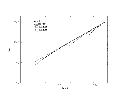
Figure 5: In this case the total density is $\Omega_{0}=1$. We show the behaviour of $V_{obs}$ derived by the linear perturbation approximation in the case $\delta\rho/\rho_{0}\ll 1$, for various values of $\Omega_{lum}$. The fractal dimension of luminous matter is $D=$ up to $\lambda_{0}=200Mpc$. (From Baryshev et al., 1998)

gives the developed version of the STH test, now showing that $\Omega_{dark}$ should be larger than 0.99. If the actual maximum scale of fractality is larger than $200Mpc$ (with $D=2$), then the amount of luminous matter may be in conflict with the Big Bang nucleosynthesis prediction for baryonic matter. For example, if $\lambda_{0}\mathrel{\hbox to0.0pt{\lower 3.0pt\hbox{$\mathchar 536\relax$}\hss}\raise 2.0pt\hbox{$\mathchar 318\relax$}}1000Mpc$ (as suggested by Sylos Labini et al., 1998) then $\Omega_{lum}$ will be probably less than 0.001.

It should be emphasized that this estimate of the amount of dark matter is independent on the physics of the early universe. It also does not depend on the determination of mass-to-luminosity ratio of galaxies.

6 Inconsistency of CDM models

It is simple to see that a fractal behavior of galaxy distribution with dimension $D\approx 2$ up to, at least, $\sim 50h^{-1}Mpc$ is not compatible with standard CDM models. In fig.6

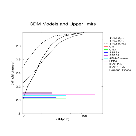
Figure 6: The fractal dimension versus distance in three Cold Dark Matter models of power spectra with shape and normalized parameters as reported in the labels (solid lines) (from Wu et al., 1998). We show also the different experimental determinations of the fractal dimension we have obtained. No agreement can be found at any scale.

we show the behavior of the fractal dimension versus distance in three Cold Dark Matter models of power spectra with shape and normalized parameters (from Wu et al., 1998). We may see that a fractal dimension of $D\approx 2$ at $\sim 40\div 50h^{-1}Mpc$ is incompatible with all the models. Probably by varying the parameters of the simulation (or the mixture of Hot and Cold Dark Matter) one may hope to obtain a better agreement. Any new survey has required a new adjustment of the parameters and this alone shows the internal problems of the standard models of galaxy formation.

We belive that the most important theoretical consequence of our results is that one may shift the attention of the study from correlation amplitudes to correlation exponents (Sylos Labini et al.1998, and Durrer & Sylos Labini, 1998).

7 Discussion

Investigation of the large scale distribution of galaxies in the universe is now in a new phase, which is characterized by new observational data and new methods of analysis. It has become an especially hot and debated topic in cosmology, because the revealed fractality contradicts Cosmological Principle in the sense of homogeneity but not in the sense of the equivalence of all the observers$\!{}^{{\bf?}}$. Above we have discussed the fractality and its implications for cosmology. Our main conclusions are:

• Observations show that there is a fractal distribution of galaxies, having fractal dimension $D\approx 2$ in the scale range from $1Mpch^{-1}Mpc$ to, at least, $100h^{-1}Mpc$. While there is a general agreement on the small scale fractal properties of galaxy distribution, the actual value of $D$ and the eventual presence of an upper cut-off, are still matter of debate$\!{}^{{\bf?}}$ $\!{}^{{\bf?}}$. (See the web page http://www.phys.uniroma1.it/DOCS/PIL/pil.html where all these materials have been collected).

• The traditional statistical analysis based on the assumption of homogeneity (i.e. $\xi(r)$), should be replaced by the more general methods of modern statistical physics. Such methods are able to characterize scale-invariant distributions as well as regular ones.

• An isotropic fractal distribution is fully compatible with the reasonable requirement of the equivalence of all the observers. Hence the Standard Cosmological Principle, which requires isotropy and homogeneity, may be replaced by the Conditional Cosmological Principle. In such a case the condition of local isotropy around any structure point, without the assumption of analyticity of matter distribution, does not imply the homogeneity of matter distribution.

• The paradox of linear Hubble law within the fractal de Vaucouleurs density-distance law is sharpened with the new data: strong deflections from the Hubble flow are expected in the framework of the standard Friedmann model.

• From a developed version of the old Sandage-Tammann-Hardy test we derive the minimum amount of the uniform dark matter, $\Omega_{dark}=0.99$, which is consistent with the presently known Hubble and de Vaucouleurs laws. This result is independent of the early universe physics. If the maximum scale of fractality is larger than $100h^{-1}Mpc$, this test may be regarded as crucial for the standard cosmology.

• We have shown that a fractal behavior of galaxy distribution with dimension $D\approx 2$ up to, at least, $\sim 50h^{-1}Mpc$ is not compatible with standard CDM models.

• One the most important theoretical consequence of our results is that one may shift the attention of the study from correlation amplitudes to correlation exponents. The revision of the concept of bias (Durrer & Sylos Labini, 1998) is an example of such a situation. De Vega et al.$\!{}^{{\bf?}}$ $\!{}^{{\bf?}}$ have proposed a field theory approach to the fractal structure of the universe. In such a model the dominant dynamical mechanism responsible for the scale invariant distribution is self-gravity itself. This model represents an interesting approach on the lines of modern statistical physics previously: it focuses on the expoenents rather than to the amplitudes of correlation. In the near future we are planning to study some experimental consequences of such a theoretical framework.

References

- [1] de Vaucouleurs, G., Science, 167, 1203-1213 (1970
- [2] Mandelbrot, B.B., Fractals:Form, Chance and Dimension, W.H.Freedman, (1977)
- [3] Peebles, P.E.J., 1980 ”The Large Scale Structure of The Universe” (Princeton Univ.Press.);
- [4] Peebles, P.E.J., 1993 Principles of Physical Cosmology, Princeton Univ.Press, (1993)
- [5] Peebles, P.E.J., 1998 In the Proceed. of the Conference ”les Rencontres de Physique de la Vallee d Aosta” (1998) ed. M. Greco (astro-ph/9806201)
- [6] Pietronero L., 1987 Physica A, 144, 257
- [7] Sylos Labini, F., Montuori, M.and Pietronero,L. 1997, Physics Report 293, 61-226 (1998)
- [8] Mandelbrot B., in the Proc. of the Erice Chalonge School Eds. N. Sanchez and H. de Vega, World Scientific (1998)
- [9] Coleman, P.H. and Pietronero, L.,1992 Phys.Rep. 231,311
- [10] Sylos Labini, F. et al., In preparation (1998)
- [11] Joyce M., Sylos Labini F., Montuori M. and Pietronero L. Astronom.Astrophys. 1998 Submitted (astro-ph/9805126)
- [12] Hubble, E., Proc.Nat.A.Sci., 15, 168-173 (1929)
- [13] Tammann, G.A., et al.in Science with the Hubble Space Telescope - II, 9-19, Space Telescope Science Institute, Eds. Benvenuti et al.(1996)
- [14] Sandage, A., in The Deep Universe, eds. Binggeli, B., Buser, R., Springer, (1995)
- [15] Baryshev Y. V., Sylos Labini F., Montuori M., Pietronero L. and Teerikorpi, P. Fractals , in press (1998).
- [16] Teerikorpi, P., Ann.Rev.Astron.Astrophys 35, 101-136 (1997)
- [17] Peebles, P.J.E., et al.Nature, 352, 769-776 (1991)
- [18] Weinberg, S., The First Three Minutes, p.26, Basic Books, New York (1977)
- [19] Weinberg, S., Gravitation and Cosmology, John Wiley & Sons (1972)
- [20] Harrison, E., Astrophys.J., 403, 28-31 (1993)
- [21] Durrer R. and Sylos Labini F. (1998) Preprint (astro-ph/9804171)
- [22] Sandage, A,. et al.Astrophys.J. 172, 253-263 (1972)
- [23] Wu K.K.S., Lahav O. and Rees M., (1998) Nature submitted (astro-ph/9804062)
- [24] Teerikorpi, P., et al.Astron.Astrophys. In The Press (1998); astro-ph/9801197
- [25] de Vega H., Sanchez N. and Combes F., (1996) Nature 383, 53
- [26] de Vega H., Sanchez N. and Combes F. (1998) , Ap. J In Press