Abstract

The local H i mass function (HiMF), like the optical luminosity function, is an important observational input into models of cosmology and galaxy evolution. It is a helpful framework for assessing the number density of gas rich dwarf galaxies, which are easily missed in optically selected galaxy samples, as well as for determining the cosmological density of neutral gas at the present epoch. For H i masses larger than $10^{8}~{}\mbox{${\rm M}_{\odot}$}$ the HiMF is determined with reasonable accuracy and the same function is obtained from both optical and H i selected samples of galaxies. However, the faint tail below $\mbox{$M_{\rm HI}$}<10^{7}~{}\mbox{${\rm M}_{\odot}$}$ is still ill-constrained and leaves room for a population of gas rich dwarfs or free floating H i clouds which hypothetically could contribute significantly to the local gas density. Determining the faint tail far below H i masses of $10^{7}~{}\mbox{${\rm M}_{\odot}$}$ will be a great challenge for the future.

THE LOCAL H i MASS FUNCTION

Kapteyn Astronomical Institute, Groningen, The Netherlands

1 Introduction

The H i mass function (HiMF), the H i equivalent to the better known optical luminosity function (LF) defines the number of galaxies per cubic Mpc as a function of H i mass $M_{\rm HI}$. This function is an important constraint in theories of cosmology and galaxy evolution. The shape of the local HiMF tells us how the neutral gas in the nearby Universe is distributed over galaxies of different masses. For example, semi-analytical models of galaxy formation require detailed measurements of the HiMF and the LF to test the predictions (e.g., [34]). In contrast to the LF, the HiMF should also constrain the number density of gas rich dwarfs and low surface brightness (LSB) galaxies. It has been shown that these objects are easily missed in optical surveys which are used to evaluate the LF [8, 24], but they could contribute a significant part of the HiMF. Also the often speculated upon, but yet unidentified class of free floating H i clouds are definitively missed in LFs but are hypothetical contributors to the HiMF.

Besides the shape of the HiMF, also the normalization is of great importance to cosmology. The integral over the function yields the cosmological neutral gas density of the local Universe. This measurement anchors the estimates of the neutral gas densities at higher redshift determined from damped Ly$\alpha$ systems, seen in absorption in the spectra of background quasars. These systems are generally considered to be the high $z$ equivalents of the cold gas disks of present day spiral galaxies. The exact measurement of the gas density as a function of redshift brackets theories of structure formation and also helps in the understanding of the physical processes of gas cooling and star formation. An important question is whether the LSB galaxies and the gas rich dwarfs make a significant addition to the cosmological neutral gas density at the present epoch.

2 How To Measure an HiMF

Different methods can be employed for evaluating an HiMF. The largest variety lies in the sample of galaxies that is used to derive the function. Basically two classes of galaxy samples can be distinguished: optically selected galaxy samples and H i selected galaxy samples. This section briefly describes both methods.

2.1 HiMF Based on Optically Selected Galaxies

An HiMF can easily be derived from optical luminosity functions when a conversion factor from optical luminosity to H i mass is used. Suppose the LF can be described by a Schechter function of the form

$$\phi(L)dL=\mbox{$\phi^{*}$}\left(\frac{L}{L^{*}}\right)^{\alpha}\exp-\left(\frac{L}{L^{*}}\right)d\left(\frac{L}{L^{*}}\right),$$ (1)

where $L^{*}$ is the characteristic luminosity that defines the knee in the LF, $\phi^{*}$ is the normalization, and $\alpha$ is the value that defines the slope of the faint end. By using a relation between optical magnitude $M$ and H i mass, for example $\log\mbox{$M_{\rm HI}$}=A-BM,$ an HiMF can be derived:

$$\Theta(\mbox{$M_{\rm HI}$})d(\mbox{$M_{\rm HI}$})=\frac{0.4}{B}\,\mbox{$\phi^{*}$}\left(\frac{\mbox{$M_{\rm HI}$}}{\mbox{$M^{*}_{\rm HI}$}}\right)^{(\alpha+1)\frac{0.4}{B}-1}\exp-\left(\frac{\mbox{$M_{\rm HI}$}}{\mbox{$M^{*}_{\rm HI}$}}\right)^{\frac{0.4}{B}}d\left(\frac{\mbox{$M_{\rm HI}$}}{\mbox{$M^{*}_{\rm HI}$}}\right).$$ (2)

The low-mass slope of the HiMF is related to the faint-end slope of the LF as $\alpha_{\rm HI}=(\alpha_{\rm opt}+1)\frac{0.4}{B}-1$. Rao & Briggs [27] applied this method by using different LFs and conversion factors for different morphological types and added up the results to obtain a global $M_{\rm HI}$ distribution function. The HiMF that they derived is well-fit by a Schechter function with $\alpha\approx-1.1$. Intuitively one would believe that a trend of increasing H i richness for low luminosity galaxies ($B<0.4$) implies a steep low mass end of the mass function. However, Rao & Briggs already stressed that for realistic values of $B$ ($\sim 0.35$ [10]), $\alpha_{\rm HI}\approx\alpha_{\rm opt}$, especially for $\alpha_{\rm opt}$ in the range $-1.0$ to $-1.3$.

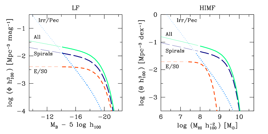
Figure 1: Left panel: Luminosity function for various morphological types taken from Marzke et al. [23]. Right panel: converted H i mass function following the procedure described in the text.

In Fig. 1 an example of this method is shown. The luminosity function for various morphological types taken from Marzke et al. [23] is shown in the left panel. The right panel shows the derived H i mass functions, using different values of $A$ and $B$ for the different morphologies. It is clear that the HiMF is dominated by spiral galaxies, although at the very low mass end the irregulars seem to overtake the number densities. However, this dominance occurs at luminosities below $M_{B}=-14$, the magnitude limit of the Marzke et al. sample.

A slightly modified form of this method of finding an HiMF for optically selected galaxies is to use the measured H i fluxes for a sample of galaxies with well-understood selection criteria. For example, Hoffman et al. [16] conducted a series of pointed observations with the Arecibo telescope of known galaxies in the Virgo cluster. They constructed a preliminary HiMF and concluded that there is no excess of gas rich dwarf galaxies. Briggs & Rao [4] reanalyzed these data supplemented with the Tully & Fisher catalog of H i observations of spiral galaxies, and were able to construct the HiMF over the range $10^{7}$ to $10^{10}~{}\mbox{${\rm M}_{\odot}$}$. They also concluded that there is no evidence for a sharp rise in the number of gas rich dwarf galaxies, and that in clusters the HiMF might even go down.

Although the estimation of the space density of gas rich objects using galaxies that are selected on their star light is very instructive, it does not yield an unbiased HiMF for all gas containing objects. The HiMF determined by optically selected galaxies defines a lower limit to the “real” HiMF, and it is not inconceivable that large populations of extragalactic objects are missing from the analysis. It has become clear of late that low surface brightness (LSB) galaxies contribute significantly to the number density of galaxies in the local Universe (e.g., [37, 5]). Since these galaxies are found to be rich in HI [32] they are likely candidates to make a contribution to the HiMF, while they are easily missed in optical surveys [8]. Objects that are most certainly missed in surveys in optical wavelengths are hypothetical free floating H i clouds. A conversion from a LF to a HiMF would never include these objects.

2.2 HiMF Based on H i Selected Galaxies

The most ideal method to measure an HiMF is to use a “blind” survey in H i. No biases against galaxies’ surface brightnesses or magnitudes are introduced that way. The HiMF can be constructed directly and suffers no bias against LSB galaxies, gas rich dwarfs or even free floating H i clouds. The major problem is that finding a galaxy in H i is much more difficult than finding it optically. Blind surveys in H i take hundreds of hours of observing time to yield only few dozen galaxies, while optical surveys systematically produce catalogs of thousands of galaxies. For illustration, the first published blind H i survey in the field (Shostak [33]) took many days of observing time with the NRAO 300 ft telescope and yielded only one detection which later turned out to be a high velocity cloud gravitationally bound to the Milky Way galaxy. In order to increase the detection efficiency many surveys were pointed toward known overdensities: groups and clusters of galaxies. The M81, Sculptor, CVn I and NGC 1023 groups [12, 20, 11] as well as the the Hydra [25], Hercules [7], Centaurus and Fornax [1] clusters have been surveys extensively in the 21cm line. The conclusion that can be drawn from these surveys are 1) the shape of the HiMF is similar to that that is derived in the field from optically selected galaxies, 2) no excess of gas rich dwarfs has been found, and 3) no H i clouds without stars are found. Also global underdensities (voids) have been surveyed [39, 18], but no H i selected galaxies have been found there.

A fair comparison of the HiMF for H i selected galaxies with that from optically selected galaxies requires a blind H i survey of the field, with no preference to known over- or underdensities. Henning [13, 14] conducted a series of pointings on lines of constant declination over a redshift range of 7200 km/s. A total number of 39 significant detections were recorded, of which 50% were previously unknown. While Hennings HiMF seems to be indicative of an increasing number of dwarf galaxies, the overall function lies below the lower limit to the HiMF set by counting the optically selected population.

Two large surveys in the 21cm line have been conducted recently, both with the Arecibo telescope. The results from one of these surveys, named AHiSS (Arecibo H i Strip Survey) is the topic of the next section. The other survey, similar in size, is discussed in Spitzak [36] and Schneider [31]. There are currently surveys in progress at Dwingeloo [15], at Arecibo (The Dual-Beam Survey [31]), and at Parkes [17]. The latter will cover the whole southern sky out to 12,700 km/s.

3 The Arecibo H i Strip Survey

The survey was carried out during the period of August 1993 until February 1994 when the Arecibo telescope was being upgraded. Since the pointing was immobilized, the data were taken in drift-scan mode. Two strips of constant declination ($\delta=14^{\circ}$ and $\delta=23^{\circ}$) were traced, together covering 17 hours of RA. The total sky coverage, including the side lobes, was 65 square degrees, wile the survey depth was $cz=7400~{}\mbox{$\rm km\,s^{-1}$}$. The minimal detectable H i mass at the full depth of the survey was $1.5\times 10^{8}~{}h_{100}^{-2}~{}\mbox{${\rm M}_{\odot}$}$ in the main beam, while $6\times 10^{5}~{}h_{100}^{-2}~{}\mbox{${\rm M}_{\odot}$}$ of H i could be detected at $7~{}h_{100}^{-1}~{}\rm Mpc$.

A total of 66 significant ($5\sigma$) detections were found, of which 32 are listed in existing catalogs of optically selected galaxies. All detections that are sufficiently far away from the Galactic equator ($b>10^{\circ}$) to avoid severe extinction by Galactic dust were imaged in the $B$-band with the 2.5 Isaac Newton Telescope on La Palma. All H i signals were identified in the optical images, and were found to be ordinary galaxies, having both stars and gas. No free floating H i clouds were detected in this survey, which puts serious constraints on the existence of these objects which are potentially a population of protogalaxies.

21cm follow-up with the VLA in D-configuration was performed on all significant detections. These observations were required to determine more accurate fluxes and positions for all sources. Another important reason for doing follow-up with higher angular resolution, is to see whether the signals were caused by single clouds or galaxies, or by pairs or small groups, whose line emission might stack up in the same channels. We found that this latter situation to occurs in five of the 61 cases. For surveys which make use of dishes smaller than the Arecibo telescope, and therefore scan the sky with larger beam sizes, this effect is probably more important. Higher resolution 21cm follow-up is therefore essential to accurately determine the number of galaxies in the survey, their H i masses and to make adequate identifications with optical images.

From a comparison of the H i and optical properties between the cataloged and uncataloged galaxies in our H i selected sample we conclude that the uncataloged galaxies are preferentially the ones with lower average optical surface brightness, lower luminosity, lower H i mass, smaller linear sizes and higher gas to light ratios [44]. However, this does not imply that a blind H i survey yields a population of galaxies that has previously gone unnoticed in optical galaxy surveys. Simply because in these two strips the sky has been surveyed deeper in H i than in the optical, the uncataloged galaxies will mostly be dwarf galaxies or galaxies with lower optical surface brightness. Furthermore, the restricted bandwidth of the receiving system imposes a strict limit on the maximum redshift of the detected galaxies, this limits does not exist in optical surveys. These two effects cause a predominance of low luminosity systems in an H i selected galaxy sample. It is well established that decreasing luminosity and decreasing surface brightness correlate well with increasing $M_{\rm HI}/L$ ratio [41, 6]. Therefore, the differences found between cataloged and uncataloged galaxies are a natural result of the survey technique and do not imply that the new H i selected galaxies have properties that set them apart from known, optically selected galaxies.

A HiMF for this sample of H i selected galaxies is determined by using the $1/{\cal V}_{\rm max}$ method [30]. This method consists of summing the reciprocals of the volumes corresponding to the maximum distance at which each object could be placed and still remain within the sample. Advantages of this method are that the HiMF is automatically normalized and that it is nonparametric, that is it does not use a Schechter function as an intrinsic assumption about the shape of the HiMF. A recent overview of the different galaxy luminosity function estimators is given by Willmer [42], who tests the validity of different methods by means of Monte-Carlo simulations. Careful examination of his tables shows that the $1/{\cal V}_{\rm max}$ method (with binning in magnitudes) recovers the input luminosity function satisfactorily, and equally well as the more conventional parameterized maximum likelihood method [29] or the stepwise maximum likelihood method (SWLM [9]).

Fig. 2 shows the HiMF for the AHiSS. The solid points show the HiMF per half decade, normalized such that they represent the number of galaxies per $\rm Mpc^{3}$ per decade. Errorbars represent $1\sigma$ errors from Poisson statistics. The solid line indicates a best fit Schechter function to the points, parameterized by

$$\Theta(\mbox{$M_{\rm HI}$})d\mbox{$M_{\rm HI}$}=\theta^{*}\left(\frac{\mbox{$M_{\rm HI}$}}{\mbox{$M^{*}_{\rm HI}$}}\right)^{\alpha}\exp-\left(\frac{\mbox{$M_{\rm HI}$}}{\mbox{$M^{*}_{\rm HI}$}}\right)d\left(\frac{\mbox{$M_{\rm HI}$}}{\mbox{$M^{*}_{\rm HI}$}}\right),$$ (3)

where $\alpha$ is the slope of the faint tail, $\theta^{*}$ is the normalization, and $M^{*}_{\rm HI}$ is the characteristic mass that defines the knee in the HiMF. Because there are no H i masses lower than $10^{7}$ or higher than $10^{10}~{}\mbox{${\rm M}_{\odot}$}$ detected by the AHiSS, the HiMF is almost unconstrained in these regions. However, upper limits to the space density of H i rich galaxies or H i clouds can be determined by showing the sensitivity function in the same figure. The sensitivity function is defined by $\phi=1/{\cal V}$, where ${\cal V}$ is the effective search volume. The arrows indicate upper-limits to the HiMF, on the left they follow this sensitivity function, on the right they are determined by a complementary survey with Arecibo over the redshift range $cz=$ 19,000 to 28,000 $\rm km\,s^{-1}$. The best fit parameters of the Schechter function are $\alpha=-1.20$, $\theta^{*}=0.014~{}\rm Mpc^{-3}$ and $\log(\mbox{$M^{*}_{\rm HI}$}/\mbox{${\rm M}_{\odot}$})=9.55$.

Figure 2: H i mass function from the Arecibo H i Strip Survey. The thin line is the sensitivity of the survey defined by $\phi=1/{\cal V}$, where $\cal V$ is the effective search volume. In the region $10^{7}{\rm M}_{\odot}<M_{\rm HI}<10^{10}{\rm M}_{\odot}$ this function defines an upper limit to the space density of intergalactic H i clouds without stars. The measured H i mass function per decade is shown by the points. The thick line is a Schechter luminosity function with parameters as given in the upper right corner. The arrows show upper limits to the space density of H i rich galaxies or intergalactic H i clouds. The two arrows on the right are from a complementary survey with the Arecibo telescope over the range 19,000 to 28,000 ${\rm km\,s}^{-1}$.

3.1 The integral H i density

As was mentioned in section 1, the local HiMF can be used to determine the integral gas density, $\Omega_{\rm g}$, at $z=0$. At high redshifts $\Omega_{\rm g}$ can be derived from the study of damped Ly$\alpha$ systems, high column density gas clouds seen in absorption in the spectra of background quasars. At low redshifts, these measurements are hampered by poor statistics for several reasons: due to the expansion of the Universe the expected number of absorbers decreases with decreasing redshift, the Ly$\alpha$ line is not observable from the ground for redshifts smaller than 1.65, and starlight and dust in the absorbing foreground galaxies hinder the identification of the background quasars. The most recent determinations of the gas density from damped Ly$\alpha$ systems show that the redshift range from 0 to 1.65, which corresponds to more than three quarters of the age of the Universe ($q_{0}=0.5$), is covered by only about 20 systems [40]. Furthermore, the lowest redshift damped Ly$\alpha$ system currently known is at $z=0.09$ [28], illustrating that a $z=0$ point can not yet reliably be derived from damped Ly$\alpha$ observations.

The gas density detected in the AHiSS can be readily determined by taking the integral over the HiMF multiplied by $M_{\rm HI}$. This yields $\mbox{$\rho_{\rm HI}$}=\Gamma(2+\alpha)\theta^{*}\mbox{$M^{*}_{\rm HI}$}$, where $\rho_{\rm HI}$ is the neutral gas density in $\mbox{${\rm M}_{\odot}$}/\rm Mpc^{3}$. Using the values from Fig. 2 we derive that $\mbox{$\rho_{\rm HI}$}=5.8\times 10^{7}~{}h_{100}~{}\mbox{${\rm M}_{\odot}$}/{\rm Mpc}^{3}$, corresponding to $\mbox{$\Omega_{\rm g}$}=(2.7\pm 0.5)\times 10^{-4}~{}h_{100}^{-1}$. This value corresponds very well with earlier estimates based on optically selected galaxies by Rao & Briggs [27], who found $\mbox{$\rho_{\rm HI}$}=4.8\times 10^{7}~{}h_{100}~{}\mbox{${\rm M}_{\odot}$}/{\rm Mpc}^{3}$. This value has been confirmed by Natarajan & Pettini [26] who have used LFs from recent large redshifts surveys. Also the first results of the HiPASS survey [17] yield a similar value. When using their Schechter values $\alpha=-1.35$, $\theta^{*}=0.014~{}\rm Mpc^{-3}$ and $\log(\mbox{$M^{*}_{\rm HI}$}/\mbox{${\rm M}_{\odot}$})=9.50$, we derive $\mbox{$\rho_{\rm HI}$}=6.1\times 10^{7}~{}h_{100}~{}\mbox{${\rm M}_{\odot}$}/{\rm Mpc}^{3}$.

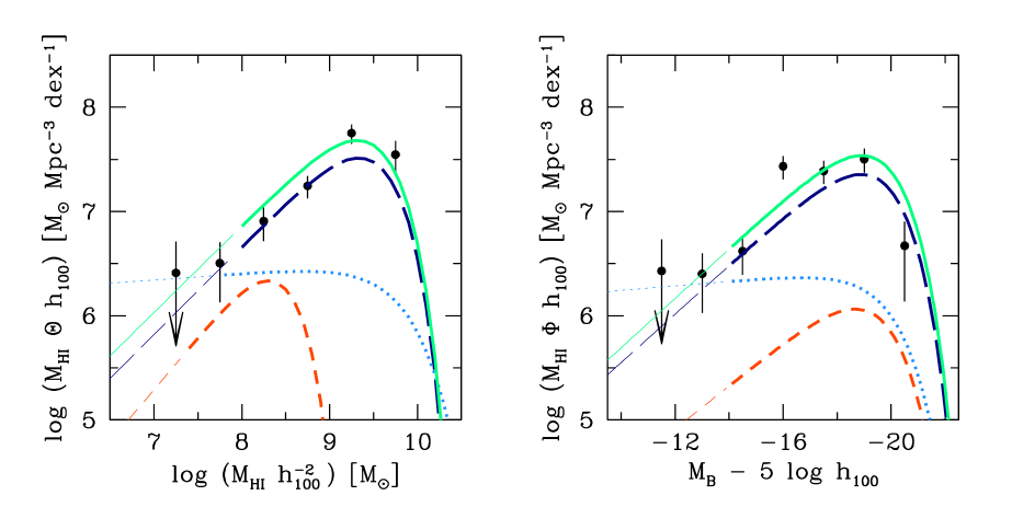
Figure 3: Left panel: Space density of H i mass per decade contained in objects of different mass. Right panel: Space density of H i mass per mag contained in objects of different absolute magnitude. Lines are as in Fig. 1. Most of the H i at the present epoch is locked up in luminous galaxies with high H i masses. Dwarfs seem to contribute very little to the gas density.

Figure 3 shows how this gas density is distributed over different H i masses and different luminosities. As in Fig. 1 the lines represent converted LFs [23] for different morphological types. It is clear that the gas density in the local Universe is dominated by massive galaxies in the range $10^{9}~{}\mbox{${\rm M}_{\odot}$}<\mbox{$M_{\rm HI}$}<10^{10}~{}\mbox{${\rm M}_{\odot}$}$, with high luminosities. The presently known dwarf galaxies are minor contributors to $\Omega_{\rm g}$ since galaxies with H i masses below $10^{8}~{}\mbox{${\rm M}_{\odot}$}$ are responsible for only $\sim 20\%$ of the gas density.

Although the run of $\Omega_{\rm g}$ with redshift is generally considered to reach a peak at $z\approx 3$ and then declines until $z=0$, the most recent (preliminary) results from Turnshek et al. [40] show that $\mbox{$\Omega_{\rm g}$}(z)$ is consistent with no evolution from $z=3$ to $z\approx 0.15$. Still, the $z=0$ point, evaluated via the 21cm in emission, lies approximately a factor of six lower. If, like the AHiSS results suggest, most of the neutral gas indeed resides in large spirals, the identification of galaxies responsible for damped Ly$\alpha$ absorption would be trivial. Rao et al. [28] show that the opposite is true: none of the galaxies in the vicinity of the quasar in which two nearby absorbers are found are luminous spirals. Also at higher redshifts there are indications that dwarf galaxies contribute significantly to the cross section of damped Ly$\alpha$ absorbers. Le Brun et al. [19] find that most of the optical counterparts of damped Ly$\alpha$ systems at high redshift are dwarf galaxies. Matteucci et al. [22] conclude on the basis of chemical evolution models that most damped Ly$\alpha$ absorbers are in fact dwarf galaxies.

There are two possible solutions to this $z=0$ conundrum. Either there has been strong evolution at very low redshift, implying that most of the star formation has occurred over the last few Gyrs, or estimates of the gas density at $z=0$ from the 21cm line are still incomplete. At least in the range $\mbox{$M_{\rm HI}$}>10^{8}~{}\mbox{${\rm M}_{\odot}$}$ most authors agree well on the shape and normalization of the HiMF and derivations based on optically selected and H i selected galaxies are consistent. If an incompleteness of the HiMF exists it must be in the tail of the HiMF. The question to answer is therefore: are there large populations of gas rich dwarf galaxies or H i clouds with typical 21cm fluxes undetectable in present surveys?

In this light it is interesting to note that are recent claims of a sharply rising LF, typically faintward of $M=-16$ (see [21]). The galaxies responsible for this upturn are generally of late morphological type, with blue colors and low optical surface brightness. These are the galaxies normally regarded as being rich in neutral gas (see also [31]).

Another interesting recent result comes from Blitz et al. [3], who argue that many of the high velocity clouds (HVCs) populated around the Milky Way Galaxy are actually H i clouds with masses of a few times $10^{7}~{}\mbox{${\rm M}_{\odot}$}$ distributed trough the Local Group. Their integrated mass may account to as much as $10^{11}~{}\mbox{${\rm M}_{\odot}$}$.

4 The Faint Tail

Obviously, determining the faint tail of the HiMF deserves special attention. An accurate determination below $\mbox{$M_{\rm HI}$}=10^{7}~{}\mbox{${\rm M}_{\odot}$}$ has proven to be an extremely difficult exercise in blind surveys. For the Parkes Multibeam survey, the largest H i survey to date, the limiting depth for a galaxy with $10^{6}~{}\mbox{${\rm M}_{\odot}$}$ of H i is 1 Mpc [38]. This estimate assumes that the profile width of the galaxy is 200 $\rm km\,s^{-1}$, while in reality the profile width for these tiny H i masses will probably be much smaller, implying that the same flux is spread over fewer channels which makes the galaxy more easily detectable. Even if the limiting depth is 2 Mpc, the maximum search volume for $10^{6}~{}\mbox{${\rm M}_{\odot}$}$ H i masses is ${\cal V}=\frac{1}{3}\Omega\,D^{3}\approx 17\,\rm Mpc^{3}$, where $\Omega$ is the solid angle. The search volume will therefore be confined to the Local Group environment.

For a blind H i survey, the survey volume as a function of H i mass can be evaluated in the following way. The minimal detectable H i mass $\mbox{$M_{\rm HI}$}_{\rm,min}$ for a $5\sigma$ detection can be expressed as $236\times 5\sigma\Delta VD^{2}$, where $\sigma$ is the noise in the detection spectra in mJy, $\Delta V$ is the profile width in km/s and $D$ is the distance to the source in Mpc. Assuming optimal smoothing of the survey spectra, the noise goes as $\sigma\propto\Delta V^{-1/2}$, and therefore $\mbox{$M_{\rm HI}$}_{\rm,min}\propto D^{2}\Delta V^{1/2}$. The limiting depth, the maximum distance at which a source could be placed and still be detected, is then given by $D_{\rm c}\propto\mbox{$M_{\rm HI}$}^{1/2}\Delta V^{-1/4}$. The H i mass is related to the profile width via the Tully-Fisher relation and the relation between H i mass and optical luminosity. The “H i Tully-Fisher relation” goes as $\Delta V\propto\mbox{$M_{\rm HI}$}^{1/3}$ [4]. The limiting depth is therefore $D_{\rm c}\propto\mbox{$M_{\rm HI}$}^{5/12}$. Finally, since the total search volume is ${\cal V}=\frac{1}{3}\Omega\,D_{\rm c}^{3}$, we derive ${\cal V}\propto\mbox{$M_{\rm HI}$}^{5/4}$. In contrast to optical surveys, H i surveys are conducted with a limited bandwidth which imposes a hard upper limit to the limiting depth for massive galaxies. The surveys volume therefore reaches a maximum for H i masses that can be detected at the redshift corresponding to the receiver’s frequency limit and does not increase for higher masses. The sensitivity curve, the inverse of the survey volume, is therefore a straight line with slope $-1.25$, leveling off to a straight line for H i masses which can be seen all trough the survey volume. The decreasing part is parallel to an HiMF with a slope of $-2.25$.

The number of detections in a survey can be estimated by taking the integral over the HiMF times the survey volume:

$${\cal N}=\int_{0}^{\infty}\,\Theta(\mbox{$M_{\rm HI}$}){\cal V}(\mbox{$M_{\rm HI}$})\,d\mbox{$M_{\rm HI}$}.$$

Graphically, this number can be regarded as the surface enclosed by the HiMF and the sensitivity curve (see Fig. 2). If $\alpha<-2.25$ the surface would not be closed and the number of detections would be infinite. For the HiPASS survey, the instrumental depth limit set by the bandwidth of the receiving system is $127~{}h^{-1}_{100}~{}\rm Mpc$ and the covered solid angle is $\Omega=6.5$. If then the Schechter parameters for the HiMF found by Zwaan et al. [43] are used, the number of detections for this survey will be ${\cal N}=2516$ galaxies, increasing the size of existing samples by a factor of 30. The statistics will be dominated by $M^{*}_{\rm HI}$ galaxies: more than 70% of the detected galaxies will have H i masses in the range $10^{9}~{}\mbox{${\rm M}_{\odot}$}<\mbox{$M_{\rm HI}$}<10^{10}~{}\mbox{${\rm M}_{\odot}$}$. If the faint slope of $\alpha=-1.2$ extends to the lowest masses, only $4\pm 2$ galaxies with H i masses below $10^{7}~{}\mbox{${\rm M}_{\odot}$}$ will be detected. This number rises to 13 if the latest value of $\alpha=-1.35$ quoted by Kilborn [17] is used. If the slope is much steeper than currently assumed, for example $\alpha=-1.7$ below $\mbox{$M_{\rm HI}$}=10^{8}~{}\mbox{${\rm M}_{\odot}$}$, in concordance with the estimates of the optical LF, the number of dwarfs will be 57, high enough to reliably determine the shape of the HiMF down to $\mbox{$M_{\rm HI}$}=10^{6}~{}\mbox{${\rm M}_{\odot}$}$.

Thanks to their smaller dishes, synthesis instruments like the WSRT and the VLA sample larger volumes per single pointing than the Parkes telescope. These instruments may be more useful for constraining the faint end. If the accessible bandwidth is 20 MHz the sampled volume will be ${\cal V}=\frac{1}{3}D_{\rm max}^{3}({\rm FWHM}/2)^{2}\pi=1.5~{}\rm Mpc^{3}$ per single pointing. In 24 hours H i masses of $10^{7}~{}\mbox{${\rm M}_{\odot}$}$ will be detectable throughout the volume. Adopting the HiMF parameters for field galaxies from the AHiSS we estimate that the number of detections will be approximately half a galaxy per pointing of 24 hours. The statistics will be dominated by galaxies in the range $10^{7}~{}\mbox{${\rm M}_{\odot}$}<\mbox{$M_{\rm HI}$}<10^{8}~{}\mbox{${\rm M}_{\odot}$}$, two orders of magnitude lower in H i mass than in the HiPASS survey. If again the HiMF with $\alpha=-1.7$ for $\mbox{$M_{\rm HI}$}<10^{8}~{}\mbox{${\rm M}_{\odot}$}$ is assumed, the number of detections in the $6$ to $6.5~{}\mbox{${\rm M}_{\odot}$}$ bin will be 0.05. In order to get a statistically significant result many months of observing time will be required. Apparently, determining the faint end slope of the HiMF below $10^{7}~{}\mbox{${\rm M}_{\odot}$}$ in the field is not possible with the current generation of radio telescopes.

A way to overcome the poor statistics and the uncertain volume corrections is to study nearby groups of galaxies. Typical overdensities of these groups are a factor 25 of the cosmic mean, which improves the statistics significantly. Furthermore, the distances of groups can be determined quite accurately using Cepheid measurements or by photometry on the brightest resolved stars of only one or a few group members, or by using the potent method [2]. Studies of the HI content of galaxies in different environments have shown that the shape of the HiMF for $\mbox{$M_{\rm HI}$}>10^{8}$ is independent of cosmic density. This finding justifies the study of the HiMF in groups of galaxies, although it is possible that the faint tail may depend on environment.

Acknowledgements.  Thanks to F. Briggs, R. Swaters and E. de Blok for comments on the text. Financial support was received from the EC (TMR) and the LKBF.

References

- [1] Barnes, D. G., Staveley-Smith, L., Webster, R. L., & Walsh, W. 1997, MNRAS 288, 307
- [2] Bertschinger, E., Dekel, A., Faber, S. M., Dressler, A., & Burstein, D. 1990, Astrophys. J. 364, 370
- [3] Blitz, L., Spergel, D. N., Teuben, P. J., Hartmann, D., & Burton, W. B. 1998, astro-ph/9803251
- [4] Briggs, F. H., & Rao, S. 1993, Astrophys. J. 417, 494
- [5] Dalcanton, J. J., Spergel, D. N., Gunn, J. E., Schmidt, M., & Schneider, D. 1997, Astrophys. J. 114, 635
- [6] de Blok, W. J. G. 1997, Ph.D. Thesis, University of Groningen
- [7] Dickey, J. M. 1997, Astron. J. 113, 1939
- [8] Disney, M. J. 1976, Nature 263, 573
- [9] Efstathiou, G., Ellis, R. S., & Peterson, B. A. 1988, MNRAS 231, 479
- [10] Fisher, J. R., & Tully, R. B. 1975, Astr. Astrophys. 44, 151
- [11] Fisher, J. R., & Tully, R. B. 1981, Astrophys. J. 243, L23
- [12] Haynes, M. P., & Roberts, M. S. 1979, Astrophys. J. 227, 767
- [13] Henning, P. A. 1992, Astrophys. J. Suppl. Ser. 78, 365
- [14] Henning, P. A. 1995, Astrophys. J. 450, 578
- [15] Henning, P. A., Kraan-Korteweg, R. C., Rivers, A. J., Loan, A. J., Lahav, O., & Burton, W. B. 1998, Astron. J. 115, 584
- [16] Hoffman, G. L., Lewis, B. M., Helou, G., Salpeter, E. E., & Williams, B. M. 1989, Astrophys. J. Suppl. Ser. 69, 65
- [17] Kilborn, V. A. 1998, these proceedings
- [18] Krumm, N., & Brosch, N. 1984, Astron. J. 89, 1461
- [19] Le Brun, V., Bergeron, J., Boissé, P., & Deharveng, J. 1997, Astr. Astrophys. 321, 733
- [20] Lo, K. Y., & Sargent, W. L. W. 1979, Astrophys. J. 227, 756
- [21] Loveday, J. 1998, these proceedings
- [22] Matteucci, F. 1998, these proceedings
- [23] Marzke, R. O., da Costa, L. N., Pellegrini, P. S. C., Willmer, C. N. A., & Geller, M. J. 1998, astro-ph/9805218
- [24] McGaugh, S. S. 1996, MNRAS 280, 337
- [25] McMahon, P. M. 1993, Ph.D Thesis, Columbia University
- [26] Natarajan, P., & Pettini, M. 1997, MNRAS 291, 28
- [27] Rao, S., & Briggs, F. H. 1993, Astrophys. J. 419, 515
- [28] Rao, S., & Turnshek, D. A. 1998, astro-ph/9805093
- [29] Sandage, A., Tammann, G. A., & Yahil, A. 1979, Astrophys. J. 232, 352
- [30] Schmidt, M. 1968, Astrophys. J. 151, 393
- [31] Schneider, S. E. 1998, these proceedings
- [32] Schombert, J. M., Bothun, G. D., Schneider, S. E., & McGaugh, S. S. 1992, Astron. J. 103, 1107
- [33] Shostak, G. S. 1977, Astr. Astrophys. 54, 919
- [34] Somerville, R. S., & Primack, J. R. 1998, astro-ph/9802268
- [35] Sorar, E. 1994, Ph.D. Thesis, University of Pittsburgh
- [36] Spitzak, J. G. 1996, Ph.D. Thesis, University of Massachusetts
- [37] Sprayberry, D., Impey, C. D., Irwin, M. J., & Bothun, G. D. 1997, Astrophys. J. 482, 104
- [38] Staveley-Smith, L., Wilson, W. E., Bird, T. S., Disney, M. J., Ekers, R. D., Freeman, K. C., Haynes, R. F., Sinclair, M. W., Vaile, R. A., Webster, R. L., & Wright, A. E. 1996, PASA, 13, 243
- [39] Szomoru, A., Guhathakurta, P., van Gorkom, J. H., Knapen, J. H., Weinberg, D. H., & Fruchter, A. S. 1994, Astron. J. 108, 491
- [40] Turnshek, D. A. 1997, in Structure and Evolution of the Intergalactic Medium from QSO Absorption Line Systems, ed. Petitjean & Charlot
- [41] van Zee, L., Haynes, M. P., & Giovanelli, R. 1998, Astron. J. 109, 990
- [42] Willmer, C. N. A. 1997, Astron. J. 114, 898
- [43] Zwaan, M. A., Briggs, F. H., Sprayberry, D., & Sorar, E. 1997, Astrophys. J. 490, 173
- [44] Zwaan, M. A., Sprayberry, D., & Briggs, F. H. 1998, in preparation