THE SOLAR INTERNAL ROTATION FROM GOLF SPLITTINGS

Abstract

The low degree splittings obtained from one year of GOLF data analysis are combined with the MDI medium-l 144-day splittings in order to infer the solar internal rotation as a function of the radius down to $0.2R_{\odot}$. Several inverse methods are applied to the same data and the uncertainties on the solution as well as the resolution reachable are discussed. The results are compared with the one obtained from the low degree splittings estimated from GONG network.

Key words: solar core rotation; inversion.

1. INTRODUCTION

The rotation of the solar core is an important open question that can be addressed by using spatial data from SOHO. In particular, GOLF experiment is dedicated to the observation of low-degree oscillations which sound the core. Here we use the GOLF frequency splittings (??) obtained from one year of observation beginning on April 11th 1996 together with the MDI 144-day splittings for degree up to $l=250$ (??). For comparison we have also used the GONG splittings of low-degree modes obtained (??) from 1 year of ground-based observations (August 1995- August 1996).

Figure 1.: Sideral sectoral splittings (GOLF) and $a_{1}$ coefficients (MDI and GONG) with their formal errors as a function of the turning points of the modes.

Figure 1 shows the GOLF sectoral splittings with their formal errors whereas for MDI and GONG data the figure shows the $a_{1}$ coefficients of the expansion of the splittings on ?? polynomials. These two quantities (sectoral splittings and $a_{1}$ coefficients) may differ slightly in theory for $l>1$ because of the latitudinal dependence of the solar rotation. In Section 2. we briefly recall how the 2D inverse problem related to the internal rotation can be reduced to a 1D problem for either the $a_{1}$ coefficients or the sectoral splittings and how in both cases the use of sectoral splittings may need some a-priori assumptions on the rotation. Then, Section 3. presents the different inverse methods used and, finally, we discuss the results obtained in Section 5.

2. FROM THE 2D TO THE 1D INVERSE PROBLEM

For low rotation the frequency of a mode of radial order $n$ and degree $l$ is splitted in $2l+1$ components of azimuthal order $m=-l,..+l$ and the splittings $\Delta\nu_{nlm}\equiv{\nu_{nlm}-\nu_{nl0}\over m}$ are given by:

$$\Delta\nu_{nlm}\!=\int_{0}^{1}\!\!\int_{0}^{R_{\odot}}\!K_{nlm}(r,\mu)\Omega(r,\mu)drd\mu,$$ (1)

where $\Omega(r,\mu)$ is the unknown rotation rate versus depth $r$ and colatitude $\theta$ ($\mu=\cos\theta$) and $K_{nlm}(r,\mu)$ the so-called rotational kernels calculated for each mode from oscillation eigenfunctions of an equilibrium solar model.

In order to investigate the rotation below $0.4R_{\odot}$ where the latitudinal dependence is particularly not well constrained because of the few azimuthal orders provided by the low $l$ degree modes, one may want to simplify the problem and reduce it to 1D problem in radius. As a matter of fact 2D inversions are usually not able to peak averaging kernels in both radial and latitudinal direction below $0.4R_{\odot}$ and two different 1D approximations of Equation 1 are used instead.

2.1. 1D relation for sectoral splittings

One possibility in order to obtain a 1D integral relation is to search for the rotation rate at a given latitude only. Since the most constrained zone is the equatorial one, we try to investigate only the equatorial rotation rate. For this purpose we use the approximation

$$K_{nlm}(r,\mu)\simeq K_{nl}(r)P_{l}^{m}(\mu)^{2}$$ (2)

where $K_{nl}(r)$ are radial kernels (e.g. ??) and $P_{l}^{m}(\mu)$ are Legendre functions normalized such that $\int_{-1}^{1}P_{l}^{m}(\mu)^{2}d\mu=1$, and which satisfy the following property for $m=l$:

$$P_{l}^{l}(\mu)^{2}=C_{l}(1-\mu^{2})^{l}\ \ \ C_{l}={(2l+1)!\over 2^{2l+1}(l!)^{2}}$$ (3)

This shows that, for high-degrees $l$, the major contribution to sectoral splittings $\Delta\nu_{nll}$ comes from the equatorial rotation rate $\tilde{\Omega}_{eq}(r)=\Omega(r,\mu=1)$. This leads to the 1D integral approximation:

$$\Delta\nu_{nll}\simeq\int_{0}^{R_{\odot}}K_{nl}(r)\tilde{\Omega}_{eq}(r)dr$$ (4)

Nevertheless this approximation is valid only for high degrees $l$. For lower degrees the sectoral splittings are sensitive not only to the equatorial rotation but also to the rotation rate in a large angular domain around the equator. The extent of this domain and the influence of this approximation on the estimation are discussed in ??.

2.2. 1D relation for $a_{1}$ coefficients

Some experiments like GONG and MDI produce a small number of the so-called a-coefficients of splittings expansions on a set of orthogonal polynomials (??). Assuming that the relation between individual splittings and these coefficients is linear, an equation similar to Equation 1 can be established by computing the appropriate kernels $K_{nlj}^{a}(r,\mu)$ related to each $a^{nl}_{j}$-coefficients for odd indices $j$ (see e.g. ??). Furthermore it has been shown by ?? that the expansion of the splittings in orthogonal polynomials corresponds to an expansion of $\Omega(r,\mu)$ such that:

$$\Omega(r,\mu)=\tilde{\Omega}_{1}(r)+\sum_{j=3,5...}\tilde{\Omega}_{j}(r){dP_{j}(\mu)\over d\mu},$$ (5)

where $P_{j}$ are the Legendre polynomials. This forms the so called 1.5D problem where each $a_{j}$-coefficient is related to the expansion function of the same index through a 1D integral. Therefore the first term of the expansion Equation 5 which do not depend on the latitude can be related to the $a_{1}$-coefficients through:

$$a^{nl}_{1}=\int_{0}^{R_{\odot}}K_{nl}(r)\tilde{\Omega}_{1}(r)dr$$ (6)

The radial kernel $K_{nl}(r)$ is the same as in Equation 2 but, from Equation 5, the function $\tilde{\Omega}_{1}(r)$ obtained by inverting $a_{1}$ coefficients corresponds to the searched rotation rate only where the rotation do not depend on the latitude. Otherwise it corresponds to some average over latitudes that can be estimated by looking at the corresponding 2D averaging kernel (cf. Section 4. and Figure 3).

3. INVERSE METHODS

We have used two kinds of inverse methods for solving the 1D integral equations.

1. A Regularized Least-Squares (RLS) method with Tikhonov regularization (see e.g. ??). This is a global method which gives a solution at all depths which fits the data at the best in the least square sense. This is a linear method and then the value of the rotation obtained at any radius $r_{0}$ is a linear combination of the data:

   $$\hat{\Omega}_{\left|{eq\atop 1}\right.}\!(r_{0})=\sum_{nl}C_{nl}(r_{0})\left|{\Delta\nu_{nll}\atop a_{1}^{nl}}\right.$$ (7)

   By replacing in Equation 4 or 6 we obtain:

   $$\hat{\Omega}_{\left|{eq\atop 1}\right.}\!(r_{0})=\int_{0}^{R_{\odot}}\left(\sum_{nl}C_{nl}(r_{0})K_{nl}(r)\right)\tilde{\Omega}_{\left|{eq\atop 1}\right.}\!(r)dr$$ (8)

   The function in parenthesis is called 1D averaging kernel at $r_{0}$, $\kappa(r,r_{0})$. The result obtained at $r_{0}$ will be easier to interpret as a local average of the rotation when this kernel is well-peaked and without strong oscillatory behaviour.

2. Two ‘local’ methods which search directly the coefficients $C_{nl}(r_{0})$ which are able to peak the averaging kernel near $r_{0}$. The two methods differ essentially in the way to localize the averaging kernel. The SOLA (Subtractive Optimally Localized Average) method (??) fits the averaging kernel to a Gaussian function of given width whereas the MOLA method (Multiplicative OLA) (??) simply gives high weights in the minimization process to the part of the averaging kernel which are far from the target radius. In both case we use a regularizing parameter in order to establish a balance between the resolution and the error magnification reached at the target $r_{0}$.

4. HOW TO USE $l=2,3$ SECTORAL SPLITTINGS?

As already quoted, GOLF data for $l=2,3$ are not $a_{1}$ coefficients but sectoral splittings. Therefore one may want to use the Equation 4 in order to infer the equatorial rotation rate. There are two difficulties with this approach:

Figure 2.: Difference in sectoral splittings computed from Equation 1 and from the 1D approximation Equation 6 for a given 2D rotation profile resulting from a 2D RLS inversion of MDI data. The difference is around $12$nHz for $l=1$, $8$nHz for $l=2$, $6$nHz for $l=3$. This is due to the fact that for low $l$, $P_{l}^{l}(\mu)$ extend far from the equator and therefore low-degree sectoral modes are more sensitive to the latitudinal dependency of the rotation in the convection zone than other sectoral modes.

1. As already mentioned in Section 2.1., the relation Equation 4 is not valid for low-degree $l$ and therefore may not be suited for the determination of the core rotation. This may be corrected by assuming that the latitudinal dependence of the rotation rate (i.e. $\tilde{\Omega}_{j}(r)$ $j=3,5..$) is known (taken from some previous 2D inversions for example). With this assumption, we can correct the observed sectoral splitting prior to inversion by adding for each mode the difference between the sectoral splittings computed from Equation 1 and from Equation 4. This difference is plotted on Figure 2 as a function of the degree $l$.

2. MDI data do not provide the sectoral splittings for high $l$ but only upon $18$ odd indexed $a$-coefficients. This number of coefficients is however high enough so that taking their sum as sectoral splittings is a good approximation. Nevertheless, the error on these sums (called ‘truncated sectoral splittings’ in the following) is always higher than the error on $a_{1}$ alone.

Another possibility is to consider the sectoral splittings $l=2,3$ as $a_{1}$ coefficients at first approximation. In this approach we do not need to correct the data because Equation 6 is valid even for low degrees. Nevertheless, we can also use other dataset (MDI for example) or our knowledge of the latitudinal dependence of the rotation (taken from a previous 2D inversion for example) in order to estimate $a_{3}$ for modes $l=2$ and $a_{3}$, $a_{5}$ for modes $l=3$.

With the same approximation as in Equation 2 we can write for the a-coefficients:

$$K^{a}_{nlj}(r,\mu)\simeq K_{nl}(r)Q_{lj}(\mu)$$ (9)

so that, for both approaches, the solution obtained at $r_{0}$ can ever be seen as an average of the rotation of the form:

$$\hat{\Omega}(r_{0})\!\!=\!\!\int\!\!\int\!\!\Bigl{(}\sum_{nl}C_{nl}(r_{0})K_{nl}(r)W_{l}(\mu)\Bigr{)}\Omega(r,\mu)drd\mu$$ (10)

The 2D averaging kernels (defined by the term in parentheses in Equation 10) can therefore be estimated from the 1D averaging kernels Equation 8 obtained at a target location $r_{0}$ by adding the angular part $W_{l}(\mu)$ of the 2D rotational kernel that corresponds to the data really inverted.

Figure 3 shows on the left the 2D averaging kernels (defined by the term in parentheses in Equation 10) obtained at $r_{0}=0.2R_{\odot}$ by inverting GOLF sectoral splittings together with MDI ‘truncated sectoral’ splittings i.e.:

$$W_{l}(\mu)=\left\{\begin{array}[]{ll}P_{l}^{l}(\mu)^{2}&\mbox{for }l\leq 3\\ &\\ \displaystyle\sum_{j=1}^{jmax}Q_{lj}(\mu)&\mbox{for }l>3\end{array}\right.$$ (11)

whereas, on the right, it shows the 2D averaging kernel obtained at the same target location by inverting MDI $a_{1}$ coefficients together with GOLF sectoral splittings for $l=1,2,3$ i.e.:

$$W_{l}(\mu)=\left\{\begin{array}[]{ll}P_{l}^{l}(\mu)^{2}&\mbox{for }l\leq 3\\ &\\ Q_{l1}(\mu)={3\over 2}(1-\mu^{2})&\mbox{for }l>3\end{array}\right.$$ (12)

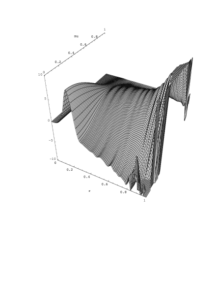
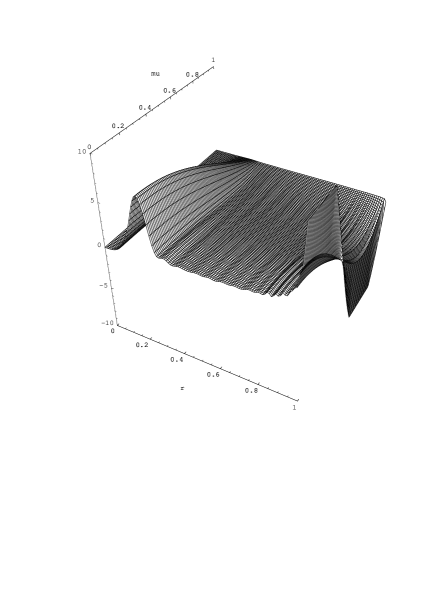
Figure 3.: 2D averaging kernels for 1D inversions computed at $r_{0}=0.2R_{\odot}$ (see Section 4). Left panel: inversion of GOLF sectoral splittings for $l\leq 3$ with MDI ‘truncated sectoral’(see text) splittings for $l>3$. Right panel: inversion of GOLF sectoral splittings for $l\leq 3$ with MDI $a_{1}$ coefficients. The peaks near the surface are truncated on the plot for clarity.

The two corresponding 1D averaging kernels (cf. Figures. 6 and 5) are the integral over latitude of these 2D kernels and are very similar: well localized near $0.2R_{\odot}$ and without contributions near the surface. The angular part of the averaging kernel for sectoral splittings strongly depend on the degree $l$ and this leads to the oscillatory behaviour of the 2D kernel with very high peaks near the surface. From this plot it is clear that the interpretation of the result obtained by inverting sectoral splittings is possible only if we have already a good knowledge of the latitudinal dependence of the rotation. Furthermore, as already pointed out, this knowledge is needed in order to correct the low-degree sectoral splittings for which the 1D approximation is not valid. At the opposite, for $a_{1}$ coefficients $Q_{l1}(\mu)$ is independent of $l$ (cf. Equation 12). Therefore the surface oscillatory behaviour on the right panel of Figure 3 comes only from the use of sectoral splittings for $l=2,3$. In this case, the knowledge of the rotation profile is needed only near the surface in order to interpret the result.

We can summarize the results of this study in few points:

1. It is clear that it is better to use $a_{1}$ coefficients than sectoral splittings when we have them.

2. In the case of GOLF data, we have access only to sectoral splittings for $l=2,3$. If we want to use them, it seems more reasonable to try to correct them by doing some assumptions on $a_{3}$ and $a_{5}$ for these modes and to use the exact 1D integral rather than correcting all the modes in order to use the approximated 1D integral Equation 4.

3. In both approaches we can in principle obtain a result easy to interpret if the latitudinal variation of the rotation is assumed to be known exactly. But by inverting $a_{1}$ for $l>3$ together with sectoral splittings for $l<3$, we just have to make assumptions on the surface rotation.

4. Several ways can be followed for correcting the results obtained by using sectoral splittings in $a_{1}$ inversions. We can either

   • take a guess rotation and integrating its surface part with the 2D kernel in order to correct the solution after the inversion or

   • take $a_{3}$ and $a_{5}$ from other datasets or

   • calculate these coefficients from the guess rotation and subtract them from sectoral splittings before the inversion.

   The best is probably to compare the effects of all these corrections and to compare with the inversion of the corrected ‘truncated sectoral’ splittings. In any case assumptions are needed on the latitudinal dependence of the rotation. As this dependence can not be known exactly it should be interesting to study in future works how these assumptions increase the uncertainties on the solution.

The next Section shows some preliminary results obtained with these different approaches for the use of the combined MDI and GOLF data.

5. RESULTS AND DISCUSSIONS

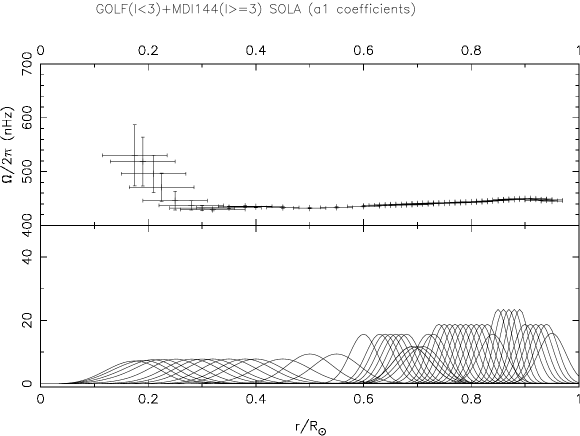
Figure 4.: SOLA inversion of MDI $a_{1}$ coefficients and GOLF $l=1,2$ sectoral splittings. The corresponding 1D averaging kernels are shown below each point of the solution. Vertical and horizontal error bars represent respectively the error and the resolution defined as the FWHM of the averaging kernel.

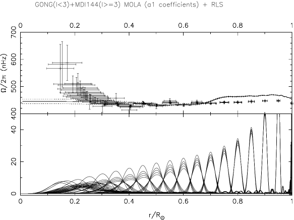
Figure 5.: MOLA inversion of the same data as in Figure 4. Five regularizing parameters have been used at each target location. The full line shows an RLS inversion of the corrected ‘truncated sectoral splittings’ (see text) and the dotted line gives 1$sigma$ errors on this solution.

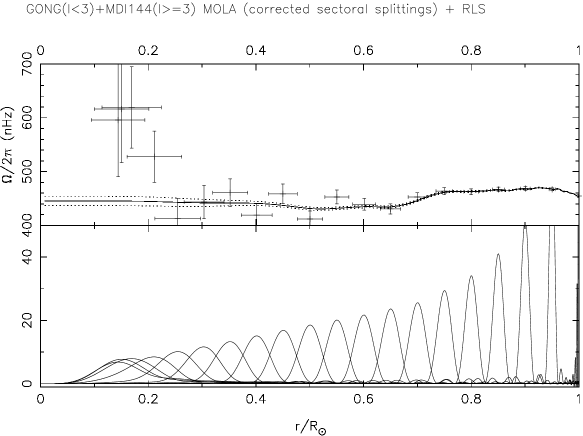
Figure 6.: MOLA and RLS inversion of the corrected ‘truncated sectoral splittings’. Low regularization has been used in MOLA inversion.

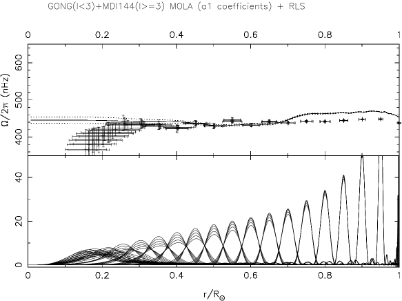
Figure 7.: The same as Figure 5 but using GONG $a_{1}$ coefficients for l=1,2,3 instead of GOLF sectoral splittings.

In this preliminary work, we have chosen, as a first step, to use only $l=1,2$ GOLF sectoral splittings in order to reduce the difficulties discussed in the previous sections. Figures 4 and 5 show the results obtained by inverting the $a_{1}$ coefficients together with $l=2$ sectoral splittings by using SOLA and MOLA inverse methods. In SOLA method the trade-off parameter is rescaled at each target location to obtain more localized averaging kernels. For MOLA method five trade-off parameters have been used at each target location. In the case of low regularization MOLA averaging kernels have some small oscillatory parts. The two methods fall in good agreement down to $0.20R_{\odot}$ where the rotation rate increases up to $500\pm 60$nHz. Below $0.15R_{\odot}$ both methods fail to peak kernels. On Figure 5 we have shown a RLS solution obtained by inverting sectoral splittings. As expected the two solutions ($\hat{\Omega}_{eq}$ and $\hat{\Omega}_{1}$) differ in the convection zone where the rotation rate vary with latitude. In the core, it is difficult to use RLS method because it is a global method and if one try to obtain a well localized averaging kernel down to $0.2R_{\odot}$ then we have to decrease the regularization and the solution becomes very oscillating everywhere with big error bars. With an optimal L-curve choice of the regularizing parameter the solution is constant ($445nHz$ see Figure 5) below $0.4R_{\odot}$ but averaging kernels (not shown on the plot) computed below this point are still localized near $0.4R_{\odot}$ so that, with this method, there is no conclusion on the core rotation in terms of weighted average of the true rotation. Nevertheless, we can use this solution and look at the residuals for each mode. The global normalized $\chi^{2}$ of the inversion is 1.2. Now, if we look only at low-degree GOLF modes, the ‘partial normalized $\chi^{2}$’ is around 0.5 showing that within error bars GOLF data are in good agreement with a constant rotation below $0.4R_{\odot}$ and that GOLF errors are probably not underestimated. Furthermore, looking at the residuals for each individual splittings can help in the signal analysis by pointing out some modes with high residuals that may be reanalyzed in order to become more confident on the result.

Following the discussion of the previous sections we have also inverted the sectoral (or ‘truncated sectoral’) splittings corrected by using the latitudinal dependence of the rotation found by a 2D RLS inversion of MDI data. The result is shown on Figure 6 in the case of low regularization. As expected the solution corresponds to the equatorial rotation profile as found by the RLS method in the convection zone and the error bars increase compared to the use of $a_{1}$ coefficients alone. The solution in the core is a little bit higher than found by $a_{1}$ inversion but remains compatible within error bars showing also an increasing rotation rate below $0.025R_{\odot}$.

We have also tried to include GOLF $l=3$ sectoral splittings in our inversions. This leads to a more important increase of the rotation rate below $0.2R_{\odot}$ (around $700\pm 100$ nHz). But in this case more work is needed in order to become more confident in our result. In particular, in that case, we have to test the effects of the various corrections suggested in Section 4. and to look at their influence on the estimation of the uncertainties on the core rotation.

Finally, we have done the same analysis with GONG low-degree data (??). In the case of GONG data we have $a_{1}$ coefficients so that, as quoted before, it may be more suited to carry an inversion of these coefficients using Equation 6 rather than using the ‘truncated sectoral’ splittings. In order to compare the result with the previous ones, the GONG $a_{1}$ coefficients for low-degrees have been used together with the MDI $a_{1}$ coefficients of higher degree modes. Figure 7 shows that these data tend to produce a slightly decreasing rotation rate below $0.3R_{\odot}$. Therefore there is still a relatively important difference between the solutions obtained with the different low-degrees data. These differences are significant only if the error bars obtained on the solutions are not underestimated and may be related to the important dispersion of individual splittings measurements (cf. Figure 1). Furthermore, we must notice that whereas MDI and GOLF splittings are for the same year of observations(5/96-5/97), the GONG data are for the year before (5/95-5/96) and therefore the results may not be directly compared. Therefore this result needs to be confirmed in future works and we have also to inverse GONG $a_{1}$ coefficients for all the modes which should be a more self-consistent dataset.

6. FUTURE WORKS AND SOME QUESTIONS

The problem of inferring the core physics remains one of the most important still open question that can be addressed by helioseismology. It is therefore very important, as a first step, to be sure that different ‘inverters’ using different inverse methods can reach similar conclusions when they use the same datasets. This was the goal of this work in collaboration between ‘inverters’ within the GOLF team and we have shown that the different approaches of the inversion are coherent. After this preliminary work several questions need to be addressed, for example:

• Can we obtain reliable results below $0.2R_{\odot}$ with actual datasets?

• How the results in the core are sensitive to the data used for medium $l$ splittings?

• Can we explain the differences between the results obtained with different data by a systematic bias in some splitting measurements or by underestimated errors in a few number of individual splittings?

• Can these results (obtained with inverse methods) be confirmed by using forward methods often used for the core rotation problem (??; ??)?

References

- Backus & Gilbert 1970 Backus, G.E., Gilbert, J.F. 1970, Phil. Trans. R. Soc. Lond. A.266, 123
- Charbonneau et al. 1998 Charbonneau, P., Tomczyk, S., Schou, J., Thompson, M.J. 1998, ApJ, 496, 1015
- Corbard 1997 Corbard, T. 1997, proceedings of 9th IRIS meeting (Capodimonte, Italy, July 1997)
- Cuypers 1980 Cuypers, J. 1980, A&A, 89, 207
- Gizon 1998 Gizon, L., 1998, In: Provost, J., Schmider, F.X. (eds.) IAU Symp. 181: Sounding Solar and Stellar Interior (poster volume). OCA & UNSA, Nice, p. 89
- poster 1.39, these proceedings 1998 GOLF team, poster 1.39, 1998, these proceedings
- Pijpers & Thompson 1992 Pijpers, F.P., Thompson, M.J. 1992, A&A, 262, L33
- Pijpers 1997 Pijpers, F.P. 1997, A&A, 326, 1235
- Rabello-Soares & Appourchaux 1998 Rabello-Soares, C., Appourchaux, T. 1998, these proceedings
- Ritzwoller & Lavely 1991 Ritzwoller, M.H., Lavely, E.M. 1991, ApJ, 403, 810
- Schou et al. 1998 Schou, J., et al. 1998, ApJ, submitted