The stellar dynamics and mass of NGC 1316  using the radial velocities of Planetary Nebulae

Abstract

We present a study of the kinematics of the outer regions of the early-type galaxy NGC 1316, based on radial velocity measurements of 43 planetary nebulae as well as deep integrated-light absorption line spectra.

The smoothed velocity field of NGC 1316 indicates fast rotation at a distance of 16 kpc, possibly associated with an elongated feature orthogonal to the inner dust lanes. The mean square stellar velocity is approximately independent of radius, and the estimated total mass of the system is $2.9\times 10^{11}M_{\odot}$ within a radius of 16 kpc, implying an integrated mass–to–light ratio of M/L${}_{B}\simeq 8$.

1 Introduction

The use of planetary nebulae (PNe) to measure radial velocities in the outer regions of early-type galaxies is a powerful tool to extend kinematical information beyond radii $r\simeq 2R_{e}$, which are presently out of reach for integrated light measurements (Carollo et al.  1995, Gerhard et al. 1998). PNe are more suitable test particles for this purpose than globular clusters (GCs) because the ionised envelope of PNe can re-emit up to 15% of the central star’s energy in the [OIII] $\lambda 5007$ line, the brightest optical emission line of a PN (Dopita, Jacoby & Vassiliadis 1992). With a high dispersion spectrum the PN radial velocities are readily measured to an accuracy of 15 ${\rm\,km\,s^{-1}}$. Also, there are indications that the kinematics of globular clusters in early-type galaxies may not be representative of the kinematics of the underlying diffuse stellar population (eg. Hui et al.  1995, Grillmair et al.  1994, Arnaboldi et al.  1994). While this need not affect the usefulness of globular clusters as dynamical tracers of the underlying mass, they may give misleading impressions of the dynamical state of the outer stellar population in early-type galaxies; the angular momentum of the outer regions is particularly susceptible to mis-estimation in this way.

PNe have been used successfully as mass tracers in several nearby objects and giant galaxies in the Virgo and Fornax clusters (see Arnaboldi & Freeman 1997 for a review). The best studied case, NGC 5128 (Hui et al.  1995), for which 433 PN radial velocities were measured, shows the power of the method: when the information from a sample of discrete radial velocities is combined with the gas kinematics of the inner regions, the viewing angles of the system and the mass distribution can be estimated. Arnaboldi et al.  1994, 1996 were able to measure tens of radial velocities with the ESO New Technology Telescope (NTT) and Multi-Mode Instrument (EMMI) spectrograph in the multi-object mode in the giant early-type galaxies in the Virgo and Fornax clusters. The size of these radial velocity samples will be increased by an order of magnitude in the near future with the advent of 8 meter telescopes and more efficient multi-object spectrographs.

According to recent studies with penalised likelihood techniques (Merritt & Saha 1993, Merritt 1997), a few hundred to a thousand radial velocities should be sufficient to constrain the gravitational potential and the phase space distribution function in a model-independent way. Much better results still can be expected if large radial velocity samples are combined with deep integrated-light line spectra, and the analysis is done simultaneously with line profile modelling in the central $2R_{e}$ (Rix et al. 1997, Gerhard et al. 1998).

We present here a study of the galaxy NGC 1316, in the Fornax cluster, also known as the radio continuum source Fornax A. The similarity between NGC 5128 (Cen A) and NGC 1316 was indicated by earlier studies of the inner dust distribution and the outer system of shells and loops (Schweizer 1980). NGC 5128 is considered to be the prototype remnant of a merger of two disks. NGC 1316 has also been considered as a merger remnant (Bosma et al.  1985) from its high luminosity and low central velocity dispersion compared to that expected from the Faber-Jackson relation (D’Onofrio et al.  1995). Interestingly, both galaxies’ luminosity profiles follow an $r^{1/4}$ law, and show an outer elongated feature orthogonal to the inner dust lane. This elongated feature is evident in D. Malin’s picture for NGC 5128 (Malin 1981) and in Figure 8 of Schweizer (1980) for NGC 1316, reproduced here as Fig. 4. These morphological facts are consistent with incomplete violent relaxation in a relatively recent merger.

The rapid rotation of the PNe system in the outer regions of NGC 5128 is associated with the elongated light distribution (Hui et al.  1995). From numerical simulations of mergers between identical disk–bulge–halo galaxies (Barnes 1992, Hernquist 1993) one expects to see the angular momentum of the merger remnant to be concentrated in its outer regions. Is this prediction borne out by the kinematics of NGC 1316? To test the similarity with NGC 5128 and in particular the segregation of angular momenta in NGC 1316, we measured radial velocities of 43 PNe which were originally identified by McMillan et al.  (1993). The PNe spectra were obtained with the ESO NTT, and the EMMI spectrograph.

We combine the information from this radial velocity sample at large radii with the deep integrated-light absorption line spectra along the major and minor axis of NGC 1316, obtained at the Siding Spring Observatory 2.3 meter telescope with the Double Beam Spectrograph (DBS). Our aim is to obtain as complete a description as possible of the kinematics of this galaxy. The analysis of the streaming velocity field is carried out by a non-parametric smoothing algorithm due to Wahba & Wendelberger (1980), which makes no assumption of any prior functional form for the velocity field. In this regard it is similar to the work of Tremblay et al.  (1995), who constructed a smoothed velocity field from a sample of 68 PNe radial velocities in NGC 3384 and estimated the total mass of that galaxy. Our analysis is different from theirs in the way in which the degree of smoothing is determined (Tremblay et al.  give no indications as to the criteria adopted for this), and in the way symmetries are used to determine the line of maximum gradient. In view of the still small number of PNe velocities we regard our study as a case study, which will only find its full application when much larger samples of PNe radial velocities become available from the 8 meter telescopes.

We present the spectroscopic observations of the PN $\lambda 5007$ [O III] emission and the absorption line spectra in Section 2. We then address in detail the properties of the PNe velocity field in Section 3. In Section 4 we combine the PNe and integrated light data to derive a global rotation field and velocity dispersion curve. In Section 5 we consider the dynamical support of NGC 1316 and estimate its mass from the Jeans equation. Conclusions and future developments are discussed in Section 6.

2 Observations

NGC 1316 (Fornax A) is a D galaxy in the Fornax cluster with a disturbed outer morphology that is indicative of a merger $4\times 10^{8}-2\times 10^{9}{\rm\,yr}$ ago (Schweizer 1980). In this paper we take a distance of $16.9{\rm\,Mpc}$ (Mc Millan et al.  1993) so that $1^{\prime\prime}$ corresponds to $82\,\mbox{pc}$.

2.1 Planetary Nebulae Spectra

On December 22-24, 1995, we obtained the spectra for the planetary nebulae (PNe) in the outer region of NGC 1316  ($\alpha(1950)\,=03^{h}\,20^{m}\,47.0^{s}\,\,\delta(1950)\,=-37^{\circ}\,23^{\prime}\,12^{\prime\prime}$) in the Fornax cluster. We used the New Technology telescope (NTT) EMMI spectrograph, in the red imaging and low dispersion mode, with multi-object spectra (MOS) masks, the f/5.3 camera and the TEK 2048 CCD (24$\mu$m $=0^{\prime\prime}.26$ pixel^-1), and the No. 5 grism: the wavelength range is 4120$-$6330 Å, with a dispersion of 1.3 Å pixel^-1. The only emission line visible in the spectra of these faint PNe is [O III] $\lambda 5007$, so a filter with a central wavelength $\lambda_{c}=5050$ and FWHM $=500$ Å was used in front of the grism to reduce the wavelength range of each spectrum. This allowed us to increase the number of slitlets in each MOS masks and also to get enough emission lines from the calibration exposures for an accurate wavelength calibration. The size of the slitlets punched in the MOS masks is $1^{\prime\prime}\times 7^{\prime\prime}$, which corresponds to $3.84\times 27$ pixel at the CCD, and each mask covered a field of $5^{\prime}\times 8^{\prime}$.

Astrometry and [O III] photometry for 105 PNe in NGC 1316  came from McMillan et al.  1993, and the PNe were identified from on-band/off-band CCD images with the CTIO 4 meter telescope. The technique for producing MOS masks for targets which are not identified directly from NTT EMMI images is discussed in detail by Arnaboldi et al.  1994, 1996. For the PNe in NGC 1316  we used two masks: one was offset $52^{\prime\prime}$ east from the center of NGC 1316 , and the second was offset $117^{\prime\prime}$ west. We produced a total of $70$ slitlets at the positions of PNe in the two masks plus 3 slitlets on each mask at positions of fiducial stars, to check the precise pointing of the telescope. The total integration time was 3.8 hrs and 3.3 hrs for the east and west mask respectively.

Flat-field exposures for the two MOS masks (east and west) were taken with the internal lamp, the grism, and the interference filter. The bias frames were flat and constant throughout the night. The original spectra were de-biased, flat-fielded, and registered for any small shifts and rotation. Then the spectra for each mask were median-combined, and the resulting frame appeared free of cosmic rays. The 2-D spectrum for each PN was extracted and wavelength calibrated using the corresponding (He-Ar) arc spectrum. The PN spectra were then individually sky-subtracted in two independent ways. In the first method, the single PN spectrum was examined for a possible PN [O III] emission, and then an averaged sky was obtained from the part of the spectrum free from the [O III] emission. The resulting 1-D sky frame was then smoothed, and the smoothed sky was subtracted from the 2-D PN spectrum. In the second method, all the rows of the 2-D PN spectrum were median-combined and the 1-D sky spectrum was fitted with a low-order Legendre polynomial. This fitted sky continuum was then subtracted from the 2-D PN spectrum. Images of 2-D spectra of some individual PNe in NGC 1316  are shown in Fig. 1. The identification of the PN emission and the measurement of the central [O III] wavelength (via Gaussian fit) in the PNe spectra was done independently by R. Mendez and M. Arnaboldi. Agreement was found for 43 PN radial velocities in a range of radii between 5 kpc and 22 kpc; the PNe velocity field is shown in Fig 2. The velocity dispersion of the PN radial velocity sample is $178\pm 19{\rm\,km\,s^{-1}}$ and the average velocity of the sample is $1783\,{\rm\,km\,s^{-1}}$, in very good agreement with the measured systemic velocity of NGC 1316  ($1793\,{\rm\,km\,s^{-1}}$, from NED). The two MOS masks overlap and a number of PN appear on both masks: this gives a direct measurement of the error and any systematic shift in velocity between the east and west masks. 13 PN slitlets were in common between the East and West masks, and 7 PN spectra were actually detected. The mean of the distribution of the East-West velocity difference $\Delta V$ for the detected planetary nebulae which are in common between the two masks is $0$, and the dispersion of $\Delta V$ is $60\,{\rm\,km\,s^{-1}}$; the standard error on a single measure through one mask only is $42\,{\rm\,km\,s^{-1}}$.

To check the reality of our detections, we looked for the weak [O III] $\lambda 4959$ emission from the PNe by averaging over all of the candidate PN emission spectra, after shifting the spectra in wavelength so that the [O III] emission lines were all at the same apparent wavelength. In the averaged resulting frame for each mask the [O III] $\lambda 4959$ line was well evident.

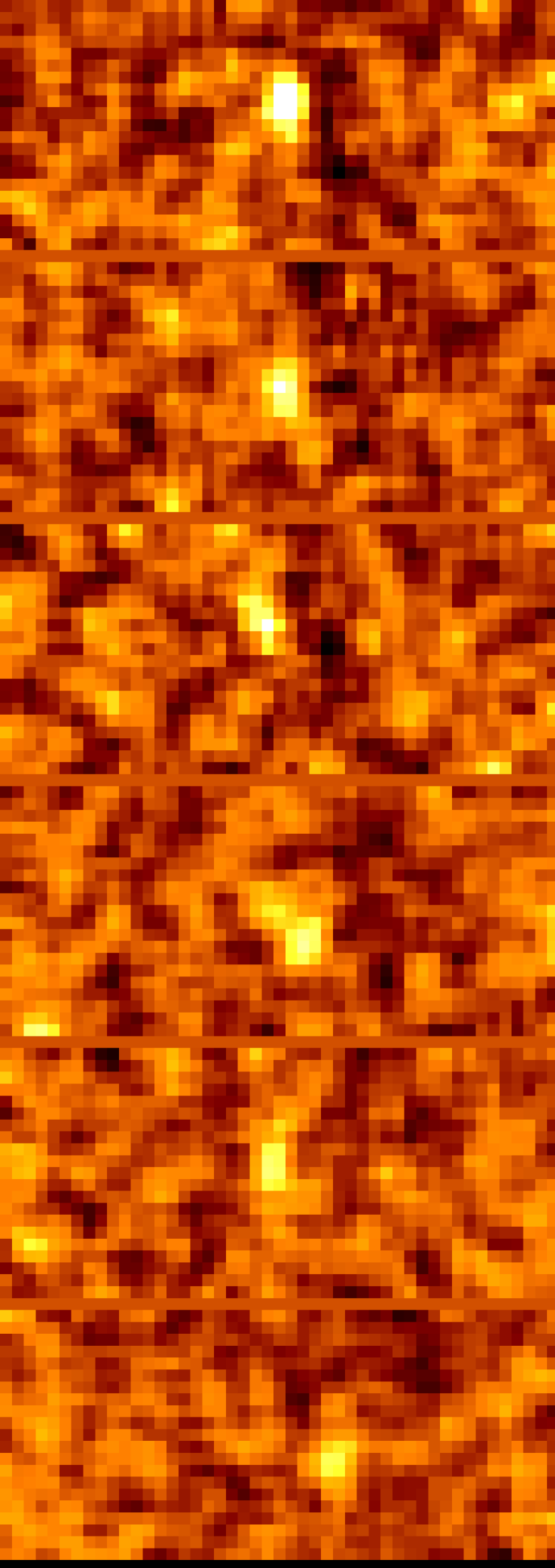
Figure 1: Images of the 2-D spectra of some individual PNe in NGC 1316 . In each image the wavelength direction lies along the horizontal axis, and the spatial direction (i.e. the direction along the slitlet) lies along the vertical axis. Each spectrum shows about 61 Å in wavelength. The spatial extent of the spectra varies but it can be estimated from the pixel scale of $0.26^{\prime\prime}$ per pixel.

Figure 2: The planetary nebulae spatial distribution. The symbol representing each nebula is chosen so that open squares are for velocities approaching and crosses for receding velocities; the symbol size is proportional to the absolute value of the velocity with respect to the systemic velocity. The thick dashed line shows the direction of maximum gradient ($77^{\circ}\pm 28^{\circ}$) found from the linear least-square fit. North is up, and East to the left.

2.2 Absorption line spectra

Long-slit spectra were obtained for NGC 1316  at the Siding Spring Observatory 2.3 meter telescope with the DBS, simultaneously in the blue (4800-5800 Å) and the red (8200-9200 Å) calcium triplet absorption line region. We used 1200 G/mm gratings on both arms of the DBS. The mean dispersion is 0.57 Å pixel^-1 with a velocity resolution of $30\,{\rm\,km\,s^{-1}}$. A Cu-He-Ar lamp was used to wavelength-calibrate the spectra in the blue arm, while a Ne-Ar lamp was used for the red arm of the DBS. The dimensions of the spectra are $1850~{}(\lambda)\times 500$ pixels and the spatial pixel scale is $0.9^{\prime\prime}$ pixel^-1.

Long slit spectra were obtained along the galaxy major and minor photometric axes, at ${\rm P.A.}=50^{\circ}$ and $140^{\circ}$ respectively. Between each 2000s exposure on the galaxy, the telescope was moved to a nearby empty field where a corresponding sky spectrum was acquired, for an accurate subtraction of the sky lines. Calibration exposures were taken after each galaxy and sky frame, and internal quartz-lamp flats were obtained for both arms of the spectrograph. The total exposure time for spectra along ${\rm P.A.}=50^{\circ}$ and $140^{\circ}$ was 1.6 hrs along each ${\rm P.A.}$. Spectra of standard stars, template stars and twilight sky were acquired at the beginning and at the end of the night. The mean seeing during the observations was FWHM =$1.7^{\prime\prime}$. The bias frames showed some transient structures, which did not affect our measurements: bias subtraction was done using the over-scan region at the edge of the CCD frames.

The long slit spectra were bias-subtracted, flat-fielded, and wavelength-calibrated using the corresponding lamp exposures. The same procedure was applied to the sky frames. For the sky subtraction, an averaged sky frame was produced, and the cosmic rays were removed. The sky continuum was fitted with a Legendre polynomial and subtracted off. Then the emission lines in the averaged-continuum subtracted sky frame were normalized to the emission lines in each galaxy spectrum and removed. The resulting spectrum along each ${\rm P.A.}$ was obtained by a median of all sky-subtracted spectra at each ${\rm P.A.}$. The galaxy and template spectra were normalized with respect to the stellar continuum, and the radial velocity and velocity dispersion measurements were obtained using the Fourier correlation quotient method (Bender 1990). The rotation curve and the velocity dispersion profiles are shown in Fig. 3.

Figure 3: Left: mean streaming velocity (lower panel) and velocity dispersion measurements (upper panel) along the projected major (${\rm P.A.}=50^{\circ}$) axis. Right: same quantities for the minor (${\rm P.A.}=140^{\circ}$) axis.

The spectra were filtered with an adaptive filter (Richter et al.  1992), to reduce the noise in the outer regions, and velocities were measured after binning two rows together, to match the seeing conditions during observations. The Calcium triplet data at 8500 Å agree well with the blue data in the inner regions, but do not reach out so far because of the bright sky lines.

2.3 Summary of observational constraints

Images and photometry of NGC 1316  were published by Schweizer (1980), and Caon et al.  (1994). The results of these papers can be summarized as follows. NGC 1316  appears more disturbed than most elliptical galaxies. Prominent shells and plumes point to a recent merger history. There are signs of a substantial dust component in the central region of the galaxy, especially along the minor axis. Inside a major axis distance of $a=1^{\prime}.5$, the image of NGC 1316  is fairly regular, like that of a normal elliptical galaxy. The position angle of the major axis in this region is ${\rm P.A.}\simeq 58^{\circ}$, and the ellipticity is about E3, but the isophote deviations from ellipses are somewhat larger than for normal ellipticals. The effective radii along the major and minor axes are $a_{e}=132^{\prime\prime}$ and $b_{e}=90^{\prime\prime}$ respectively (Caon et al.  1994), so $R_{e}=\sqrt{a_{e}b_{e}}=109^{\prime\prime}$. Between $a=1^{\prime}.5$ and $a=3^{\prime}$, where the bulk of our PN velocities are measured, the major axis position angle is constant at ${\rm P.A.}\simeq 52^{\circ}$. At $a\simeq 3^{\prime}$ we identify the first outer shells, and at that distance from the center a prominent bar or thick disk starts to be visible, at ${\rm P.A.}=60^{\circ}$. At $a=4^{\prime}.5$ the position angle of the major axis is at ${\rm P.A.}\simeq 54^{\circ}$. Fig. 4 reproduces one of Schweizer’s (1980) deep images on which these structures can be seen.

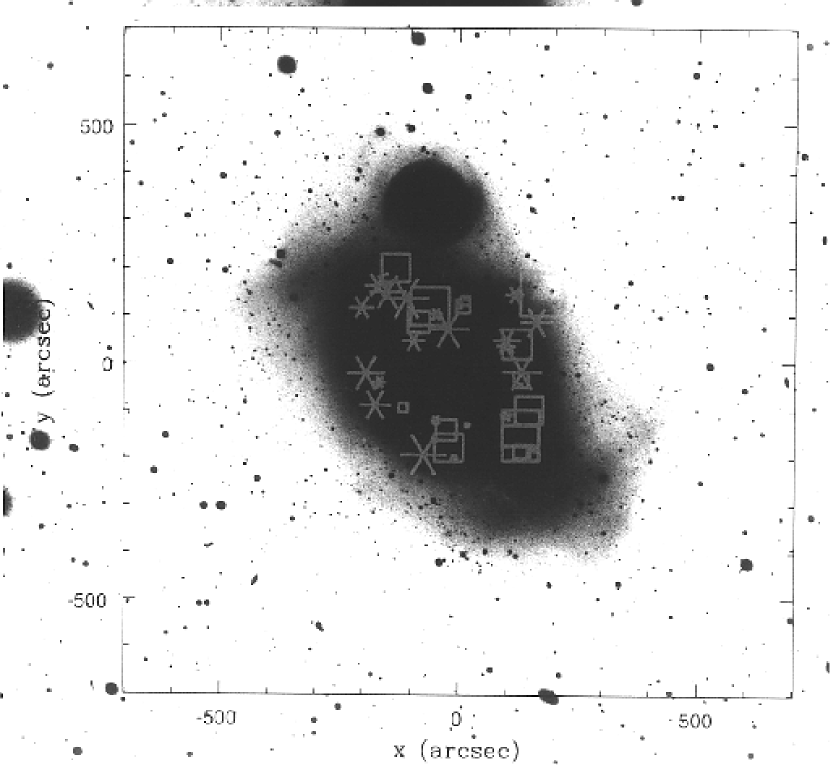
Figure 4: Figure 8 from Schweizer’s 1980 paper, with PNe radial velocity symbols.

Despite the somewhat larger than normal isophote deviations inside $3^{\prime}$, no obvious asymmetry is seen in Schweizer’s images in this inner region. The photoelectrically measured brightness profile of NGC 1316  approximately obeys the $r^{1/4}$ law from about $6^{\prime\prime}$ to at least $6^{\prime}$. This and the approximate constancy of the major axis position angle are consistent with the notion that the gravitational potential of NGC 1316  has largely settled down to a nearly triaxially symmetric configuration, at least inside $3^{\prime}$, but see below.

Is the PN sample representative of the underlying stellar population in the outer region $(r>90^{\prime\prime})$ of NGC 1316 ? The number of PN per unit light in early-type galaxies depends on the integrated B–V of the parent stellar population (Hui et al.  1993). NGC 1316 does not seem to have significant color gradient in its outer parts, where shells, loops and tails become dominant. The photoelectric photometry by Schweizer (1980) indicates a constant value in B–V$\simeq 0.9$ from $18^{\prime\prime}$ to $200^{\prime\prime}$. The aperture photometry from Lauberts & Sadler (1984) reports constant B–V $\simeq 0.9$ out to $300^{\prime\prime}$. More recent results from Schröder & Visvanathan (1996) confirmed a constant color in B–V from $71^{\prime\prime}$ to $142^{\prime\prime}$. The existing multi-color photometry of NGC 1316 is consistent with an homogeneous stellar population for the main spheroid within $300^{\prime\prime}$. Hence we expect the true radial distribution of PN in NGC 1316 to be proportional to the radial distribution of integrated light.

However, the cumulative number density of the observed PN sample does not follow the underlying continuum light, except in the outermost regions. We compared the cumulative number densities of the PNe as well as of the continuum light as a function of surface brightness. They are not linearly related inside $100^{\prime\prime}$, probably due to selection difficulties of faint PNe against the galaxy continuum in the central parts. In the following the PNe must therefore be regarded as a test particle distribution, whose velocity distribution can be regarded as locally representative of the true velocity distribution, but whose density and phase-space density are effectively independent of the true underlying stellar distributions.

The absorption line measurements described in Section 2.2 show that the kinematic major axis is close to the photometric major axis: along ${\rm P.A.}=50^{\circ}$, the radial velocities increase rapidly near the center and then we find a streaming velocity plateau at $a\sim 100^{\prime\prime}$ of $v\simeq 145\,{\rm\,km\,s^{-1}}$, similar to the value found by D’Onofrio et al.  (1995) at $a=50^{\prime\prime}$ for the same ${\rm P.A.}$. Bosma et al.  (1985) find a plateau value of $v\simeq 140-150\,{\rm\,km\,s^{-1}}$ at $80-100^{\prime\prime}$ along ${\rm P.A.}=60^{\circ}$, so the gradients away from ${\rm P.A.}=50^{\circ}-60^{\circ}$ are small. The large rotation along the photometric major axis does not seem to be related to a hidden disk component. Schweizer (1980) ruled out substantial evidence for a disk component brighter than $B\sim 26$, and Caon et al.  (1994) determined the $a_{4}$ parameter of the isophotes inside $2^{\prime}$ to be mostly negative, which is indicative of boxiness.

The absorption line measurements plotted in Figure 3 show that the kinematic minor axis of the stars within $70^{\prime\prime}$ must be near ${\rm P.A.}=140^{\circ}$, close to that of the photometric minor axis: there is no velocity gradient within $30^{\prime\prime}$ of the galaxy nucleus. In this region there is no evidence for a misalignment between photometric and kinematic principal axes in the available absorption line data, and the stellar velocity field is consistent with being axially symmetric. At larger distances along the galaxy minor axis, the radial velocities increase on both sides, producing a U-shape morphology in the radial velocity curve, and the velocity dispersion profile is irregular. This kind of U-shaped velocity morphology is common among interacting ellipticals (Borne et al.  1994), but in these circumstances it lasts for only about one dynamical time. In NGC 1316 the local dynamical time at $40^{\prime\prime}$ is $\sim 3\times 10^{7}{\rm\,yr}$, while from the relaxed morphological appearance inside $3^{\prime}$, the merger cannot have occurred later than $\sim 2\times 10^{8}{\rm\,yr}$ ago. This, and the shape of the NW part of the minor axis velocity curve, suggest that the U-shaped velocity morphology is due to some late–infalling material. If so, the U–shaped velocity curve is associated with a minor perturbation which does not affect the global dynamics. This we will assume in what follows.

3 Analysis of the PN velocity field

In this section we determine the properties of the PN velocity field without reference to the absorption line kinematics. We will first, in Section 3.1, fit a linear velocity field (equivalent to a solid body rotation) and a flat rotation curve to the measured radial velocities. We then investigate non-parametrically whether the direction of maximum rotational gradient obtained from these fits is sensitive to the assumed functional form of the velocity field (Section 3.2).

3.1 Parametric velocity fields

We first make a linear fit to the original sample of 43 radial velocities $v_{rad}(x,y)$ of the form

$$v_{rad}=a_{0}x+a_{1}y+c.$$

Here $x$ and $y$ are pixel coordinates on the CCD frame. $a_{0},a_{1},c$ are determined by a least square fit to the observed radial velocities $v_{rad}$. This linear velocity field is equivalent to solid body rotation of the form

$$v_{rad}=v_{sys}+\omega r\cos(\varphi-\varphi_{0}).$$

where $\varphi$ is the position angle of the PN, $\varphi_{0}$ is the position angle of the kinematic major axis, $r$ is the radius in arcsec, and $v_{sys}$ is the systemic velocity. The origin is the mean $(\bar{x}_{PN},\bar{y}_{PN})$ for the sample. This will give a first indication of whether mean rotation is present in the outer parts of NGC 1316 . This linear fit gives the following parameters: $\bar{x}_{PN}=1212,\,\bar{y}_{PN}=1016,\,v_{sys}=1783\pm 26\,{\rm\,km\,s^{-1}}$ with a maximum gradient of $0.11\pm 0.05\,{\rm\,km\,s^{-1}}$ pixel${}^{-1}=0.42\pm 0.19\,{\rm\,km\,s^{-1}}$ arcsec^-1 along $\varphi_{0}={\rm P.A.}=77^{\circ}\pm 28^{\circ}$ (measured from North towards East). This direction is shown in Fig. 2; along this ${\rm P.A.}$ the mean rotation is $100\pm 45\,{\rm\,km\,s^{-1}}$ at radius of $4^{\prime}=19.7$ kpc. Once this linear component is subtracted from the planetary nebulae radial velocities, the dispersion of the velocity residuals is $170\pm 18\,{\rm\,km\,s^{-1}}$. We note that this value is very similar to the absorption line velocity dispersion of $\sigma\approx 160\,{\rm\,km\,s^{-1}}$ at $60^{\prime\prime}$. The centroid of the PNe resulting from the linear fit is within $7^{\prime\prime}$ of the photometric center of NGC 1316.

We also fitted a flat rotation curve directly to the 43 PN radial velocities, using the following function:

$$v_{rad}=v_{sys}+v_{o}\cos(\varphi-\varphi_{0}).$$

The equations that give the three parameters were solved numerically. The errors on the parameters were computed from the partial variation of $\chi^{2}$ with each parameter. For the flat rotation curve fit, we get the following values for the parameters: $v_{sys}=1783\pm 27\,{\rm\,km\,s^{-1}}$, $\varphi_{0}=70^{\circ}\pm 35^{\circ}$, $v_{0}=67\pm 37\,{\rm\,km\,s^{-1}}$, and the velocity dispersion is $\sigma=175\,{\rm\,km\,s^{-1}}$. The parameters $\varphi_{0},\,v_{0}$ for the flat rotation curve fit are marginally worse determined than $\varphi_{0},\,\omega$ for the solid body rotation fit. The residuals showed no radial trends in either case.

3.2 Non-parametric fitting of the velocity field

In this section we investigate the properties of the 2-D PN velocity field without assuming an “a priori” form for the rotation curve or velocity field. The sample of 43 radial velocities is rather small for fitting a non-parametric velocity field. However, based on the discussion in Section 2.3 we assume that the velocity field is point-symmetric with respect to the center of the galaxy, i.e., that to every velocity $v$ at position $(x,y)$ on the sky there corresponds a velocity $-v$ at position $(-x,-y)$. Such an assumption would be justified both in the case of a general velocity field in a triaxially symmetric potential (resulting in a projected velocity field with minor axis tilt) and for an axisymmetric velocity field (resulting in a bisymmetric projected velocity field without tilt). Assuming point symmetry we construct a sample of 86 data points by reflecting all observed data points around the galaxy center. By fitting a two-dimensional surface to these 86 velocities we derive a smoothed velocity field $\bar{v}(x,y)$.

3.2.1 The smoothing algorithm

We have used the non-parametric smoothing algorithm of Wahba & Wendelberger (1980), originally developed for analyzing meteorological data, to determine the properties of the velocity field $\bar{v}(x,y)$. This algorithm uses thin plate splines to represent a smooth solution $\Phi(\vec{x})$ which minimizes the quantity:

$$\frac{1}{N}\sum_{i=1}^{N}\left[\Phi(\vec{x}_{i})-\Phi_{i}\right]^{2}+\lambda\int_{-\infty}^{\infty}\left(\left[\frac{\partial^{2}\Phi}{\partial x^{2}}\right]^{2}+2\left[\frac{\partial^{2}\Phi}{\partial x\partial y}\right]^{2}+\left[\frac{\partial^{2}\Phi}{\partial y^{2}}\right]^{2}\right)dxdy.$$

Here $N$ is the number of observations $\Phi_{i}$ at positions $\vec{x}_{i}$. The degree of smoothness is controlled by the regularization parameter $\lambda$; in the following, we use $\Lambda=\log(N\lambda)$.

For large values of $\Lambda$, the algorithm in this form will fit a plane through the measured points. For small $\Lambda$ it will minimise deviations between model and data, even at the expense of a noisy model. There will then be a range of $\Lambda$ for which an adequately smooth, non–parametric solution is found which at the same time is a fair representation of the data. For sufficiently good data, the surface from which the data are drawn will be recovered.

The present application is somewhat different from the standard case in that, even for zero observational errors, the measured PNe radial velocities would locally not agree with the fitted velocity field at their positions, due to the galaxy–intrinsic dispersion $\sigma$ in the PNe velocities. In fact, the velocity dispersion dominates over the observational errors. Thus in our case the algorithm will find the best-fitting smooth streaming velocity field by minimising $\sigma$ as much as possible within the imposed smoothness constraints. We therefore need to discuss carefully how the imposed degree of smoothing is chosen.

3.2.2 Determining $\Lambda$.

In the standard case of fitting a function to a sample of measurements drawn from an underlying smooth surface, we can distinguish the following two extreme regimes: (i) For large $\Lambda$ the algorithm would fit a plane through the measured points. If the underlying surface from which the data points are drawn is poorly described by a plane, and the measurement errors are sufficiently small, this would be recognisable in that the mean $\chi^{2}$ per data point with respect to the fitted surface, $<\chi^{2}>$, would be large. (ii) On the other hand, for small values of $\Lambda$ the algorithm would try to fit a very un-smooth velocity field going through all points exactly, with the result that $<\chi^{2}>$ would be much less than one.

A simple way of determining an appropriate value for $\Lambda$ would then be to require that the $<\chi^{2}>$ with respect to the fitted surface should be about unity. For such a value of $\Lambda$ the fitted surface would be consistent with the measurements, within their errors, but it would not be unduly noisy, because the random fluctuations in the measurements around the underlying true values are not followed in detail. In our case, for small $\Lambda$, the algorithm would again try to fit all measured points exactly, except that this is harder because of the large dispersion between neighbouring points. For large $\Lambda$, however, the situation here is different. Since the mean streaming velocity is nowhere larger than the velocity dispersion $\sigma$, even for a velocity field rising non-linearly with $\vec{x}$, $<\chi^{2}>$ could never become much larger than unity. Thus determining $\Lambda$ from the condition that $<\chi^{2}>\simeq 1$, while still possible, would not lead to a very well-determined value of $\Lambda$. Moreover, we have seen above that the 43 measured PN velocities in NGC 1316  are consistent with a nearly linear velocity field. Therefore, since we will want to determine the velocity dispersion $\sigma$ at the same time as the best value for $\Lambda$, we can not use it to fix $\Lambda$.

An often–used procedure to determine the smoothing parameter is the so–called generalised cross validation method (GCV; Wahba & Wendelberger 1980). The idea of cross validation (CV) is to use only $N-1$ rather than $N$ data points to determine the function, ask how well this then predicts the $N^{th}$ measurement, repeat this procedure $N$ times cutting out each of the data points once, evaluate a $<\chi^{2}>$, and choose $\Lambda$ such that this $<\chi^{2}>$ is minimised. GCV is a version of CV that uses a fast approximation for the cross validation function, making the method much easier to apply. In addition, assuming uncorrelated residuals, CV schemes can be used to estimate the mean variance.

Unfortunately, however, GCV gives a robust estimate for $\Lambda$ only when one has at least $\sim 15$ data points with reasonable S/N (in our case, in the dispersion; cf. Wahba & Wendelberger 1980). In fact, we have tried GCV on our small sample, which corresponds to about three such data points, and have found that the method prefers infinite $\Lambda$. This means that GCV cannot distinguish the data from a plane.

Instead we use a Monte–Carlo method to determine $\Lambda$. The idea is to draw artifical data from a known velocity field and see how well one can recover this velocity field from the data in a statistical sense, as a function of $\Lambda$. From the discussion above, one expects the recovered velocity field to deviate from the input field for both small and large $\Lambda$. Both the characteristics of the data and the input velocity field should be as close to the real case as possible.

Thus we construct a characteristic bisymmetric velocity field $v_{\rm in}$, fitting to the observed PNe velocities with $\Lambda=2.2$ (a plausible value). We then draw samples of artifical data from $v_{\rm in}$, and analyse them exactly as we will analyse the observations. Each sample consists of 43 randomly drawn radial velocities at the positions of the observed PNe. The velocity distribution at each position is a Gaussian with dispersion $\sigma=165{\rm\,km\,s^{-1}}$ centered on $v_{\rm in}$. Then, for a range of values of $\Lambda$, we determine the line of maximum gradient as described in section 3.2.3, and fit a bisymmetric velocity field $v_{\rm MC,\Lambda}$ to the 172 bi–symmetrized artificial data points, using the particular $\Lambda$ and the line of maximum gradient obtained with this $\Lambda$. On a grid in ($x,y$) we finally determine the quantity $\chi_{\rm MC,\Lambda}^{2}=[v_{\rm MC,\Lambda}-v_{\rm in}]^{2}$, which gives the average quadratic deviation of the velocity field determined by the data, from the velocity field from which the data were drawn. Repeating this for a large number of Monte Carlo samples results in a smooth average $\chi_{\rm MC}^{2}(\Lambda)$, which should have a minimum at a certain value of $\Lambda$. In a statistical sense, a sample of 43 PNe is best analyzed with this optimal $\Lambda$, and therefore this value should be used in the fitting algorithm.

Fig. 5 shows $\chi_{\rm MC}^{2}(\Lambda)$ (solid line) for 450 samples of 43 velocities each, drawn from $v_{\rm in}$. As expected, small values of $\Lambda$ lead to large errors in the reconstruction of $v_{\rm in}$, due to amplified noise. However, because of the near–linearity of $v_{\rm in}$, the small number of observed radial velocities, and the large ratio of dispersion to rotation velocity, no increase towards large $\Lambda$ is visible. For $\Lambda\mathrel{\hbox to0.0pt{\lower 3.0pt\hbox{$\mathchar 536\relax$}\hss}\raise 2.0pt\hbox{$\mathchar 318\relax$}}2$, $\chi_{\rm MC}^{2}(\Lambda)$ is nearly constant which means that with 43 velocities and $\sigma=165{\rm\,km\,s^{-1}}$ it is not possible to distiguish $v_{\rm in}$ from a planar velocity field – all velocity fields obtained for $\Lambda\mathrel{\hbox to0.0pt{\lower 3.0pt\hbox{$\mathchar 536\relax$}\hss}\raise 2.0pt\hbox{$\mathchar 318\relax$}}2$ are equally plausible. The same is true for a cylindrical velocity field with more spatial structure, drawn from an arctan-function: then also no minimum is found (short dashed line). However, increasing the number of points to 100 in this case results in a clear minimum (long dashed line). In the following, we use as a plausible value for the smoothing parameter the smallest $\Lambda$ for which $\chi_{\rm MC}^{2}(\Lambda)$ has not increased significantly, i.e., $\Lambda=2.2$. This ensures that the regularisation suppresses as little structure in the velocity field as possible, while at the same time the small number of data points is not overinterpreted.

Figure 5: Average deviation $\chi_{\rm MC}^{2}(\Lambda)$ of an inferred bisymmetric velocity field from the input velocity field $v_{\rm in}$, as a function of $\Lambda$. The solid curve shows the results for a field $v_{\rm in}$ determined from the 43 observed PNe velocities using $\Lambda=2.2$ and a velocity dispersion of $\sigma=165{\rm\,km\,s^{-1}}$. The short–dashed line is for 43 PNe drawn at random positions from an $\arctan$ velocity field with the same dispersion. The long–dashed line is for the same $v_{\rm in}$, but with a sample of 100 PNe. A clear minimum is visible only for 100 data points.

The smoothed velocity field $\bar{v}(x,y)$ obtained by fitting a two-dimensional surface to the velocities of the point-symmetric PN radial velocity sample is shown in Fig. 6. Fig. 7 shows the residual velocity distribution for this case. The width $(\Delta v)_{{\caps rms}}=165\,{\rm\,km\,s^{-1}}$ of this distribution is our best estimate for the PN velocity dispersion $\sigma$.

3.2.3 Determining the direction of maximum rotational gradient

Now we derive the properties of the velocity field $\bar{v}(x,y)$. We first want to determine the angle $\varphi$ for the direction of maximum gradient, independent of the functional form adopted for the velocity field. To this end, for any value of $\varphi$ in the range $[0,180]$ degrees,

(1) we symmetrize the 86 velocity data points around an axis which is rotated by $\varphi$ with respect to the $x$-axis of the CCD frame (centered on NGC 1316 ). From the set of 86 data points we thus obtain 172 data points. If $x_{PN},y_{PN}$ are the PN coordinates in the CCD frame, the symmetric data points are derived from the measured PN coordinates as follows:

$$x^{\prime}_{PN}=x_{PN}\cos\varphi+y_{PN}\sin\varphi \rightarrow x^{\prime}_{\rm sym}=x^{\prime}_{PN}$$

$$y^{\prime}_{PN}=-x_{PN}\sin\varphi+y_{PN}\cos\varphi \rightarrow y^{\prime}_{\rm sym}=-y^{\prime}_{PN}$$

$$v^{\prime}_{\rm rad}=v_{\rm rad} \rightarrow v^{\prime}_{\rm sym}=-v^{\prime}_{\rm rad}$$

(2) we fit a bisymmetric velocity field $\bar{v}_{2}(x^{\prime},y^{\prime}|\varphi)$ to these 172 symmetrized data points, using the Wahba & Wendelberger algorithm and a smoothing parameter $\Lambda=2.2$.

Then we determine $\varphi$ by minimising $\chi^{2}\equiv[\bar{v}_{2}(x^{\prime},y^{\prime}|\varphi)-\bar{v}(x,y)]^{2}$ on a grid in the $(x^{\prime},y^{\prime})$–plane. This results in the best bisymmetric approximation to the original velocity field $\bar{v}(x,y)$. Fig. 8 shows $\chi^{2}=[\bar{v}_{2}(x^{\prime},y^{\prime}|\varphi)-\bar{v}(x,y)]^{2}$ as a function of $\varphi$. Note that there is a distinct minimum at $\varphi_{\rm min}=80^{\circ}$, at which the rms deviation between the two smoothed velocity fields $\bar{v}(x,y)$ and $\bar{v}_{2}(x^{\prime},y^{\prime}|\varphi)$ is $6\,{\rm\,km\,s^{-1}}$. Thus at the high level of smoothing required by the small number of PN velocities, the smoothed velocity field $\bar{v}$ is consistent with four–fold symmetry. There is no significant dependence of $\varphi_{\rm min}$ on $\Lambda$; even in the case of the noisy velocity fields obtained for $\Lambda\simeq 1.5$ the best $\varphi$ differs from $\varphi_{\rm min}$ only by $\sim 10^{\circ}$. The fact that the minimum is well determined implies that there is a significant direction of maximum gradient.

We determine an error on $\varphi_{\rm min}$ in two ways. First, we compute the likelihood of the 43 measured PN velocities, given a velocity field $\bar{v}_{2}(x,y|\varphi)$:

$$\log P_{\rm PN}(\varphi)=-\sum_{i}(\bar{v}_{2}(x,y|\varphi)-v_{i})^{2}/2\sigma^{2}+{\rm const.,}$$

where the position and radial velocity of planetary nebula $i$ are denoted by $x_{i}$, $y_{i}$, $v_{i}$, and the velocity dispersion is $\sigma=165\,{\rm\,km\,s^{-1}}$, as determined for $\Lambda=2.2$ and consistent with the absorption line velocities in Fig. 3. The relative likelihood $P_{\rm PN}(\varphi)/\mbox{max}P_{\rm PN}(\varphi)$ is plotted in Fig. 8. Relative to the maximum likelihood value of $\varphi=76^{\circ}$, the function has decreased to $\exp(-1/2)$ at $\varphi=(109^{\circ},48^{\circ})$. Second, we have determined the distribution of $\varphi_{\rm min}$ for a set of Monte Carlo generated data sets of 43 data points each, drawn from the point–symmetric velocity field $\bar{v}(x,y)$. This has a maximum at $\varphi_{\rm min}=81^{\circ}$ with a dispersion of $30^{\circ}$. Both estimates of the error are consistent. From the non-parametric fit of the 43 PNe radial velocity sample, we conclude that the line of maximum gradient for the PN data (hereafter LOMG) is $\varphi=80^{\circ}\pm 30^{\circ}$. This inferred direction is in good agreement with the ${\rm P.A.}$ determined via the parametric function fitting.

3.2.4 Properties of the velocity field

Fig. 6 shows the derived PN velocity field rotated such that the $x$-axis lies along the LOMG at $\varphi=80^{\circ}$. For comparison, we also show the bisymmetric velocity field $\bar{v}_{2}(x^{\prime},y^{\prime}|\varphi)$; the difference between these is not significant (rms $6\,{\rm\,km\,s^{-1}}$). The rotation of about $140\,{\rm\,km\,s^{-1}}$ at $4^{\prime}$ is clearly apparent.

The residual velocity distribution about this velocity field is nearly Gaussian, as already shown in Fig. 7. The value of $\chi^{2}=[\bar{v}_{2}(x^{\prime},y^{\prime}|80^{\circ})-v_{\rm rad}]^{2}=2.73\times 10^{4}({\rm\,km\,s^{-1}})^{2}$ which gives a $\sigma_{PN}=165\,{\rm\,km\,s^{-1}}$ after the mean streaming velocity field is accounted for. This is similar to the values derived from the parametric fits.

For our best value of $\varphi_{\rm min}=80^{\circ}$, we project the point symmetric data set of 86 points onto the LOMG, and then compute a smoothed rotation curve via Wahba & Wendelberger’s smoothing algorithm. For small $\Lambda$, the resulting rotation curve shows substantial counter-rotation in the central parts, which is excluded by the absorption line data and must therefore be an artifact of the small number of PN velocities in the sample. Thus we take for $\Lambda$ the minimum value for which we do not have counter rotation in the central region ($\Lambda=4$). By choosing $\Lambda$ in this way, we also smooth away some real velocity gradient in the outer parts.

Fig. 9 shows the smoothed rotation curves so derived along the LOMG ($\varphi=80^{\circ}$) and the perpendicular direction ($\varphi=170^{\circ}$). No significant rotation is seen along the perpendicular axis. Along the LOMG there is clear rotation in the outer parts and we obtain a rotation of $140\pm 60\,{\rm\,km\,s^{-1}}(1\sigma)$ at $4^{\prime}=19.7$ kpc. It is not clear whether we have rotation in the inner parts. This is because the PNe sample lacks objects at small distances from the galaxy center, and the radial velocities of PNe which appear at small projected distances from the center in Fig. 9 actually sample the gravitational potential high above the major axis. Therefore the mean velocity curve shown in the top left panel of Fig. 9 really provides no information about rotation at radii less than $80^{\prime\prime}$ from the center. In the next section, we will use the absorption line data to fill in this gap.

We next divide the PN velocity points into two about equal subsamples: those points whose $y^{\prime}<121.5^{\prime\prime}=9.8$ kpc from the LOMG, and those for which $y^{\prime}>121.5^{\prime\prime}$. We project both sets of velocities independently onto the LOMG and fit a rotation curve to each set separately with the same $\Lambda=4$. Fig. 9 shows at best a hint of the PNe with $y^{\prime}<121.5^{\prime\prime}$ rotating faster at the larger radii ( $179\,{\rm\,km\,s^{-1}}$ at 18.5 kpc ) than those with $y^{\prime}>121.5^{\prime\prime}$. The fast rotation signal at large major axis radius near the plane comes from PNe on both sides of the center. The difference between both subsamples is only $\simeq 0.5\sigma$. Also, if we fit a linear rotation curve to both subsets of the data, the derived slopes are nearly identical. Thus any non-cylindrical rotation needs to be confirmed with a larger sample of PN velocities.

Inspection of Fig. 4 reproduced from Schweizer (1980) shows an elongated bar-like or thick disk structure at a distance of $\sim 3^{\prime}$ from the center of NGC 1316  along a ${\rm P.A.}=60^{\circ}$. The large rotation velocity in the outer parts inferred from the PN velocities might reflect rotation connected with this structure, which is within $1\,\sigma$ of the ${\rm P.A.}$ of the LOMG. This is a similar situation to the outer region of Cen A, NGC 5128, where the outer PNe with high rotation and small $\sigma$ are associated with an elongated light distribution.

Figure 6: Left panel: smoothed point-symmetric velocity field $\bar{v}(x^{\prime},y^{\prime})$ for $\Lambda=2.2$, rotated to coordinates where the $x^{\prime}$–axis is at position angle $\varphi=80^{\circ}$. Right panel: four–fold symmetric velocity field $\bar{v}_{2}(x^{\prime},y^{\prime}|\varphi)$ for the optimal major–axis direction $\varphi_{\rm min}=80^{\circ}$ and $\Lambda=2.2$. The contours are spaced by $\Delta v=22.7~{}{\rm\,km\,s^{-1}}$, decreasing from left to right, and the central contour has $v=9~{}{\rm\,km\,s^{-1}}$.

Figure 7: The distribution of residual velocities from the fitted velocity field $\bar{v}$ for $\Lambda=2.2$ (solid line) and a Gaussian velocity distribution with the same dispersion $\sigma=165\,{\rm\,km\,s^{-1}}$ (dotted line). The bin size is $100\,{\rm\,km\,s^{-1}}$.

Figure 8: Top: $\chi^{2}=(\bar{v}_{2}(x^{\prime},y^{\prime}|\varphi)-\bar{v}(x,y))^{2}$ as a function of $\varphi$. Bottom: relative likelihood of the measured PN velocities for $\bar{v}_{2}(x^{\prime},y^{\prime}|\varphi)$ as a function of $\varphi$.

Figure 9: Smoothed rotation curves from PN velocities. Top left: along the LOMG, for the point symmetric data set 86 velocities (with $\Lambda=4$). Different symbols are used to identify the actually observed 43 points (open circles), and their symmetric counterpart (stars). Bottom left: same, along the axis orthogonal to the LOMG. Top right: along the LOMG, but only for data points at heights less than $121.5^{\prime\prime}$ above the LOMG. Bottom right: same, but only for data points at heights larger than $121.5^{\prime\prime}$ above the LOMG. In each panel the full line is obtained with $\Lambda=4$, the dashed line shows the linear fit from Section 3.1. The squares and thick error bars indicate the mean velocity and its error, the thin “error bars” the calculated velocity dispersion $\sigma$, all computed in a small number of bins each containing about one fifth of the PNe. The $1\sigma$ error on the mean velocity is given by the velocity dispersion divided by $\sqrt{N_{\rm bin}}$, i.e., about $60{\rm\,km\,s^{-1}}$, making the outermost rotation a $2.3\sigma$ result.

4 Combined velocity field from PNe and absorption line data

The PNe provide us with little information about the rotation near the center of the system. We therefore now construct a velocity field using the integrated light spectroscopy in the inner regions and the PNe velocities in the outer regions. Fig. 10 shows the combined data with the PNe reflected about the adopted minor axis of the absorption line data, reversing their sign in velocity when reflected.

To the combined data, we fit a velocity field using the smoothing algorithm, with $\Lambda=1.2$ to resolve the stronger curvature in the absorption line data. Here the relative weights of the PN absorption data and the PNe were chosen according to their measurement errors. The error for the PNe velocities is $60{\rm\,km\,s^{-1}}$; the errors for the absorption line data are shown in Fig. 3. Where there are absorption line velocities, they essentially fix the fitted curve; where there are none they only enter through the regularisation. The PNe fix the curve far from where absorption line data exist, but have almost no effect in regions where the absorption line data dominate. Giving the PNe data additionally different weights results in a very similar curve when $\Lambda$ is changed according to the new weights.

We have argued earlier that the minor axis velocities are influenced by non–equilibrium effects. We have therefore constructed velocity fields both with and without the minor axis data. The essential features of the velocity field including the minor axis data (left panel of Fig. 11) and that without (right panel) are closely similar. A velocity peak at $60^{\prime\prime}$ corresponds to the maximum value of the rotation curve reached in the integrated light measurements, see Fig. 3; a second peak at $\sim 200^{\prime\prime}$ corresponds to the PNe rotation of $140\,{\rm\,km\,s^{-1}}$ found at $4^{\prime}$ in Section 3. The dip between the two peaks is approximately $35\,{\rm\,km\,s^{-1}}$ below the peaks while we estimate that the error on the velocities of these major features is about $60\,{\rm\,km\,s^{-1}}$. Thus the dip is hardly significant. In gross terms, the velocity field in Fig. 11 is similar to the velocity field plotted in Fig. 5 of Dehnen & Gerhard (1994) for a rotating isotropic oblate $\gamma=3/2$ model. This velocity field does not have rotation along the minor axis.

Fig. 12 shows the combined data projected onto the photometric major axis at ${\rm P.A.}=50^{\circ}$ and minor axis at ${\rm P.A.}=140^{\circ}$ in much the same way as Fig. 9 for the PNe alone. Because the photometric major axis is misaligned with respect to the LOMG for the PNe sample, the PN rotation velocities at several arcmin radius in Fig. 12 are noticeably smaller than those in Fig. 9. The difference is about $1\sigma$, similar to the significance of the misalignment. The fitted mean rotation curves are clearly dominated by the absorption line data in the region where these are available. Especially from the top right panel of Fig. 12, which plots the absorption line data and the lower half of the PNe data within $73^{\prime\prime}$ of the major axis, it appears that the PNe are not drawn from the absorption line velocity curve. Probably this is because even the lower half of the PNe distribution samples a different part of the velocity field than does the major axis absorption line data. In other words, the gradients in $z$ must be relatively strong.

It is not possible to recover the dependence of the velocity dispersion on radius nonparametrically with a small sample like ours. To check whether the velocity dispersion changes with radius at all, we divide the PN data into two bins in major axis radius and determine the rms velocity dispersion with respect to the rotation curve shown in Fig. 12. We calculate the variance of the residual velocities both for the full PNe sample and for the lower half of the sample close to the major axis.

Fig. 13 shows the mean rotation velocity and velocity dispersion along the major axis from the absorption line data and from the binned PNe data. The lower panel of Fig. 13 shows a spherically averaged velocity curve, giving major axis and minor axis $\sqrt{v^{2}+\sigma^{2}}$ for the absorption line data, and binned values of $\sum_{i}(v_{i}-v_{\rm sys})^{2}$ for the PNe.

The total variance with respect to the fitted rotation velocity includes the measurement error $\sigma_{\rm obs}=42\,{\rm\,km\,s^{-1}}$ and the intrinsic velocity dispersion $\sigma_{\rm int}$ in the galaxy, where $\sigma^{2}=\sigma_{\rm obs}^{2}+\sigma_{\rm int}^{2}$. For a variance of $\sigma=165\pm 17\,{\rm\,km\,s^{-1}}$ this results in an intrinsic velocity dispersion of $\sigma_{\rm int}=159\pm 17\,{\rm\,km\,s^{-1}}$. The error $\delta\sigma_{\rm int}$ is calculated as the variance of the $\chi^{2}$–distribution and is given by $\delta\sigma_{\rm int}=\sigma_{\rm int}/\sqrt{2(N-1)}$ with $N$ the size of the sample and $N-1$ the number of degrees of freedom. The PNe dispersions plotted in Fig. 13 are the galaxy–intrinsic velocity dispersions $\sigma_{\rm int}$.

Within the error bars, the major axis rotation velocity outside $50^{\prime\prime}$ is constant at $v=110\,{\rm\,km\,s^{-1}}$, the major axis dispersion outside $50^{\prime\prime}$ (the central peak) is constant at $150\,{\rm\,km\,s^{-1}}$, and the spherically averaged mean squared velocity outside $40^{\prime\prime}$ is constant at $v=200\,{\rm\,km\,s^{-1}}$.

Figure 10: Rotation velocities in the combined data. The densely packed points along $y=0$ represent the major axis rotation velocities from the integrated light data along ${\rm P.A.}=50^{\circ}$. Those along $x=0$ represent the minor axis velocities along ${\rm P.A.}=140^{\circ}$. The isolated symbols show the velocities for the individual PNe. Those at negative major axis coordinate $x$ have been reflected about ${\rm P.A.}=140^{\circ}$ and their velocities reversed. The coding is the same as in Fig. 2 (open squares are for velocities approaching, size of the symbol proportional to absolute velocity).

Figure 11: Velocity field derived from the absorption line data combined with the PNe data symmetrized around both major and minor axes. The thin contours are spaced by $16.6~{}{\rm\,km\,s^{-1}}$, starting at central $9.5~{}{\rm\,km\,s^{-1}}$; thick contours are at zero. The left panel shows the velocity field including the minor axis absorption line velocities; the right panel without. Both have been constructed with the smoothing algorithm and $\Lambda=1.2$ (see Section 3). In both panels there are thus 86 velocity points fitted in the region shown, but the fit was actually done between $-250^{\prime\prime}$ and $250^{\prime\prime}$ for all 172 points together with the unaltered respective absorption line data. This ensures that in the right panel the velocities on the minor axis would be zero.

Figure 12: Smoothed rotation curves (full lines) obtained from absorption line data and PN velocities, with $\Lambda=4$. Top left: along ${\rm P.A.}=50^{\circ}$, the photometric major axis. The entire point symmetric data set of 86 PN velocities was used, with different symbols to identify the actually observed 43 points (open circles), and their symmetric counterpart (stars). Bottom left: same, along the photometric minor axis. Top right: along the major axis, but only absorption line velocities and PNe data points at heights less than $73^{\prime\prime}$ above the major axis. Bottom right: same, but only for PNe data points at heights larger than $73^{\prime\prime}$ above the photometric major axis. There are no absorption line data at these heights. The squares and thick error bars in each panel indicate the mean velocity and its error, the thin “error bars” the calculated velocity dispersion $\sigma$, all computed in a small number of bins each containing about one fifth of the PNe. The $1\sigma$ error on the mean velocity is given by the velocity dispersion divided by $\sqrt{N_{\rm bin}}$, i.e., about $60\,{\rm\,km\,s^{-1}}$.

Figure 13: Mean rotation velocity and velocity dispersion as a function of distance, from absorption and PNe data. Top panel: rotation velocity as a function of major axis radius $R$. Curve is taken from Fig. 12, top left, the two outer points are computed from the PNe velocities ordered in $R$ and binned in equal halves. Middle panel: velocity dispersion as function of $R$. The outer points with larger error bars show the dispersion around the mean rotation velocity of the PN sample in two bins (standard deviation). Filled squares in both panels are obtained from Fig. 12, top left, open squares from Fig. 12, top right (half of the sample closer to the major axis). Bottom panel: mean square absorption line velocities $\sqrt{v^{2}+\sigma^{2}}$ on the major axis, rescaled to equivalent spherical radius by $r=\sqrt{0.7}R$ (filled circles). Same for minor axis absorption line velocities, rescaled to equivalent spherical radius by $r=R/\sqrt{0.7}$ (open circles). Full squares show equivalent spherical PNe velocity dispersions $(\sum(v_{i}-v_{\rm sys})^{2}/(N_{\rm bin}-1))^{1/2}$ in two bins. Bin radii are mean values of $\sqrt{q(x_{i}^{2}+y_{i}^{2}/q^{2})}$ for the respective halves of the sample.

5 Dynamics and Mass Estimates

From the measured kinematics we can now estimate the dynamical support by rotation. We do this in two ways. First, we evaluate

$$\left(v\over\sigma\right)^{\ast}\equiv{v_{\rm max}\over\overline{\sigma}}/\sqrt{\epsilon\over 1-\epsilon}$$

(Kormendy 1982). Here $v_{\rm max}$ and $\overline{\sigma}$ are the maximum observed rotation velocity and the luminosity–weighted mean of the major axis dispersion inside $0.5a_{e}$, and $\epsilon$ the observed ellipticity. From Fig. 3 we estimate $v_{\rm max}=145{\rm\,km\,s^{-1}}$ and $\overline{\sigma}=185{\rm\,km\,s^{-1}}$, whereas the mean ellipticity within $a_{e}/2$ is $\epsilon\simeq 0.37$ (Schweizer 1980, Caon et al. 1994). We thus find $(v/\sigma)^{\ast}=1.02$. This is somewhat smaller than the corresponding value obtained for isotropic rotator models ($(v/\sigma)^{\ast}\mathrel{\hbox to0.0pt{\lower 3.0pt\hbox{$\mathchar 536\relax$}\hss}\raise 2.0pt\hbox{$\mathchar 318\relax$}}1.2$; Dehnen & Gerhard 1994), but shows that rotation is dynamically important.

Secondly, we use mass–weighted velocities from the kinematic data in Fig. 13 outside $50^{\prime\prime}$. For the mass–weighted projected rotation velocity we take $\tilde{v}=110{\rm\,km\,s^{-1}}$, and for the projected dispersion $\tilde{\sigma}=150{\rm\,km\,s^{-1}}$, giving $\tilde{v}/\tilde{\sigma}=0.73$. The predicted value for an oblate isotropic spheroid seen edge–on, using a projection factor of $\pi/4$ derived by Binney (1978), is evaluated from equation (5.8) of Gerhard (1994):

$${\tilde{v}\over\tilde{\sigma}}\simeq{\pi\over 4}\sqrt{2\left[(1-\epsilon)^{-0.9}-1\right]}.$$

With an average ellipticity of $\epsilon=0.3$ in the range of radii considered (Caon et al. 1994), this gives $\tilde{v}/\tilde{\sigma}=0.68$, i.e., $(\tilde{v}/\tilde{\sigma})^{\ast}=1.07$. Thus the main body of NGC 1316 is consistent with an isotropic rotator with $\epsilon=0.3$ (inclination effects on this conclusion are weak, Binney 1978).

We will now estimate the mass of NGC 1316 assuming that the galaxy is near–edge on and isotropic. The Jeans equation in the equatorial plane $z=0$ of an axisymmetric system in cylindrical coordinates reads

$$\left(\mathchoice{\partial\Phi\over\partial R}{\partial\Phi/\partial R}{\partial\Phi\over\partial R}{\partial\Phi\over\partial R}\right)_{z=0}={{\bar{v}_{\phi}}^{2}\over R}-{\sigma_{R}^{2}\over R}\left[\mathchoice{\partial\ln\rho\over\partial\ln R}{\partial\ln\rho/\partial\ln R}{\partial\ln\rho\over\partial\ln R}{\partial\ln\rho\over\partial\ln R}+\mathchoice{\partial\ln\sigma_{R}^{2}\over\partial\ln R}{\partial\ln\sigma_{R}^{2}/\partial\ln R}{\partial\ln\sigma_{R}^{2}\over\partial\ln R}{\partial\ln\sigma_{R}^{2}\over\partial\ln R}+1-{\sigma_{\phi}^{2}\over\sigma_{R}^{2}}+{R\over\sigma_{R}^{2}}\mathchoice{\partial\overline{v_{R}v_{z}}\over\partial z}{\partial\overline{v_{R}v_{z}}/\partial z}{\partial\overline{v_{R}v_{z}}\over\partial z}{\partial\overline{v_{R}v_{z}}\over\partial z}\right]_{z=0}.$$ (1)

Here ${\bar{v}_{\phi}}$ is the intrinsic rotational streaming velocity, $\sigma_{R}$ and $\sigma_{\phi}$ are the radial and azimuthal velocity dispersions, $\rho$ is the density, all referring to an equilibrium tracer population that need not be self-consistent with the potential, and $\Phi$ is the total gravitational potential. The PNe are not an equilibrium distribution even if they emerge from an equilibrium distribution of stars because of the selection effects; therefore they are only used as tracers of the underlying velocity field. The last derivative term depends on the orientation of the stellar velocity ellipsoid. This term vanishes for a flattened system with velocities isotropic in the meridional plane. The equatorial potential gradient may be associated with a ‘mass’ $M_{\rm eq}(R)=R^{2}(\mathchoice{\partial\Phi\over\partial R}{\partial\Phi/\partial R}{\partial\Phi\over\partial R}{\partial\Phi\over\partial R})_{z=0}/G$, which overestimates the real mass within $R$ by a factor of order unity except in the case where the potential is spherical. For a spheroidal density distribution with flattening $\epsilon=0.3$ and a density profile inversely proportional to the elliptical radius squared, this factor is $f_{0.3}=1.13$.

To apply this equation, we again set the projected rotation velocity $v=(\pi/4)v_{\phi}$. Isotropy implies $\sigma=\sigma_{R}=\sigma_{\phi}$, and since the velocity dispersion profile is approximately flat, only the first term in the square bracket survives. At a radius of $200^{\prime\prime}=16\,{\rm\,kpc}=1.5a_{e}$ on the major axis the logarithmic slope of the density profile for a de Vaucouleurs model is $\simeq-2.9$, so the equatorial mass is $f_{0.3}^{-1}\times M_{\rm eq}(200^{\prime\prime})=2.9\times 10^{11}{\rm\,M_{\odot}}$.

A similar estimate can be obtained from the spherical Jeans equation

$$M(r)=-{r\sigma_{r}^{2}\over G}\left(\mathchoice{\hbox{d}\ln\rho\over\hbox{d}\ln r}{\hbox{d}\ln\rho/\hbox{d}\ln r}{\hbox{\sevenrm d}\ln\rho\over\hbox{\sevenrm d}\ln r}{\hbox{\fiverm d}\ln\rho\over\hbox{\fiverm d}\ln r}+\mathchoice{\hbox{d}\ln\sigma_{r}^{2}\over\hbox{d}\ln r}{\hbox{d}\ln\sigma_{r}^{2}/\hbox{d}\ln r}{\hbox{\sevenrm d}\ln\sigma_{r}^{2}\over\hbox{\sevenrm d}\ln r}{\hbox{\fiverm d}\ln\sigma_{r}^{2}\over\hbox{\fiverm d}\ln r}+2\beta\right)$$

and the results in the bottom panels of Fig. 13. Here $\sigma_{r}(r)$ is the radial velocity dispersion, and $\beta(r)\equiv 1-\sigma_{\phi}^{2}/\sigma_{r}^{2}<1$ the anisotropy parameter. Assuming again isotropy we have $\beta=0$, and, since the outer rotation velocity field is not cylindrical, $\sigma=150{\rm\,km\,s^{-1}}\mathrel{\hbox to0.0pt{\lower 3.0pt\hbox{$\mathchar 536\relax$}\hss}\raise 2.0pt\hbox{$\mathchar 316\relax$}}\sigma_{r}\mathrel{\hbox to0.0pt{\lower 3.0pt\hbox{$\mathchar 536\relax$}\hss}\raise 2.0pt\hbox{$\mathchar 316\relax$}}\sqrt{v^{2}+\sigma^{2}}=200{\rm\,km\,s^{-1}}$, approximately independent of $r$. Then we find $2.4\times 10^{11}{\rm\,M_{\odot}}\mathrel{\hbox to0.0pt{\lower 3.0pt\hbox{$\mathchar 536\relax$}\hss}\raise 2.0pt\hbox{$\mathchar 316\relax$}}M(200^{\prime\prime})\mathrel{\hbox to0.0pt{\lower 3.0pt\hbox{$\mathchar 536\relax$}\hss}\raise 2.0pt\hbox{$\mathchar 316\relax$}}4.3\times 10^{11}{\rm\,M_{\odot}}$. A modest radial anisotropy in the outer regions of NGC 1316, such as inferred from modelling the line profiles in NGC 2434 (Rix et al. 1997), NGC 6703 (Gerhard et al. 1998) and NGC 1600 (Matthias & Gerhard 1998) would increase both estimates somewhat.

We do not have our own B-band photometry for NGC 1316 , so we will use published photometry for estimating the M/L ratio inside a radius $R=200^{\prime\prime}$. If we compute the integrated luminosity inside $200^{\prime\prime}$ using the aperture photometry listed in Lauberts & Sadler (1984), we obtain $L_{B}=3.7\times 10^{10}L_{\odot}$ which implies a M/L_B ratio of $7.7$. To test for a gradient in the mass–to–light ratio, we similarly compute integrated luminosities and masses interior to radii $45^{\prime\prime},\,90^{\prime\prime},\,143^{\prime\prime}$. Masses are computed again from eq. 1 with the same assumptions as before; these are only applicable outside $\sim 50^{\prime\prime}$. We obtain masses $4.9\times 10^{10}{\rm\,M_{\odot}}$, $1.1\times 10^{11}{\rm\,M_{\odot}}$, $1.8\times 10^{11}{\rm\,M_{\odot}}$ inside these radii, and cumulative mass–to–light ratios of 4.3, 5, 6.4, respectively, compared to a value of 7.7 at $200^{\prime\prime}$.

NGC 1316 and Cen A have somewhat similar morphological properties: Figure 14 shows that their radial distributions of M/L_B, as estimated from PN velocities in the same range of radius, are strikingly similar (see Hui et al.  1995 for the Cen A data). We note that the adopted distances for these two galaxies are on the same system (planetary nebulae luminosity function and surface brightness fluctuations). The apparent radial increase of M/L in these two systems follows from (i) the observed $r^{1/4}$ or Hernquist distributions of surface brightness, (ii) the observed approximate constancy of $\sigma^{2}+v^{2}$ with radius, and (iii) the assumption of isotropy at all radii: this assumption may not be correct, so the precise shape of the M/L$(r)$ relation is still somewhat uncertain. Nevertheless, the similarity of the M/L scale for these two galaxies is remarkable.

Figure 14: The dashed line indicates the M/L_B ratio as function of radius for NGC 5128; triangles indicates the M/L_B ratios obtained for NGC 1316 at $R=45^{\prime\prime},\,90^{\prime\prime},\,143^{\prime\prime},\,200^{\prime\prime}$.

6 Conclusions

The planetary nebulae  radial velocities show the presence of rotation in the outer parts of NGC 1316 , in the direction of an elongated structure visible in Schweizer’s deep image of this galaxy. This elongated structure is orthogonal to the inner minor axis dust lane. The mean rotation velocity along the galaxy’s photometric major axis is constant outside $50^{\prime\prime}$ at $v=110{\rm\,km\,s^{-1}}$, out to the maximum observed radius of $200^{\prime\prime}=1.8R_{e}=16$  kpc. Based on combined integrated light data in the central regions plus PNe radial velocity data in the galaxy’s halo the velocity dispersion profile along the galaxy major axis is consistent with being flat at $150{\rm\,km\,s^{-1}}$ between 4  kpc and 16  kpc.

From the Jeans equations and the assumption of isotropy in the meridional plane, we estimate the mass of Fornax A at several radii. Within $200^{\prime\prime}$ the total mass is $2.9\times 10^{11}M_{\odot}$, and the corresponding integrated M/L ratio is $\simeq 8$. The integrated M/L ratio decreases inwards, to about $4$ within $50^{\prime\prime}$. This apparent M/L gradient, which depends on the assumption that the system is isotropic at all radii, is like that of the other nearby large merger remnant Cen A: both galaxies show a similar near-constancy of $\sigma^{2}+v^{2}$ with radius. We note that the inner M/L for these two galaxies is relatively low, about 3 to 4, which may indicate that their stellar population is, in the mean, somewhat younger than usual.

With the extended kinematical data, one can measure the specific angular momentum of NGC 1316 . If one adopts the formulae given by Fall (1983), the logarithmic values for the total luminous mass and the specific angular momentum of NGC 1316  are $\log({\rm M/M}_{\odot})=11.7$ and $\log({\rm(J/M)}/{\rm\,km\,s^{-1}}{\rm kpc})=3.5$ respectively. From Fall (1983) diagram, spirals with total luminous mass as NGC 1316  have $\log({\rm J/M})$ values in the range from 3.6 to 4.17, while spirals with total luminosity equal to the NGC 1316  one have $\log({\rm J/M})$ values within the range from 3.38 to 4.05. Therefore the kinematics of the outer halo of NGC 1316  indicates that this early-type galaxy contains as much angular momentum as a giant spiral of similar luminosity.

The main result of this work is that even with 43 planetary nebulae radial velocities we can extract interesting constraints on the dynamics of the outer regions of giant early-type galaxies. Given the limited radial velocity sample that we were able to obtain for NGC 1316 , this work represent a case study. When the 8 m telescopes provide us with samples of discrete radial velocities larger by an order of magnitude, the non-parametric approach combined with the use of integrated-light absorption line data at small radii should allow a robust analysis of the system dynamics and its mass distribution out to several $R_{e}$.

References

- (1) Arnaboldi, M., Freeman, K.C., Hui, X., Capaccioli, M., & Ford, H. 1994, ESO Messenger, 76, 40
- (2) Arnaboldi, M., Freeman, K.C., et al. 1996, ApJ, 472, 145
- (3) Arnaboldi, M., & Freeman, K.C. 1997, ASP Conference Series, 116, 54
- (4) Barnes, J.E., 1992, ApJ, 393, 84
- (5) Bender, R. 1990, A&A, 229, 441
- (6) Bender, R., Saglia, R.P., & Gerhard O.E. 1994, MNRAS, 269, 785
- (7) Binney, J.J. 1978, MNRAS, 183, 501
- (8) Bosma, A., Smith, R.M., & Wellington, K.J. 1985, MNRAS, 212, 301
- (9) Borne, K.D., Balcells, M., Hoessel, J.G., & Mc Master, M. 1994, ApJ, 435, 79
- (10) Caon, N., Capaccioli, M., & D’Onofrio, M. 106, A&ASS, 106, 199
- (11) Carollo, M., de Zeeuw, P.T., van der Marel, R.,& Danziger, J. 1995, ApJL, 441, 25
- (12) Dehnen, W., & Gerhard, O.E. 1994, MNRAS, 268, 1019
- (13) D’Onofrio, M., Zaggia, S.R., Longo, G., Caon, N., & Capaccioli, M. 1995, A&A, 296, 319
- (14) Dopita, M.A., Jacoby, G.H., & Vassiliadis, E. 1992, ApJ, 389, 27
- (15) Fall, M. 1983, in IAU Symp. 100, Internal Kinematics and Dynamics of Galaxies, ed. E. Athanassoula (Dordrecht: Reidel), 391
- (16) Gerhard, O.E. 1994, Lecture Notes in Physics, Springer Heidelberg, 433, 191
- (17) Gerhard, O.E., Jeske, G., Saglia, R.P., & Bender, R. 1998, MNRAS, in press
- (18) Grillmair, C.J., Freeman, K.C., et al. 1994, ApJ, 422, L9
- (19) Hernquist, L. 1993, ApJ, 409, 548
- (20) Hui, X., Ford, H.C., Ciardullo, R., & Jacoby, G.H. 1993, ApJ, 414, 463
- (21) Hui, X., Ford, H.C., Freeman, K.C., & Dopita, M.A. 1995, ApJ, 449, 592
- (22) Kormendy, J. 1982, Morphology and Dynamics of Galaxies, SAAS-FEE, 12, 115
- (23) Lauberts, A., & Sadler, E. 1984, A Compilation of UBVRI Photometry for Galaxies in the ESO/Uppsala Catalogue (ESO Sci. Rep. 3) (Garching: ESO)
- (24) Malin, D.F. 1981, J. Phot. Sci., 29 No.5, 199
- (25) Matthias, M., & Gerhard, O.E., 1998, Dynamik von Galaxien und Galaxienkernen, Heidelberg, in press
- (26) McMillan, Ciardullo, R., & Jacoby, G.H. 1993, ApJ, 416, 62
- (27) Merritt, D. 1997, AJ, 114, 1074
- (28) Merritt, D., & Saha, P. 1993, ApJ, 409, 75
- (29) Richter, G., Longo, G., Lorenz, H., & Zaggia, S. 1992, ESO Messenger, 68, 48
- (30) Rix, H., De Zeeuw, P.T., et al. 1997, ApJ, 488, 702
- (31) Schweizer, F. 1980, ApJ, 237, 303
- (32) Schroeder, A., & Visvanathan, N. 1996, A&ASS, 118, 441
- (33) Tremblay, B., Merritt, D., & Williams, T.B. 1995, ApJL, 443, 5
- (34) Wahba, G., & Wendelberger, J. 1980, Monthly Weather Review, 108, 1122