Photoevaporation of protostellar disks

Abstract

We present theoretical continuum emission spectra (SED’s), isophotal maps and line profiles for several models of photoevaporating disks at different orientations with respect to the observer. The hydrodynamic evolution of these models has been the topic of the two previous papers of this series. We discuss in detail the numerical scheme used for these diagnostic radiation transfer calculations. Our results are qualitatively compared to observed UCHii’s. Our conclusion is that the high fraction of “unresolved” UCHii’s from the catalogues of Wood & Churchwell (wood (1989)) and Kurtz et al. (kurtz (1994)) cannot be explained by disks around massive stars. In particular, the observed infrared spectra of these objects indicate dust temperatures which are about one order of magnitude lower than expected. We suggest that disks around close companions to OB stars may be necessary to resolve this inconsistency. Alternatively, strong stellar winds and radiative acceleration could remove disk material from the immediate vicinity of luminous O stars, whereas for the lower luminosity sources considered here this will not occur. We also find that line profiles tracing the evaporated material originating from the disk are not influenced significantly by the existence of stellar winds over a wide range of wind velocities (400 - 1000 km s^-1). We compare our results to the bright IRAS source MWC~349 A. Many of its properties, especially its spatial appearance in high-resolution radio maps, can be well explained by a disk surrounding a uv luminous star with a high velocity stellar wind.

1 Introduction

A large fraction of early-type main sequence stars are associated with ultracompact Hii-Regions (UCHiis, Wood & Churchwell wood (1989)). These are characterized by large electron densities $N_{\rm e}\geq 10^{4}$ $\mbox{cm}^{-3}$, sizes $<0.1$ pc and temperatures $T_{e}\approx 10\,000$ K. The overpressure in these regions should lead to expansion and dissipation on time scales of a few thousand years. Considering the expected lifetimes of massive stars of several million years, however, the high abundance of observed UCHiis translates into UCHii mean lifetimes of several $10^{5}$ years. This contradiction can be resolved by: 1) the UCHiis could be constrained by high pressure in their vicinity, or 2) by gravitationally infalling material (Reid et al. reid (1981)), or 3) there could exist a process which continuously “feeds” the UCHiis with matter. High pressures certainly can be expected in the highly turbulent molecular cloud cores, which are the birthplaces of young massive stars (De Pree et al. depree (1995), García-Segura & Franco segura (1996), Xie et al. xie (1996)). Still, it is not clear how turbulence in a cold clumpy medium can contain the warm ($T\sim 10^{4}$ K), high density ionized material for extended periods of time – many of the technical details of this proposal need to be worked out.

The photoevaporating disk model proposed by Hollenbach et al. (hollenbach93 (1993)) and Yorke & Welz (yowe93 (1993)) offers an attractive alternative. A circumstellar disk around a luminous OB star is continuously photoionized by the central source. The existence of a powerful stellar wind can modify the quantitative details of this model, but the basic result remains the same. Long-lived UCHiis are the necessary consequence of disks around hydrogen-ionizing sources. In a subsequent paper by Hollenbach et al. (hollenbach94 (1994)) the quasi-steady state structure of disks around ionizing sources with winds has been calculated (semi-) analytically and in Yorke (yorke95 (1995)), Yorke & Welz (yowe96 (1996), hereafter Paper I), and Richling & Yorke (riyo (1997), hereafter Paper II) the evolution of such circumstellar disks has been followed numerically under a variety of conditions.

In Paper I it has been stressed that the phenomenon of disks in the process of photoionization is not restricted to the (presumably highly symmetrical) case of circumstellar disks around OB stars. Disk formation is a common by-product of the star formation process. Because OB stars seldom form in isolation, close companions with disks to a powerful source of ionizing uv radiation and a stellar wind should be common. Strongly asymmetric UCHiis should result.

Wood & Churchwell (wood (1989)) observed 75 UCHiis at $\lambda=2$ cm and 6 cm with spatial resolution of 0$.\!\!^{\rm{}^{\prime\prime}}$4 using the VLA telescope and classified them by their spatial morphological structure into several types:

• cometary shaped (20%),

• core-halo (16%),

• shell type (4%),

• irregular or multiply peaked (17%) and

• spherical or unresolved (43%).

In order to interpret these observations in light of the photoionized disk models, further work must be done in refining the hydrodynamical models for the asymmetric morphological configurations expected when a disk is ionized by external sources. Diagnostic radiation transfer calculations of these numerical models are necessary for a quantitative comparison.

Goal of the present investigation is to determine spectral characteristics and to calculate the expected isophote maps of the symmetrical UCHiis which result from circumstellar disks around OB stars. We are restricted by the limited number of star/disk configurations which have been considered to date. We discuss in detail the physical (Sect. 2) and numerical (Sect. 3) models of radiation transfer which we employed. The results for selected hydrodynamical models from Papers I and II are discussed in Sect. 4 and compared to observations of specific sources in Sect. 5. We summarize our main conclusions in Sect. 6.

2 The physical model

In Papers I and II of this series the time dependent photoevaporation of a 1.6 M_⊙ circumstellar disk around a 8.4 M_⊙ star was calculated under a variety of physical conditions. The ionizing flux of the central source and its “hardness” as well as the stellar wind parameters (mass loss rate and terminal velocity) were varied. States of these models at selected evolutionary times are the basis for our diagnostic radiation transfer calculations.

2.1 Continuum transport

To determine the continuum spectral energy distribution (SED) over a frequency range from the radio region up to the optical, we take into account three major radiation processes: thermal free-free radiation (i.e. bremsstrahlung of electrons moving in the potential of protons in the H ii-region), thermal dust radiation and the radiation emitted from the photosphere of an embedded source.

2.1.1 Free-free radiation

For this process we adopt the approximation for the emission coefficient (Spitzer spitzer (1969)):

$$\epsilon_{\rm ff}=\frac{8}{3}\left(\frac{2\pi}{3}\right)^{\frac{1}{2}}\frac{e^{6}}{m^{2}c^{3}}\left(\frac{m}{kT_{\rm e}}\right)^{\frac{1}{2}}g_{\rm ff}N_{\rm e}N_{\rm p}\exp\left(-\frac{h\nu}{kT_{\rm e}}\right).$$ (1)

Here, $N_{\rm e}$ and $N_{\rm p}$ are the particle densities of electrons and protons. All other symbols have their usual meanings. We approximate the Gaunt factor $g_{\rm ff}$ for a non-relativistic plasma by:

$$g_{\rm ff}=\mbox{max}\left\{\frac{3^{1/2}}{\pi}\left(\ln\frac{\left(2kT_{\rm e}\right)^{3/2}}{\pi e^{2}\nu m^{1/2}}-\frac{5\gamma}{2}\right),1\right\},$$ (2)

where $\gamma$ ($\approx 0.577$) is Euler’s constant. Assuming the validity of Kirchhoff’s Law $S_{\nu}=\epsilon_{\nu}/\kappa_{\nu}=B_{\nu}(T_{\rm e})$, the absorption coefficient for thermal free-free radiation can be written ($h\nu\ll kT_{\rm e}$):

$$\kappa_{\nu}^{\rm ff}=\frac{4(2\pi)^{1/2}e^{6}N_{\rm e}N_{\rm p}g_{\rm ff}}{(3mk)^{3/2}cT_{\rm e}^{3/2}\nu^{2}}.$$ (3)

2.1.2 Dust emission

We adopt the ‘dirty ice’ dust model developed by Preibisch et al. (preib (1993)), which includes two refractory components: amorphous carbon grains (aC) and silicate grains as well as volatile ice coatings on the surface of the silicate grains at temperatures below 125 K (Core Mantle Particles, CMP’s). The icy coatings contain 7% of the available amorphous carbon and consist of water and ammonium with a volume ratio of 3:1. At temperatures above 125 K the silicate core and approximately 11 amorphous carbon particles are released into the dusty gas for each CMP. In Table 1 the sublimation temperature $T_{\rm sub}$, the mean radius $\bar{a}_{\rm d}$ and the number of grains per gram gas $n_{\rm d}$ are listed for the different species.

Table 1: Parameters for the grain species used in the dust model of Preibisch et al. (preib (1993)).

Grain Species	$T_{\rm sub}/[\mbox{K}]$	$\log\bar{a}_{\rm d}/[\mbox{cm}]$	$\log n_{\rm d}/[\mbox{g}^{-1}]$
aC	2000	$-$6.024	14.387
Silicate	1500	$-$5.281	$-$
CMP	125	$-$5.222	12.218

The absorption coefficient [${\rm cm}^{-1}$] for the individual dust components is given by:

$$\kappa_{\nu}^{\rm d}=n_{\rm d}\rho\pi\bar{a}_{\rm d}^{2}Q^{\rm abs}_{\rm d,\nu}\;,$$ (4)

where the mean absorption efficiency $Q^{\rm abs}_{\rm d,\nu}$ for grain type “d” has been determined using Mie theory for spherical grains of a given size distribution. Figure 1 displays the absorption efficiencies for the different dust components as a function of frequency. Each dust component’s contribution to the source function due to thermal emission $S_{\nu}^{\rm d}$ is also calculated under the assumption that $S_{\nu}^{\rm d}=B_{\nu}(T_{\rm d})$.

Figure 1: Mean absorption efficiencies for the different dust components. Solid line: amorphous carbon, dotted line: silicate, dashed line: CMP’s.

2.1.3 Net continuum absorption and emission

Both emission processes mentioned above occur simultaneously within the same volume. Thus the net absorption coefficient and source function are:

$$\kappa_{\nu}=\sum_{\rm d}\kappa^{\rm d}_{\nu}+\kappa^{\rm ff}_{\nu}$$ (5)

$$S_{\nu}=\frac{1}{\kappa_{\nu}}\left(\sum_{\rm d}\kappa^{\rm d}_{\nu}B_{\nu}(T_{\rm d})+\kappa^{\rm ff}_{\nu}B_{\nu}(T_{\rm e})\right).$$ (6)

2.2 Forbidden lines

In order to calculate profiles of the forbidden lines for the elements oxygen and nitrogen ([O ii] 3726, [O iii] 5007 and [N ii] 6584), we adopt the following procedure. First, the equilibrium ionization structure of these elements is calculated over the volume of consideration. Next, the occupation densities of metastable levels $N_{\rm i}$ due to collisional excitation by electrons is determined. We take into account Doppler shifts due to bulk gas motions and thermal Doppler broadening to calculate the profile function $\phi$:

$$\phi(\nu)=\frac{1}{\sqrt{\pi}\Delta\nu_{\rm D}}\exp\left[-\left(\frac{\nu-\tilde{\nu}}{\Delta\nu_{\rm D}}\right)^{2}\right],$$ (7)

with the thermal Doppler width:

$$\Delta\nu_{\rm D}=\frac{\tilde{\nu}}{c}\sqrt{\frac{2RT_{\rm e}}{\mu}}.$$ (8)

Here $R$ is the gas constant, $\mu$ the atomic weight of the relevant ion, and $\tilde{\nu}=\nu_{\rm 0}(1+v_{\rm R}/c)$ is the transition frequency $\nu_{\rm 0}$ Doppler-shifted by the radial velocity $v_{\rm R}$ of the gas relative to the observer.

The emission coefficient of the transition $k\rightarrow j$, which enters into the equation of radiative transfer, is then given by:

$$\epsilon_{\rm L}(\nu)=\frac{1}{4\pi}N_{\rm k}A_{\rm kj}h\nu_{\rm 0}\phi(\nu)=\tilde{\epsilon}_{\rm L}\cdot\phi(\nu),$$ (9)

where $A_{\rm kj}$ is the Einstein coefficient for spontaneous emission. Note that we have neglected radiative excitation and stimulated emission in this approximation.

2.2.1 Ionization equilibrium

The equations for ionization equilibrium for two neighboring ionization stages, ${\rm r}$ and ${\rm r}+1$, are:

$$N^{\rm r}\left[\int_{\nu_{\rm I}}^{\infty}f_{\nu}\sigma_{\nu}^{\rm r}\mbox{d}\nu+N_{\rm e}q^{\rm r}+N_{\rm p}\delta^{\rm r}\right]=$$

$$N^{{\rm r}+1}\left[N_{\rm e}\left(\alpha_{\rm R}^{\rm r}+\alpha_{\rm D}^{\rm r}\right)+N_{{\rm H}^{\rm 0}}\delta^{\prime\rm r}\right].$$ (10)

We solve these equations simultaneously for the $N^{\rm r}$ up to the ionization stage $r=3$ for both oxygen and nitrogen.

Radiative ionization.

The rate of radiative ionization is calculated from the flux of incident photons $f_{\nu}$ and the absorption cross section $\sigma_{\nu}^{r}$ integrated over all ionizing frequencies. We use the radiation field of the central source and neglect scattering to determine $f_{\nu}$:

$$f_{\nu}=\frac{1}{h\nu}\frac{B_{\nu}(T_{*})R_{*}^{2}\pi}{4\pi R^{2}}\exp(-\tau).$$ (11)

An analytical expression for the absorption cross section $\sigma_{\nu}^{r}$ is given in Henry (henry (1970)).

Collisional ionization.

This ionization process is important in hot plasmas, where the mean kinetic energy of the electrons is comparable to the ionization potentials of the ions. N i, for example, has an ionization potential 14.5 eV; the corresponding Boltzmann temperature is $\sim$ 170 000 K. The coefficient for collisional ionization $q^{\rm r}$ is approximated by the analytical expression in Shull & van Steenberg (shull (1982)).

Radiative recombination.

This is the inverse process to radiative ionization. For the recombination coefficient $\alpha_{\rm R}$ we use the formula given in Aldrovandi & Pequinot (aldro1 (1973), aldro2 (1976)).

Dielectronic recombination.

The probability for recombination is enhanced when the electron being captured has a kinetic energy equal to the energy necessary to excite a second electron in the shell of the capturing ion. The density of excited levels in the term scheme of the ions grows with energy. Thus, this process becomes more and more important with increasing temperature. We use two analytical expressions for $\alpha_{\rm D}$: one for temperatures between 2000 K and 60 000 K (Nussbaumer & Storey nuss (1983)) and one for higher temperatures (Shull & van Steenberg shull (1982)).

Charge exchange.

The exchange of electrons during encounters of atoms and ions, e.g. $N^{++}+H^{\rm 0}\rightarrow N^{+}+H^{+}$ is also important. Arnaud & Rothenflug (arnaud (1985)) give an expression for the coefficients $\delta^{\prime\rm r}$. Special care is necessary in the case of the reaction $O^{+}+H^{\rm 0}\,\raise 2.58334pt\hbox{$\rightarrow$}\kern-10.00002pt\lower 0.43057pt\hbox{$\leftarrow$}\,O^{\rm 0}+H^{+}$. Due to the similarity of the ionization energies of hydrogen and oxygen ($\Delta E=0.19$ eV) the backward reaction is also very effective. At sufficiently high electron temperatures this leads to the establishment of an ionization ratio $N_{O^{\rm 0}}/N_{O^{+}}\approx(9/8)N_{H^{\rm 0}}/N_{H^{+}}$, even in the absence of ionizing radiation. We explicitly include both reactions in Eq. (2.2.1) via the term $\delta^{\rm r}$. An expression for this coefficient can also be found in Arnaud & Rothenflug (arnaud (1985)).

2.2.2 Collisional excitation of metastable states

Neglecting the effects of radiative excitation and stimulated emission, we solve the equations of excitation equilibrium for the population densities $N_{\rm k}$ (sums over all values “j” for which the conditions under the summation signs are fulfilled):

$$N_{\rm k}\left[N_{\rm e}\sum_{E_{\rm j}\neq E_{\rm k}}q_{\rm kj}+\sum_{E_{\rm j}<E_{\rm k}}A_{\rm kj}\right] =$$

$$N_{\rm e}\sum_{E_{\rm j}\neq E_{\rm k}}N_{\rm j}q_{\rm jk} + \sum_{E_{\rm j}>E_{\rm k}}N_{\rm j}A_{\rm jk},$$ (12)

together with the condition $\sum N_{\rm j}=N_{\rm ges}$. We use the formulae for the activation and deactivation coefficients given in e.g. Osterbrock (oster (1989)):

$$q_{12}=8.63\cdot 10^{-6}\,\frac{\Omega_{12}}{\omega_{1}}\,T_{\rm e}^{-1/2}\exp\left(-\frac{\Delta E_{12}}{kT_{\rm e}}\right)$$ (13)

and

$$q_{21}=8.63\cdot 10^{-6}\,\frac{\Omega_{12}}{\omega_{2}}\,T_{\rm e}^{-1/2},$$ (14)

where $\Omega_{12}$ denotes the collision strength for the transition $1\rightarrow 2$, $\omega_{1}$ and $\omega_{2}$ the statistical weights of both states involved and $\Delta E_{12}$ the energy difference between them. For the $\Omega_{12}$ we use the tables given in Osterbrock (oster (1989)).

2.3 Balmer lines

Our neglect of line absorption of Balmer photons by hydrogen is justified as long as the density of Ly_α photons is sufficiently low to insure that the hydrogen 2p state is not significantly populated. This is equivalent to the assumption that Ly_α photons generated in the nebula by recombination either are quickly destroyed, e.g. by dust absorption or by hydrogen Ly_α absorption followed by 2-photon emission, or are able to escape sufficiently rapidly, e.g. by a random walk in frequency (Osterbrock oster2 (1961)). The emission coefficient of the Balmer lines is given by:

$$\tilde{\epsilon}_{\rm L}({\rm H}_{\rm i})=\frac{1}{4\pi}\alpha_{{\rm H}_{\rm i}}^{\rm eff}\cdot N_{\rm p}N_{\rm e}h\nu_{{\rm H}_{\rm i}}.$$ (15)

The effective recombination coefficients $\alpha_{{\rm H}_{\rm i}}^{\rm eff}$ used in this work were adopted from Hummer & Storey (hummer (1971)).

2.4 Radiation from the central star

As argued in Paper I the resulting uv spectrum of a star accreting material via an accretion disk is very uncertain. For simplicity we have assumed that the photospheric emission of the central source (star + transition zone) can be approximated by a black body of given temperature $T_{*}$ in the frequency range of interest ($\lambda<100$ nm). $T_{*}$ determines the “hardness” of the ionizing photons, thus affecting both the nebula temperature and the ionization fraction of oxygen and nitrogen. We use the same values for $T_{*}$ as in Papers I and II for the hydrodynamic models.

Nevertheless, the successful spectral classification of the ionizing star in the UCHii region G29.96-0.02 by Watson & Hanson (watson (1997)) gives rise to the hope that more information on the spectral properties of young, still accreting massive stars will be available in the future.

3 The Numerical Model

3.1 Structure of the underlying models

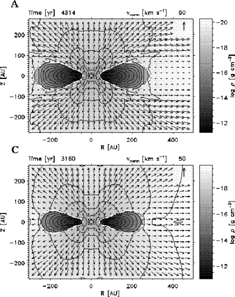
Figure 2: Density, velocity and ionization structure of model A and C. Gray scale and black contour lines display the density structure. These contour lines vary from $\log\rho=-13.0$ to $\log\rho=-19.5$ in increments of $\Delta\log\rho=0.5$. The white contour lines mark the position of the ionization front and the arrows show the velocity field. The normalization is given at the upper right corner.

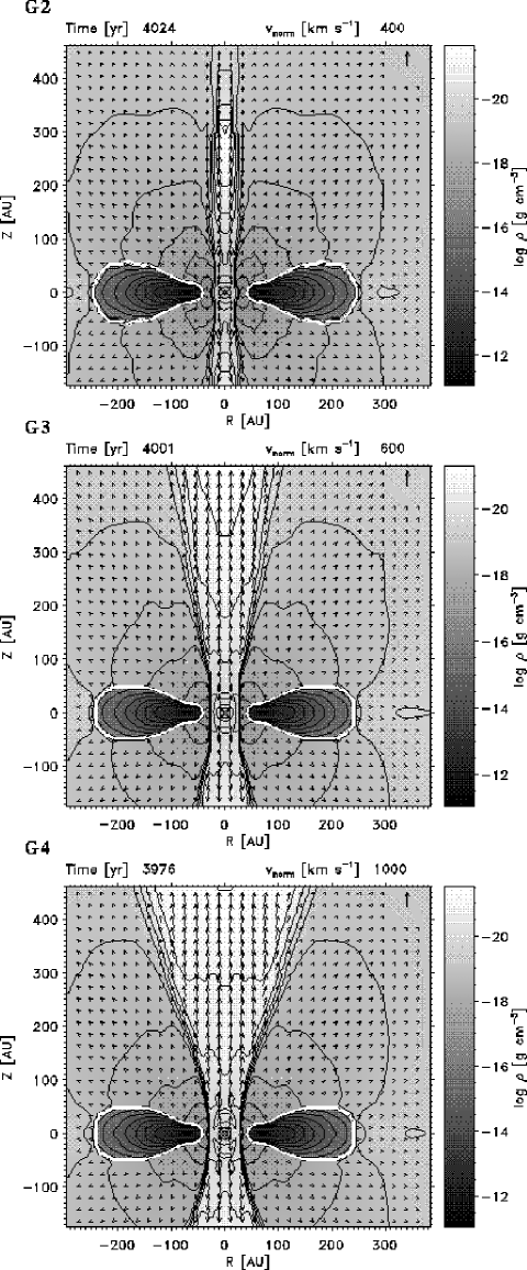
Figure 3: Density, velocity and ionization structure of model G2, G3 and G4. Symbols and lines have the same meaning as in Fig. 2 except the black density contour lines, which are drawn down to $\log\rho=-21.5$.

The underlying numerical models were calculated on five multiply nested grids, each with 62 x 62 grid cells (see Yorke & Kaisig yokai (1995), Paper I, and Paper II). The spatial resolution of the finest grid was $\Delta R=\Delta Z\approx 2\times 10^{13}$ cm (R is the distance to the symmetry axis, Z to the equatorial plane). Axial symmetry and mirror symmetry with respect to the equatorial plane were assumed for the models. The simulations were performed within a volume $(R_{\rm max}^{2}+Z_{\rm max}^{2})^{1/2}\leq 10^{16}$ cm until a quasi-steady state was reached.

For the diagnostic radiation transfer calculations discussed here we use the final states of five simulations described in Paper II. Some of the relevant parameters of these simulations are given in Table 2. Figure 2 and Fig. 3 display the density and ionization structure as well as the velocity field of the selected models. Models A and C are the results of simulations with the same moderate stellar wind and the same radiation source. But in the simulation leading to model A the diffuse uv radiation field originating from scattering on dust grains was completely neglected. For that reason we got a higher photoevaporation rate $\dot{M}_{\rm ph}$ for model C. In Fig. 2 this is recognizable by the greater overall density in the ionized regions and by the higher velocity in the “shadow” regions of the disk in the case of model C. In order to investigate the variation of spectral characteristics with the stellar wind velocity we chose the models with the greatest wind velocities G2, G3 and G4. Figure 3 shows the increasing opening angle of the cone of freely expanding wind with increasing wind velocity.

3.2 Strategy of solution

We use the model data to calculate the ionization structure and the level population. From the level populations we determine the emissivities of each line transition and the continuum emission at each point within the volume of the hydrodynamic model. For each viewing angle $\Theta$ considered, we solve the time independent equation of radiation transfer in a non-relativistic moving medium along a grid of lines of sight (LOS) through the domain, neglecting the effects of scattering:

$$\frac{{\rm d}I_{\nu}}{{\rm d}\tau_{\nu}}=-I_{\nu}+S_{\nu},$$ (16)

where the optical depth is defined as $\tau_{\nu}=\int\kappa_{\nu}{\rm d}s$. Integrations were performed for a given set of frequencies, whereby the effects of Doppler shifts for the line emissivities were taken into account. The resulting intensities are used to determine SEDs, intensity maps and line profiles. Spectra are obtained from the spatial intensity distributions by integration, taking into account that each LOS has an associated “area”. Depending on $\Theta$ the symmetry of the configurations could be utilized to minimize the computational effort (see Fig. 4). For the pole-on view ($\Theta=0^{\circ}$), for example, only a one dimensional LOS array need be considered. For the edge-on view ($\Theta=90^{\circ}$) lines of sight either through a single quadrant (continuum transfer) or through two quadrants (line transfer) are necessary. The resolution of the central regions is enhanced by overlaying a finer LOS grid in accordance with the multiple nested grid strategy used in the hydrodynamic calculations.

Each point in Fig. 4 corresponds to an LOS trajectory through the model. Mapping such a trajectory onto the (R,Z) model grid yields hyperbolic curves as displayed in Fig. 5. Beginning with a starting intensity ($I_{\nu}(-\infty)$), the solution of Eq. (16) is obtained by subdividing the LOS into finite intervals and analytically integrating over each interval assuming a sub-grid model (see below).

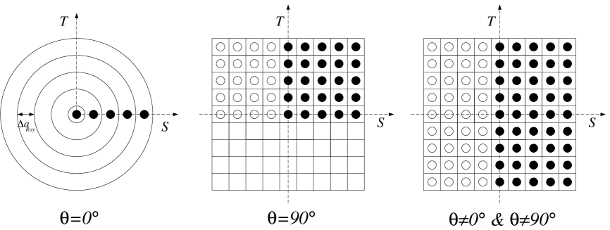
Figure 4: Choice of lines of sight (LOS) and their associated areas for different viewing angles $\Theta$. Filled dots indicate the LOS used for the continuum calculations. Empty dots refer to the additional Lines of Sight necessary for the line profile calculations.

Figure 5: Projection of a typical LOS trajectory (curved dashed line) onto the model data grid (solid lines). Temperature, density, degree of ionization and velocity are defined at cell centers. The small circles divide the LOS into subintervals; the source function $S_{\nu}$ is evaluated at the location of the circles, chosen to lie on the intersections of the LOS with lines connecting the grid cell centers.

3.3 Continuum radiation transfer

If no discontinuities are present within the subinterval under consideration, we assume $S_{\nu}$ varies linearly with $\tau$, i.e.

$$S_{\nu}(\tau)=S_{\nu}^{i}+(S_{\nu}^{i+1}-S_{\nu}^{i})\frac{\tau}{\Delta\tau},$$ (17)

where $i$ and $i+1$ denote the starting and end points of the interval, respectively, and $\Delta\tau$ is a mean optical depth over the interval:

$$\Delta\tau=\frac{\kappa^{i}+\kappa^{i+1}}{2}\Delta s.$$ (18)

With this formulation the solution of Eq. (16) over the entire interval is given by (see Yorke yorke1 (1988)):

$$I_{i+1}=I_{i}\exp(-\Delta\tau) + S_{i}\left[\frac{1-\exp(-\Delta\tau)}{\Delta\tau}-\exp(-\Delta\tau)\right]$$ (19)

$$+ S_{i+1}\left[1-\frac{1-{\rm exp}(-\Delta\tau)}{\Delta\tau}\right].$$

For the cases considered here we choose $I_{0}=0$ as the starting LOS intensity. For “proplyd”-type models (considered in a subsequent paper of this series) a non-negligible background intensity should be specified.

3.4 Radiation transfer in emission lines

For the transitions considered here the radiation field can be considered “diffuse” $I_{\nu}\ll B_{\nu}$ and the contribution of spontaneous emission dominates over line absorption and stimulated emission processes. After separating the source function $S_{\nu}=S_{\rm C}+S_{\rm L}$ and the intensity $I_{\nu}=I_{\rm C}+I_{\rm L}$ of Eq. (16) into the contributions of the continuum and the line, we obtain

$$I_{\rm L}=\frac{\tilde{S}_{\rm L}\exp(-\Delta\tau)}{\sqrt{\pi}\Delta\nu_{\rm th}}\int_{0}^{\Delta\tau}\exp\left[\tau-\left(\frac{\nu-\tilde{\nu}(\tau)}{\Delta\nu_{\rm th}}\right)^{2}\right]{\rm d}\tau,$$ (20)

where ${\rm d}\tau=\kappa_{\rm C}\,{\rm d}s$ and $S_{\rm L}=\epsilon_{\rm L}/\kappa_{\rm C}$. Here $\tilde{\nu}(\tau)$ is the Doppler-shifted frequency of the transition, $\Delta\nu_{\rm th}$ the Doppler width and $\tilde{S}_{\rm L}$ the net source function integrated over the line. Assuming that $\tilde{\nu}$ is linear in $\tau$ over the whole interval yields the analytical solution to Eq. (20):

$$I_{\rm L}=\frac{\tilde{S}_{\rm L}\Delta\tau}{2\Delta\tilde{\nu}}\exp\left(-\frac{(\tilde{\nu}_{2}-\nu)\Delta\tau}{\Delta\tilde{\nu}}\right)\cdot\left[\mbox{erf}(Y_{2})-\mbox{erf}(Y_{1})\right],$$ (21)

where ${\rm erf}(y)=2/\sqrt{\pi}\int_{0}^{z}\exp(-t^{2})dt$ is the error function and $Y_{i}=(\tilde{\nu}_{i}-\nu)/\Delta\nu_{\rm th}$ a dimensionless frequency shift.

The net source function $\tilde{S}_{\rm L}$ is calculated according to the algorithm suggested by Yorke (yorke1 (1988)):

$$\tilde{S}_{\rm L} = \frac{\mbox{erf}(Y_{\rm M})-\mbox{erf}(Y_{\rm 1})}{\mbox{erf}(Y_{2})-\mbox{erf}(Y_{1})}\tilde{S}_{1}+\frac{\mbox{erf}(Y_{2})-\mbox{erf}(Y_{\rm M})}{\mbox{erf}(Y_{2})-\mbox{erf}(Y_{1})}\tilde{S}_{2},$$ (22)

with $Y_{\rm M}=(Y_{1}+Y_{2})/2$. The line source functions $\tilde{S}_{1}$ and $\tilde{S}_{2}$ are calculated from the total line emission coefficient $\tilde{\epsilon}_{\rm L}$ as defined in Eq. (9) at the boundaries of the evaluated interval and from the continuum absorption coefficient: $\tilde{S}_{\rm i}=\tilde{\epsilon}_{\rm L,i}/{\kappa_{\rm C}}$.

If $\Delta\tilde{\nu}\ll\Delta\nu_{\rm th}$, i.e. there is negligible Doppler shift within the subinterval, the solution of Eq. (20) with $\tilde{\nu}_{1}=\tilde{\nu}_{2}=\tilde{\nu}$ is used:

$$I_{\rm L}=\frac{S_{\rm L}}{\sqrt{\pi}\Delta\nu_{\rm th}}\exp\left[-\left(\frac{\nu-\tilde{\nu}}{\Delta\nu_{\rm th}}\right)^{2}\right]\left(1-\exp(-\Delta\tau)\right).$$ (23)

3.5 Treatment of ionization fronts

The numerical models considered contain unresolved ionization fronts due to the coarseness of the hydrodynamic grid. At these positions jumps occur in the physical parameters and the solutions given by Eq. (19) and Eq. (21/23) are poor approximations. The exact location of the fronts within a grid cell are unknown; we assume they lie at the center of the corresponding interval. Our criterion for the presence of an ionization front is a change in the degree of ionization $\Delta x>0.1$ between two evaluation points.

For the continuum calculations Eq. (19) is applied to each half interval with $\Delta\tau=\kappa_{i}\Delta x/2$. For the first half $S=S_{i}$ kept constant and for the second half $S=S_{i+1}$ is held constant. For the line calculations Eq. (23) is used with $\tilde{\nu}=\nu_{1}$ ($\nu_{2}$) and $S_{\rm L}=S_{1}$ ($S_{2}$) for the first (second) half interval.

3.6 Treatment of the central radiation source

The central source is modeled by a black body radiator of temperature $T_{*}$ and radius $R_{*}$. The integration along the line of sight through the center is started at the position of the source with the initial intensity

$$I_{0}=B_{\nu}(T_{*})\frac{R_{*}^{2}\pi}{A},$$ (24)

with $A$ is the area associated with the central LOS.

4 Results

With the code described above we determined SEDs, continuum isophotal maps and line profiles for the forbidden lines [Nii] 6584, [Oii] 3726 and [Oiii] 5007 as well as the H$\alpha$-line for the models introduced in Sect. 3.1. Their relevant physical parameters are listed in Table 2.

4.1 Continuum emission

4.1.1 Spectral Energy Distributions

Figure 6 shows the SEDs of model G2 presented in Paper II for different viewing angles $\Theta$. The spectra can be divided into three regimes dominated by different physical processes:

1. In the frequency range from $10^{8}$ to $10^{11}$ Hz the SED is dominated by the thermal free-free radiation in the ionized region around the dust torus.

2. The ir-excess from $10^{11}$ to $10^{14}$ Hz is due to the optically thick dusty torus itself, which has a mean surface temperature of about 250 K.

3. Beyond $10^{14}$ Hz the SED depends strongly on the viewing angle: if the star is obscured by the dusty torus then the free-free radiation of the Hii-region again dominates the spectrum, otherwise the stellar atmosphere shows up. Due to the uncertainties in the stellar spectra and the neglect of scattering by dust in Eq. (16), which becomes more and more important with increasing frequency, a discussion of the SED beyond $10^{14}$ Hz and comparison with observations are not useful.

Table 2: Scattering coefficient $\kappa^{\rm scat}_{\rm dust}\rho^{-1}$ as well as parameters for the stellar wind (mass loss rate $\dot{M}_{\rm wind}$ and velocity $v_{\rm wind}$) and the ionizing source (stellar photon rate $S_{\rm star}$ and temperature $T_{\rm eff}$) used in the calculations. The evaporation time scale $t_{\rm evap}$ is calculated from $t_{\rm evap}=M_{\rm disk}/\dot{M}_{\rm ph}$ with $M_{\rm disk}=1.67\,M_{\odot}$.

model	$\kappa^{\rm scat}_{\rm dust}/\rho$	$\dot{M}_{\rm wind}$	$v_{\rm wind}$	$\log_{10}S_{\rm star}$	$T_{\rm eff}$	$\dot{M}_{\rm ph}$	$t_{\rm evap}$
	$\mbox{cm}^{2}\mbox{g}^{-1}$	$10^{-8}M_{\odot}\mbox{yr}^{-1}$	$\mbox{km\,s}^{-1}$	$\mbox{s}^{-1}$	K	$10^{-6}M_{\odot}\mbox{yr}^{-1}$	$10^{6}\mbox{yr}$
A	0	2	50	46.89	30 000	0.565	2.96
C	200	2	50	46.89	30 000	1.35	1.24
G2	200	2	400	46.89	30 000	1.65	1.01
G3	200	2	600	46.89	30 000	1.67	1.00
G4	200	2	1000	46.89	30 000	1.64	1.02

According to the analysis of Panagia & Felli (panagia (1975)), who calculated analytically the free-free emission of an isothermal, spherical, ionized wind, the flux density should obey a $\nu^{0.6}$-law:

$$F_{\nu}=6.46\cdot 10^{-3}\;\mbox{Jy}\cdot\left[\frac{\dot{M}}{10^{-5}\mbox{\leavevmode\nobreak\ M}_{\odot}/\mbox{yr}}\right]^{4/3}\cdot\left[\frac{\nu}{10\mbox{\leavevmode\nobreak\ GHz}}\right]^{0.6}\cdot$$

$$\cdot\left[\frac{T}{10^{4}\mbox{\leavevmode\nobreak\ K}}\right]^{0.1}\cdot\left[\frac{d}{\mbox{kpc}}\right]^{-2}\cdot\left[\frac{v_{\rm wind}}{10^{3}\mbox{\leavevmode\nobreak\ km\,s${}^{-1}$}}\right]^{-4/3}.$$ (25)

Schmid-Burgk (schmid (1982)) showed that this holds, modified by a geometry dependent factor of order unity, even for non-symmetrical point-source winds as long as $\rho$ drops as $R^{-2}$. Additionally he postulated that the flux density should hardly be dependent on the angle at which the object is viewed. In Fig. 6 we include for comparison the flux distribution given by Eq. 25 for the photoevaporation rate $\dot{M}_{\rm ph}=1.65\cdot 10^{-6}\;\mbox{M}_{\odot}\mbox{yr}^{-1}$ (see Paper II), $T=10\,000$ K and $v_{\rm wind}=20\;\mbox{km\leavevmode\nobreak\ s}^{-1}$ derived from the line profiles in Sect. 4.2. The slope of the SED in regime 1 is slightly steeper in our results, because our volume of integration is finite; Panagia & Felli (panagia (1975)) derived their analytical results by assuming an infinite integration volume. The flux is almost independent of $\Theta$, which is in good agreement with Schmid-Burgk (schmid (1982)). The deviations between $10^{10}$ and $10^{11}$ Hz are due to the break in the $R^{-2}$-law caused by the neutral dust torus.

Figure 6 also includes the SED of a blackbody at $T=240$ K. The flux $F_{\nu}\propto\nu^{2.2}$ in the far ir between $5\cdot 10^{11}$ Hz and $3\cdot 10^{12}$ Hz is slightly steeper than the comparison blackbody spectrum, because the dust torus is not quite optically thick. With increasing $\Theta$ the maximum shifts towards lower frequencies, because the warm dust on the inside of the torus is being concealed by the torus itself.

We obtain qualitatively the same results for a number of models presented in Paper II.

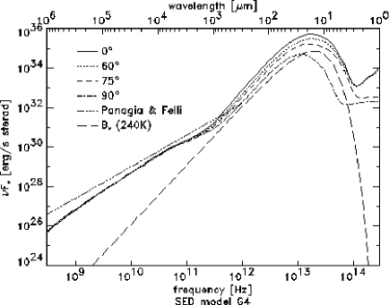
Figure 6: Spectral Energy Distribution for model G2 and different $\Theta$.

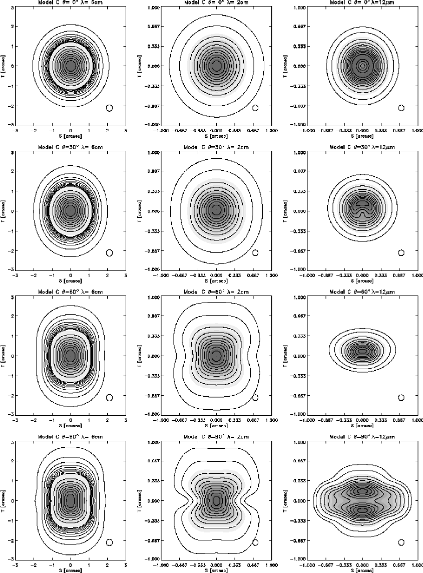
Figure 7: Isophotal maps of model C for different viewing angles and wavelengths as indicated. Assumed distance 300 pc. The circle in the lower right corner marks the FWHM of the point spread function. Values for contours see text.

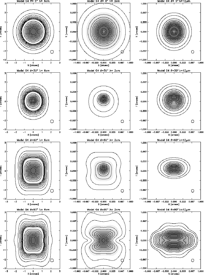
Figure 8: Isophotal maps of model G4 for different viewing angles and wavelengths as indicated. Assumed distance 300 pc. The circle in the lower right corner marks the FWHM of the point spread function. Values for contours see text.

4.1.2 Isophotal maps

We also calculated isophotal maps over the projected $(S,T)$ grid of the sky for models C and G4 (Figs. 7,8). The maps were convolved with a Gaussian point spread function (FWHM 0$.\!\!^{\rm{}^{\prime\prime}}$3 for $\lambda=6$ cm, 0$.\!\!^{\rm{}^{\prime\prime}}$1 for $\lambda=2$ cm and $12\,\mu$m) in order to compare the numerical models with observations of limited resolution. The values (in percent) of the contour lines relative to the maximum flux per beam are 1, 2, 3, 4, 5, 6, 7, 8, 9, 10, 20, 30, 40, 50, 60, 70, 80, 90 for $\lambda=6\,$cm, and 2, 5, 15, 25, 35, 45, 55, 65, 75, 85, 95 for $\lambda=2\,$cm and $12\mu$m.

The difference in these two models is revealed most strikingly in the maps for $\lambda=6\,$cm and $2\,$cm. The mass outflow of model C is more evenly distributed over its whole opening angle, whereas in model G4 most of the mass is transported outward in a cone between $\Theta=30^{\circ}$ and $70^{\circ}$. This leads to the X-shape of the corresponding radio maps for viewing angles $\Theta\geq 60^{\circ}$. The high density in the region between star and disk for this model results in an optically thick torus in this region at $\lambda=2\,$cm. Thus the contours for $\Theta=30^{\circ}$ and $60^{\circ}$ are not symmetric to the equatorial plane at $T=0^{{}^{\prime\prime}}$.

In the maps corresponding to $\Theta=30^{\circ},\lambda=12\mu$m there appears a peculiar horseshoe-like feature. It is generated by the hottest region of the dust torus, which is the innermost boundary with the smallest distance to the star. It can be seen as a ring in the maps for $\Theta=0^{\circ}$. For $\Theta=30^{\circ}$ the part of the ring next to the observer is obscured by the dust torus, whereas the other parts are still visible. The beam width chosen by us allows the resolution of the ring and thus leads to the horseshoe-like feature. For $\Theta=60^{\circ}$ only the most distant part of this hot ring is visible, leading to a maximum in the flux with a smaller spatial extent than for $\Theta=30^{\circ}$.

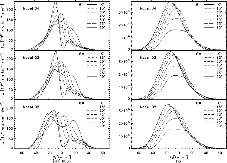
Figure 9: Lines [Nii] 6584 and H$\alpha$ for models G2, G3 and G4, and different “viewing angles” $\Theta$. The models differ only in wind velocity $v_{\rm wind}$.

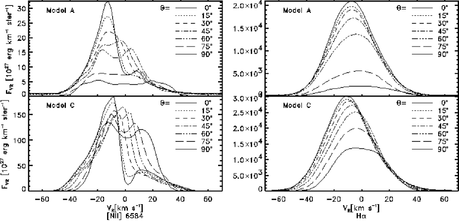
Figure 10: Lines [Nii] 6584 and H$\alpha$ for models A and C, and different “viewing angles” $\Theta$. In model A scattering of uv photons by dust was neglected, in model C included. Note the different scales on the abscissae.

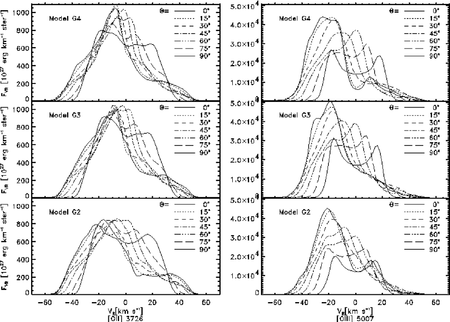
Figure 11: Lines [Oii] 3726 and [Oiii] 5007 for models G2, G3 and G4, and different “viewing angles” $\Theta$. The models differ only in wind velocity $v_{\rm wind}$.

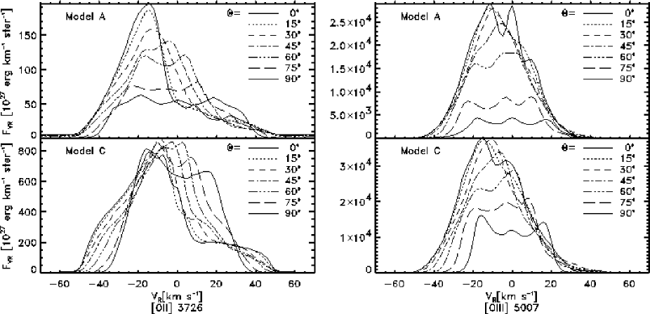
Figure 12: Lines [Oii] 3726 and [Oiii] 5007 for models A and C, and different “viewing angles” $\Theta$. In model A scattering of uv photons by dust was neglected, in model C included. Note the different scales on the abscissae.

4.2 Line profiles

Line profiles can provide useful information on the velocity structure in Hii regions. Because the thermal doppler broadening decreases with increasing atomic weight as $A^{-1/2}$, ions such as Nii and Oiii are better suited for velocity diagnostics than H_α. This can be seen in the line profiles we obtained (Figs. 9-12). They show the flux integrated over the whole area of the object including the disk, the evaporated flow and the cone of the stellar wind. In all cases the line broadening of several ten km s^-1 is dominated by the velocity distribution of the escaping gas. For comparison, the rotational velocity of the dust torus $v_{\rm rot}\simeq 13$ km s^-1 for the inner parts, and the thermal Doppler broadening from Eq. (8) at $T=10\,000$ K is $v_{\rm th}\simeq 9$ km s^-1 for H$\alpha$ and $\simeq 2$ km s^-1 for Oiii.

Figures 10 and 12 show the line profiles for the models A (no scattering of H-ionizing photons) and C (calculated assuming non-negligible uv scattering during the hydrodynamical evolution) from Paper II. uv scattering leads to stronger illumination of the neutral torus by ionizing radiation and thus to a higher photoevaporation rate in model C (by a factor of $\sim 2.3$) compared to model A. Due to the higher density in the regions filled with photoevaporated gas, the lines for model C are generally more intense. In the case of the line [Oii] 3726 one notices that the difference between the fluxes for different angles is the smallest of all transitions. Not only is the density of the outflowing ionized gas higher for case C, but the charge exchange reactions discussed in Sect. 2.2.1 lead to the establishment of a non-negligible Oii-abundance even in the “shadow” regions not accessible to direct stellar illumination. These regions dominate the line spectra for all angles.

Figures 9 and 11 show the calculated line profiles for the models G2, G3 and G4, which only differ by the assumed stellar wind velocity $v_{\rm wind}$, increasing from 400 km s^-1 (G2) to 1 000 km s^-1 (G4). Comparing the results we find two features:

1. The intensity and overall structure of the line profiles considered are almost independent of the stellar wind velocity $v_{\rm wind}$.

2. No high-velocity component appears in the lines due to the stellar wind.

Both features can be explained by the fact that the density of material contained in the stellar wind is much lower than the density in the photoionized outflow. Remembering that $\rho=\dot{M}/4\pi r^{2}v$ in a steady-state outflow and that the line emissivity $\epsilon_{\rm L}\propto\rho^{2}$, we can understand why the low expansion velocities of about $20$ km s^-1 (i.e. material close to the torus) dominate the spectra. The overall evaporation rates as well as the expansion velocities are almost equal for all three models, leading to very similar line profiles. It would be necessary to consider transitions which predominate in hot winds in order to detect this high velocity component and to find significant differences between these models.

In spite of our assumption of optically thin line transfer, the profiles for $\Theta=90^{\circ}$ are not symmetric. This is due to the dust extinction within the Hii-region. The receding material is on average further away from the observer than the approaching. The longer light paths result in stronger extinction of the redshifted components.

We are aware of the fact that the neglection of scattering by dust in Eq. (16) may lead to serious errors in the calculated line profiles. We expect non-negligible contributions especially in the red-shifted parts of the lines due to light scattered by the dense, dusty surface of the neutral torus. This light was originally emitted by gas receding from the torus. The resulting redshift “seen” by the torus remains unchanged during the scattering process and will thus lead to enhancement of the red-shifted wings of the lines.

Nevertheless, we expect our qualitative results still to hold since the arguments mentioned above referring to the geometry of the underlying models are still applicable.

5 Comparison with observations

Although the cases presented here describe the situation of an intermediate mass ionizing source (8.4 M_⊙) with a circumstellar disk, many of the basic spectral features can be generalized. Thus, it is interesting to compare and contrast our results with observed UCHiis, even though many of the central sources are presumably much more massive.

The collections of photometry data in the catalogues of Wood & Churchwell (wood (1989)) and Kurtz et al. (kurtz (1994)) show that the SEDs of almost all UCHii-regions possess roughly the same structure as the ones of the models discussed here: a flat spectrum in the radio and mm regime following a $\nu^{0.6}$-law due to free-free emission and an ir excess originating from heated dust exceeding the free-free emission by $\sim 3-4$ orders of magnitude. A closer inspection shows that the dust temperatures are by an order of magnitude lower in most of the observed sources when compared to our models. This may be an indication that the disks are being photoionized by a close companion in a multiple system rather than the central source. Alternatively, the emitting dust could be distributed in a shell swept up by the expanding Hii-region and thus further away from the exciting star than for the cases discussed here. The large beam width of IRAS and the tendency of massive stars to form in clusters also make it likely that the ir fluxes belong to dust emission caused by more than one heating star. Objects of this type would appear as “unresolved” in the maps presented by Wood & Churchwell (wood (1989)) for distances larger than $\sim$ 300 pc. Due to the cooler dust, the “unresolved” objects cannot be explained by the models of circumstellar disks around uv luminous sources specifically discussed in this paper. Certainly the cometary shaped UCHiis can be explained by a disk being evaporated by the ionizing radiation of an external star and interaction with its stellar wind. Numerical models dealing with this scenario will be presented in the next paper of this series.

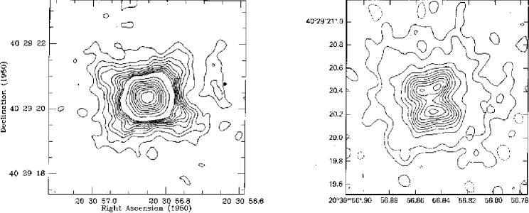
Figure 13: VLA-maps of MWC~349. Left: $\lambda=$ 6 cm (Cohen et al. cohen (1985)), FWHM $=$ 0$.\!\!^{\rm{}^{\prime\prime}}$3. Contour levels at 1, 2,…, 9, 10, 20,…, 80, 90% of maximum flux 16,59 mJy beam^-1. Right: $\lambda=$ 2 cm (White & Becker white (1985)), FWHM $=$ 0$.\!\!^{\rm{}^{\prime\prime}}$1. Contour levels at $-2$, 2, 5, 15, 25,…95% of maximum flux 156 mJy beam^-1.

5.1 MWC~349 A

A commonly accepted candidate for an evaporating disk around a young massive star is MWC~349 A. Its radio continuum flux obeys the $\nu^{0.6}$-law up to $\lambda=30$ cm (see collection of photometry results in Thum & Martín-Pintado thum (1993)). Radio maps obtained by Cohen et al. (cohen (1985)) and White & Becker (white (1985)) show an extended ionized bipolar outflow with a peculiar X-shape (Fig. 13). In the center Leinert (leinert (1986)) finds an elongated, dense clump with $T\sim 900\,$K, with optically thick ir emission, which makes MWC~349 A one of the brightest IRAS sources. The elongated structure shows an almost Keplerian velocity profile along its major axis, perpendicular to the outflow axis (Thum & Martín-Pintado thum (1993)). This leads to the assumption of a neutral dust torus around the central star with a small outer radius $<100\,$AU. Kelly et al. (kelly (1994)) estimated the extinction towards this early-type star to be $A_{\rm V}=10.8$.

The SED of MWC~349 A shows all the features which we find for our models. The extinction and the geometry of the outflow, as well as the lack of a high-velocity component in the line profiles (Hartmann et al. hartmann (1980), Hamann & Simon hamann (1988)), could be explained by a model with fast stellar wind presented in this paper, assuming a viewing angle $\Theta\sim 90^{\circ}$. On the other hand, the high dust temperatures in the torus, $T_{\rm d}\sim 800$ K, and the extremely high mass loss rate in the outflow, $\dot{M}=(1.16\pm 0.05)\times 10^{-5}\,$M_⊙ yr^-1 (Cohen et al. cohen (1985)) remain puzzling and need clarification by a numerical model after the method described in this series but especially “tailored” to suit the needs of MWC~349 A.

6 Conclusions

In this paper we showed that the models of photoevaporating disks around intermediate mass stars cannot explain the large number of “unresolved” UCHii’s observed by Wood & Churchwell (wood (1989)) and Kurtz et al. (kurtz (1994)), because the inferred dust temperatures of these objects are in most cases an order of magnitude lower than those obtained in the numerical models. But the question remains whether the disks of more massive stars than considered here could be responsible for the high abundance of the “unresolved” UCHii’s. Disks around close companions of massive stars should be treated in greater detail. If we assume that circumstellar disks are the rule in the process of star formation, the simplicity and straightforwardness of the model make it favorable compared to alternative suggestions. The extremely high radiation pressure in the vicinity of massive stars could lead to a larger distance between star and disk and thus to smaller dust temperatures.

Another important result of this work is that the profiles of forbidden lines in the optical for the models G2, G3 and G4 with wind velocities of $400-1000$ km s^-1 are almost independent of $v_{\rm wind}$. This is due to the fact that the mass loss rate and velocity of the evaporated disk material is not affected by its interaction with the stellar wind, but by the rate of ionizing photons and the peculiar shock structure which is very similar in the numerical models (see Fig. 3). Since the total mass loss rate is dominated by the evaporated component with low velocity, and the emission is proportional to $\rho^{2}$, the intensity in the lines does not depend on details of the stellar wind and their profiles show the same low-velocity components.

Treatment of optically thick line emission and scattering effects is not possible with the method presented above. In order to compare non-LTE-effects like masing lines, which are observed in various objects related with the formation of massive stars, one has to refer to different methods, e.g. the Monte-Carlo method presented by Juvela (juvela (1996)). This would immensely help us in our understanding of the process of formation and evolution of massive stars.

- (1) Aldrovandi S.M.U., Pequinot D., 1973, A&A, 25, 137
- (2) Aldrovandi S.M.U., Pequinot D., 1976, A&A, 47, 321
- (3) Arnaud M., Rothenflug R., 1985, A&AS, 60, 425
- (4) Cohen M., Bieging J.H., Welch W.J., Dreher J.W., 1985, ApJ, 292, 249
- (5) De Pree C.G., Rodríguez L.F., Goss W.M., 1995, Rev. Mex. Astron. Astrofis., 31, 39
- (6) García-Segura G., Franco J., 1996, ApJ, 469, 171
- (7) Hamann F., Simon M., 1988, ApJ, 327, 876
- (8) Hartmann L., Jaffe D., Huchra J.P., 1980, ApJ, 239, 905
- (9) Henry R., 1970, ApJ, 161, 1153
- (10) Hollenbach D.J., Johnstone D., Shu F.H., 1993, ASP Conf. Ser., 35, eds. J.P. Cassinelli and E.B. Churchwell, p. 26.
- (11) Hollenbach D.J., Johnstone D., Lizano S., Shu F.H., 1994, ApJ, 428, 654
- (12) Hummer D., Storey P., 1971, MNRAS, 224, 801
- (13) Juvela M., 1996, A&A, 322, 943
- (14) Kelly D.M., Rieke G.H., Campbell B., 1994, ApJ, 425, 231
- (15) Kurtz S., Churchwell E., Wood D.O.S., 1994, ApJS, 91, 659
- (16) Leinert C., 1986, A&A, 155, L6
- (17) Nussbaumer H., Storey P., 1983, A&A, 126, 75
- (18) Osterbrock D., 1961, ApJ, 135, 195
- (19) Osterbrock D., 1989, Astrophysics of Gaseous Nebula and Active Galactic Nuclei, University Science Books, 20 Edgehill Road, Mill Valley, CA 94941
- (20) Panagia N., Felli M., 1975, A&A, 39, 1
- (21) Preibisch Th., Ossenkopf V., Yorke H.W., Henning Th., 1993, A&A, 279, 577
- (22) Reid M.J., Haschick A.D., Burke B.F., Moran J.M., Johnston K.J., Swenson G.W. 1981, ApJ, 239, 89
- (23) Richling S., Yorke H.W., 1997, A&A, 327, 317 (Paper II)
- (24) Schmid-Burgk J., 1982, A&A, 108, 169
- (25) Shull J.M., Van Steenberg M., 1982, ApJS, 48, 95
- (26) Spitzer, Jr. L., 1969, Diffuse Matter in Space, Interscience Tracts on Physics and Astronomy, Vol. 28, Interscience Publishers Inc.
- (27) Thum C., Martín-Pintado J., 1993, ASP conference series, Vol. 62, eds. P.S. The, M.R. Perez, P.J. v.d. Heuvel
- (28) Watson A.M., Hanson,M.M., 1997, ApJL, 490, 165, astro-ph/9709120
- (29) White R.L., Becker R.H., 1985, ApJ, 297, 677
- (30) Wood D.J.S., Churchwell E., 1989, ApJS, 69, 831
- (31) Xie T., Mundy L.G., Vogel S.N., Hofner P., 1996, ApJL, 473, 131, astro-ph/9610054
- (32) Yorke H.W., 1988, Radiation in Diffuse Matter, in: Kudritzki, R.P., Yorke, H.W., Frisch, H. 1988, Radiation in Moving Gaseous Media, 18th Saas Fee Course, Geneva Observatory
- (33) Yorke, H.W. 1995, in: Circumstellar Disks, Outflows, and Star Formation, eds. S. Lizano, J.M. Torrelles, RevMexAASC, 1, 35
- (34) Yorke, H.W., Kaisig, M. 1995, Comp. Phys. Comm., 89, 29
- (35) Yorke H.W., Welz A., 1993, in: Star Formation, Galaxies and the Interstellar Medium, eds. J. Franco, F. Ferrini, G. Tenorio-Tagle, (Cambridge: Cambridge Univ. Press), p. 239.
- (36) Yorke H.W., Welz A., 1996, A&A, 315, 555 (Paper I)