Electron acceleration in SNR and diffuse gamma-rays above 1 GeV

Abstract

The recently observed X-ray synchrotron emission from four supernova remnants (SNR) has strengthened the evidence that cosmic ray electrons are accelerated in SNR. We show, that if this is indeed the case, the local electron spectrum will be strongly time-dependent, at least above roughly 30 GeV. The time dependence stems from the Poisson fluctuations in the number of SNR within a certain volume and within a certain time interval. As far as cosmic ray electrons are concerned, the Galaxy looks like actively bubbling swiss cheese rather than a steady, homogeneously filled system.

Our finding has important consequences for studies of the Galactic diffuse gamma-ray emission, for which a strong excess over model predictions above 1 GeV has been reported recently. While these models were relying on an electron injection spectrum with index 2.4 – chosen to fit the local electron flux up to 1 TeV – we show that an electron injection index of around 2.0 would a) be consistent with the expected Poisson fluctuations in the locally observable electron spectrum and b) explain the above mentioned gamma-ray excess above 1 GeV. An electron injection index around 2 would also correspond to the average radio synchrotron spectrum of individual SNR. We use a three-dimensional propagation code to calculate the spectra of electrons throughout the Galaxy and show that the longitude and latitude distribution of the leptonic gamma-ray production above 1 GeV is in accord with the respective distributions for the gamma-ray excess.

We finally point out that our model implies a strong systematic uncertainty in the determination of the spectrum of the extragalactic gamma-ray background.

1 Introduction

As was first observed by OSO-3 (Kraushaar et al. (1972)), the dominant feature of the high-energy $\gamma$-ray sky is the intense emission from the Galactic plane. Later the complete SAS-2 (Fichtel et al. (1975)) and COS-B (Mayer-Hasselwander et al. (1982)) data gave evidence for a correlation between the $\gamma$-ray emission and the spatial structures of the Galaxy. The intensity distribution and the spectral form of the emission have led to the consensus that the diffuse $\gamma$-ray radiation is primarily produced by interactions between Galactic cosmic ray particles and the interstellar medium, and to a small extent by unresolved Galactic point sources (Bloemen (1989); Strong (1995)). The EGRET observations of the Magellanic Clouds have shown that cosmic ray nucleons in the energy range below 100 GeV are almost certainly galactic (Sreekumar et al. (1993)), while the observations made with the OSSE and COMPTEL instruments aboard CGRO have provided strong evidence that cosmic ray electrons are galactic (Schlickeiser et al. (1997), see also Fazio et al. (1966)). Therefore the diffuse Galactic $\gamma$-ray emission tells us about the propagation of cosmic rays from their sources to the interaction regions and thus complements the direct particle measurements by balloon and satellite experiments.

The greater sensitivity and spatial and energy resolution of EGRET compared with SAS-2 and COS-B permit a much more detailed analysis of the diffuse Galactic $\gamma$-ray emission than was possible with the earlier experiments. The spatial and spectral distribution of the diffuse emission within $10^{\circ}$ of the Galactic plane have recently been compared with a model calculation of this emission which is based on realistic interstellar matter and photon distributions and dynamical balance (Hunter et al. (1997)), i.e. cosmic rays having the same spectrum and composition everywhere in the Galaxy and having an intensity which follows the surface density of thermal gas convolved with a Gaussian with dispersion $\sigma=1.7\,{\rm kpc}\ -\ 2.0\,{\rm kpc}$ (Bertsch et al. (1993)). The distribution of the total intensity above 100 MeV agrees surprisingly well with the model predictions. However, at higher energies above 1 GeV the model systematically underpredicts the $\gamma$-ray intensity. If the model is scaled up by a factor 1.6, the model prediction and the observed intensity above 1 GeV agree well. Thus the model displays a deficit of $\sim$38% of the total observed emission which depends, if at all, only weakly on location. At energies above 1 GeV around 90% of the model intensity is due to $\pi^{0}$-decay, i.e. hadronic processes, and only 10% is due to interactions of electrons.

There are a number of possible explanations for this deficit:

– A miscalibration of EGRET could cause an overestimation of the intensity above 1 GeV. This possibility is highly unlikely. Point sources generally show power-law spectra without spectral hardening above 1 GeV. It would require an extreme level of cosmic conspiracy for a calibration error to mimic a general power-law behavior in the spectra of cosmic $\gamma$-ray sources.

– The kinematics of $\pi^{0}$ production may be poorly understood. Detailed Monte-Carlo calculations have shown (Mori (1997)), that models based on the current knowledge of particle interactions do not give very different results for the $\pi^{0}$ spectra than do simple isobar plus scaling descriptions (Dermer (1986)). It is unlikely that the cosmic ray nucleon spectrum in the solar vicinity is softer than that elsewhere in the Galaxy. The local cosmic ray spectrum samples sources within a few kpc in distance and a few times 10⁷ years in time. Since the observed deficit appears to be independent of Galactic longitude, the sources of cosmic rays within a few kpc from the sun would have to be different from those in the inner Galaxy and those in the outer Galaxy. We have also tested and verified that the uncertainties in the local interstellar cosmic ray spectrum below a few GeV are by far not sufficient to account for the deficit. The uncertainties arising from our limited knowledge of the cosmic ray nucleon spectrum and the nucleon-nucleon interaction kinematics can be estimated to be on the order of a few percent.

– There may be unresolved point sources which contribute strongly at higher $\gamma$-ray energies. The only known class of objects with appropriate spectra is pulsars. Based on the properties of the six identified $\gamma$-ray pulsars it has been found that unresolved pulsars would indeed contribute mainly between 1 GeV and 10 GeV (Pohl et al. 1997a ). However, to account for all the deficit it is required that more than 30 pulsars be detectable by EGRET as point sources. This can be compared with less than 10 unidentified $\gamma$-ray sources which are not variable (McLaughlin et al. (1996)) and which show pulsar-like spectra (Merck et al. (1996)). Also, the latitude distribution of the $\gamma$-ray emission from unresolved pulsars is inconsistent with that of the observed emission. Unresolved pulsars will contribute 6-10% of the observed $\gamma$-ray intensity above 1 GeV and around 3% in the energy band between 100 MeV and 1 GeV (Pohl et al. 1997a ), and thus they can account only for a small fraction of the high-energy $\gamma$-ray deficit.

All in all the effects described above can account only for a small fraction of the deficit, or can add only small systematic uncertainties. In this paper we will investigate whether the remaining deficit of 30-35% may be caused by inverse Compton emission of high-energy electrons. Leptonic processes contribute only around 10% of the intensity above 1 GeV in the model of Hunter et al. (1997), which corresponds to $\sim$6% of the total observed intensity. Thus the leptonic contribution would have to be increased to 35-40% of the total observed emission to explain all the deficit.

The Galactic distribution of cosmic ray electrons is intimately linked to that of their sources. The recently-found evidence of X-ray synchrotron radiation from the four supernova remnants SN1006 (Koyama et al. (1995)), RX J1713.7-3946 (Koyama et al. (1997)), IC443 (Keohane et al. (1997)), and Cas A (Allen et al. (1997)) supports the hypothesis that Galactic cosmic ray electrons are accelerated predominantly in SNR. X-ray synchrotron radiation implies TeV $\gamma$-ray emission from the comptonization of the microwave background at a flux level which depends only on the average magnetic field strength (Pohl (1996)), and indeed the detection of the remnant SN1006 at TeV energies has been announced recently (Tanimori et al. (1997)). Interestingly, there is no clear observational proof that the nuclear component of cosmic rays is accelerated likewise in SNR. The acceleration of cosmic ray nucleons in SNR should lead to observable flux levels at TeV energies (Drury, Aharonian and Völk (1994)), however with a spectrum different from that of the leptonic emission. The generally tight upper limits for TeV emission from the nearest SNR (Lessard et al. (1995); Buckley et al. (1998)) are in conflict with simple shock acceleration models for cosmic ray nucleons in SNR.

Most of the radio synchrotron spectra of SNR can be well represented by power-laws with indices around $\alpha\simeq 0.5$, corresponding to electron injection indices of $s\simeq 2.0$ (Green (1995)). This is in accord with predictions based on models of particle acceleration (Blandford and Eichler (1987)). However, it is different from the electron injection spectral index of $s=2.4$ which has been inferred from the locally observed electron spectrum (Skibo (1993)) and which subsequently has been used in the model of Galactic $\gamma$-ray emission of Hunter et al. (1997). The contribution of cosmic ray electrons to the Galactic $\gamma$-ray spectrum at high energies depends strongly on their injection spectral index. If the acceleration cut-off energy is high enough, the leptonic $\gamma$-ray emission may even dominate at TeV-PeV energies (Porter and Protheroe (1997)). A change in the electron injection index by $\delta s=0.4$ could increase the inverse Compton emissivities at a few GeV by an order of magnitude or more.

Let us suppose that for some reason the local cosmic ray electron spectrum is different from the average electron spectrum in the Galaxy. Then the following scenario appears viable: the bulk of cosmic ray electrons is accelerated in SNR with an injection index around $s\simeq 2.0$. The leptonic $\gamma$-ray emission at a few GeV would be much stronger than in the Hunter et al. model, and it may explain a substantial fraction of the discrepancy between their model and the observed spectra. So if we would find a mechanism or an effect which would cause the local electron spectrum to be different from the Galactic average, we may in a second step reassess the $\gamma$-ray spectra produced by Galactic cosmic rays without having to assume an electron injection index of $s=2.4$.

It has been noted before that the spatial distribution of cosmic ray sources affects the locally observable spectra (Cowsik and Lee (1979); Lerche and Schlickeiser 1982a ). As far as electron acceleration in SNR is concerned, there is no evidence that the star formation activity and thus the SNR production rate in the solar vicinity is significantly less than the Galactic average. In the next section we will show that for cosmic ray electrons, unlike nucleons, the local spectra above a certain energy can deviate from the Galactic average, even if the spatial distribution of cosmic ray accelerating SNR is homogeneous. This is a result of the discrete nature of SNR both in space and in time. We will use this finding in the third section to model the high-energy $\gamma$-ray excess as result of inverse Compton emission of cosmic ray electrons, albeit with a harder injection spectrum than conventionally assumed.

2 The time-dependence of the local electron spectrum

The spectrum of cosmic ray electrons in terms of the contributions of discrete sources like supernova remnants (SNR) has been discussed before (Cowsik and Lee (1979)). These authors have investigated the case of continuously active sources and have concluded that one needs sources situated within a few hundred parsecs of the solar system, in order that the energy losses of electrons do not induce a cutoff in the energy spectrum. Since the required number of active sources exceeds that of supernova remnants by an order of magnitude, SNR were found unlikely to be the only source of cosmic ray electrons between 1 GeV and 1 TeV. In that paper the diffusion coefficient had been assumed independent of energy. With the usual energy dependence $D\propto E^{(0.3-0.6)}$ some of the statements in the Cowsik and Lee paper would have to be relaxed.

In this section we will also consider the finite lifetime of SNR or other possible cosmic ray accelerators together with the random distribution of SNR in space and time. The latter induces a time dependence in the local electron spectrum at higher energies, which stems from the Poisson fluctuations in the number of SNR within a certain distance and within a certain time interval. As we will see, the discreteness of sources does not simply cause a cutoff in the electron spectrum, but makes it time variable and thus unpredictable beyond a certain energy.

Since effects of the discreteness of sources show up only at higher particle energy, we may describe the propagation of cosmic ray electrons at energies of 1 GeV to 1 TeV by a simplified transport equation

$${{\partial N}\over{\partial t}}-{{\partial}\over{\partial E}}(bE^{2}\,N)-D\,E^{a}\,\nabla^{2}N=Q$$ (1)

where we consider continous energy losses by synchrotron radiation and inverse Compton scattering, an energy-dependent diffusion coefficient $D\,E^{a}$, and a source term $Q$. The Green’s function for this problem can be found in the literature (Ginzburg and Syrovatskii (1964)).

$$G(r,r^{\prime},t,t^{\prime},E,E^{\prime})={{\delta\left(t-t^{\prime}+{{E-E^{\prime}}\over{b\,E\,E^{\prime}}}\right)}\over{bE^{2}\,\left(4\pi\,\lambda(E,E^{\prime})\right)^{3/2}}}\ \exp\left(-{{(r-r^{\prime})^{2}}\over{4\,\lambda(E,E^{\prime})}}\right)$$ (2)

where

$$\lambda(E,E^{\prime})={{D}\over{b\,(1-a)}}\ \left(E^{a-1}-E^{\prime a-1}\right)$$ (3)

In case of discrete sources the injection term $Q$ is a sum over all sources. For an individual source showing up at time $t_{0}$ and injecting for a time period $\tau$ we can write

$$Q_{i}=q_{0}\,E^{\prime-s}\,\delta(r^{\prime})\,\Theta(t^{\prime}-t_{0})\,\Theta(t_{0}+\tau-t^{\prime})$$ (4)

Without loss of generality we can set $t=0$ and obtain

$$N=q_{0}\,E^{-s}\int_{-{{1}\over{bE}}}^{0}\ dt^{\prime}\ {{\Theta(t^{\prime}-t_{0})\,\Theta(t_{0}+\tau-t^{\prime})\,\exp\left(-{{r^{2}}\over{4\Lambda}}\right)}\over{\left(4\pi\Lambda\right)^{3/2}\ (1+bEt^{\prime})^{2-s}}}$$ (5)

where

$$\Lambda={{D\,E^{a-1}}\over{b\,(1-a)}}\ \left(1-(1+bEt^{\prime})^{1-a}\right)$$ (6)

and $r$ is the distance between source and observer. $N$ is the contribution to the local electron spectrum provided by a single source (SNR) at distance $r$ which is (was) injecting electrons for a time period $\tau$ starting at $t_{0}$. The local spectrum of electrons can now be obtained by summing the contributions from all individual sources. In our case the distribution of SNR is, for ease of exposition and computation, assumed to be a homogeneous disk of radius $r_{s}=15\,$kpc and half-thickness $z_{s}=0.14\,$kpc. Other choices for the spatial distribution of SNR do not impose serious changes in the results, as long as the distribution is not structured on sub-kpc scales.

The numerical procedure is as follows: for each volume element $\delta V$ the expected number of SNR injecting cosmic rays within the time interval $\delta t$ is

$$N_{\lambda}={{\delta V\ \delta t}\over{V_{tot}\ t_{inj}}}$$ (7)

where $V_{tot}$ is the total volume of the source distribution and $t_{inj}=55\,$years is the inverse of the supernova rate (Cappelaro et al. (1997)). $\delta t$ has to be the maximum lookback time in our model which is the sum of the SNR lifetime $\tau$ and the electron energy loss time $t_{l}={{1}\over{b\,(1\,{\rm GeV})}}$ at 1 GeV, the lowest energy considered here. At a given time the actual number of SNR in that volume element is a Poissonian random number with mean $N_{\lambda}$, and each of the SNR has a birth date which is a random number uniformly distributed within $[-\tau-t_{l},0]$. The final electron spectrum is then derived by summing over the contributions of the individual SNR per volume element and summing over all relevant volume elements. We calculate 400 such ‘random’ spectra and thus derive the distribution of possible spectra and their spread.

In Fig.1 we show the resulting range of local electron spectra compared with the observed spectra (Ferrando et al. (1996); Golden et al. (1994, 1984); Tang (1984); Taira et al. (1993)). The energy density of the ambient photon fields plus that of the perpendicular component of the magnetic field strength is in total taken to be 3.5 eV/cm³. The changes in the Compton cross section in the Klein-Nishima regime of optical and near-infrared photon fields are neglected. The diffusion coefficient is $D=4\cdot 10^{27}\ {\rm cm^{2}\,sec^{-1}}$ at 1 GeV and increases with energy to the power a=0.6, in accord with results for a two-dimensial diffusion model fit to the local spectra of 13 primary and secondary cosmic ray nuclei at rigidities between 1 GV and 10³ GV (Webber, Lee and Gupta (1992)). At these energies electrons and nuclei will scatter off the same turbulence, except for the helicity, and thus their diffusion behaviour may be expected to be similar. The injection spectral index of electrons is s=2.0, which corresponds to the mean synchrotron spectral index of individual SNR (Green (1995)).

The solar modulation of electrons at a few GeV energy has a strong effect on the observed spectrum. Note the difference between the spectrum observed when the modulation level was high (Golden et al. (1994)) and the spectrum observed during the passage of Ulysses over the solar south pole (Ferrando et al. (1996)). We have crudely approximated the effect of solar modulation using the force-field approach (Gleeson and Axford (1968)) with $\Phi=400\,MV$. Thus we probably overestimate the modulation in case of the Ulysses data and underestimate in case of the Golden et al. data.

The spectra at a given time are not necessarily smooth. There is no preference for the usual broken power-laws or power-laws with exponential cut-offs. In fact the individual spectra are bumpy above $\sim$ 50 GeV and some display step-like features. As an example we show a particular spectrum as dash-dotted line in Fig.1, which is slightly on the low side between 10 GeV and 100 GeV, where it suffers further softening before it abruptly hardens at 300 GeV.

Below 10 GeV the local electron spectrum is well determined. Between 10 GeV and 100 GeV it varies with time by a factor of 2 or 3, and above 100 GeV is completely unpredictable. Changes in the absolute numbers for the diffusion coefficient and the radiative energy losses do not change the basic behaviour, but can shift the transition between weak and strong variability to lower or higher energies. If the energy dependence of the diffusion coefficient is weaker, i.e. $a<0.6$, the transition between weak and strong variability will be faster, and vice versa (a slower transition for higher powers than a=0.6). For comparison we have indicated the result for an energy dependence of the diffusion coefficient, $D\propto E^{0.33}$.

As shown in Fig.1, the high-energy data for the local electron flux are in accord with an injection spectral index of s=2.0, though in a model with steady injection and a smooth source distribution these data would require an injection index of around 2.4 (Skibo (1993)). Concerning the distribution of high-energy electrons, the Galaxy would look like swiss cheese, with holes and regions of higher density. In the line-of-sight integrals, which are relevant for comparison with the EGRET $\gamma$-ray data, the averaging over holes and high-density regions will give the same result as a model with steady injection, however with source index of 2.0 instead of 2.4. At higher latitudes the line-of-sight will be so short that regions of low or high electron density will be resolved. The leptonic $\gamma$-ray spectra in direction of the Galactic poles should be relatively soft since the line-of-sight integral of the $\gamma$-ray emissivity will be dominated by the soft local spectrum.

The absolute electron flux is reproduced if each SNR provides an energy input of $10^{48}\,{\rm ergs}$ in the form of electrons, which is one thousandth of the canonical value of $10^{51}\,{\rm ergs}$ for the kinetic energy input per supernova. Taken over a lifetime of $10^{5}\,{\rm years}$ the corresponding power of $5\cdot 10^{35}\,{\rm ergs/sec}$ is less than the X-ray luminosity of SN1006 alone.

The time variability of the high energy cosmic ray spectrum will not be related or even be synchronous to variability in the flux of low-energy cosmic ray nucleons, which can be traced by cosmogenic instable isotopes in sediments (Sonnett et al. (1987); McHargue, Damon and Donahue (1995); Kocharov (1996)) or meteorites (Bonino (1996)).

A few notes should be added. We have taken supernova explosions to be completely independent of each other. One may expect some level of correlation in OB associations and SNOBs, which would make the basic effect of time dependence even more dramatic, since the OB associations and SNOBs would act as single sources with longer lifetime, but much smaller frequency of occurrence.

Another important point is that we have assumed that all electron sources produce the same spectrum. In reality this doesn’t need to be the case. Some SNR will produce electrons with harder spectrum, and another group of SNR will provide softer spectra. It may be that the spectral form depends on the age of an SNR. In fact the radio data show that SNR do have different synchrotron spectra (Green (1995)). If we take the electron injection spectral index of an individual SNR not as a fixed number, but a random variable following some probability function, the time-averaged spectrum (the dotted line in Fig.1) will get a positive curvature. The level of time variability on the other hand will get larger. The shaded regions in Fig.1, in which the spectrum is contained for 68%, respectively 95%, of the time, extend beyond those for fixed injection index.

A final note concerns secondary positrons and electrons. These particles are generated subsequent to interactions of cosmic ray nucleons with ambient gas, and hence the effect discussed does not apply and the local spectrum of secondary electrons will not vary. Thus the observed positron fraction will also exhibit variability anticorrelated with that of the primary electron spectrum. If we are indeed living in a hole in the distribution of high-energy electrons then the positron fraction above, say, 20 GeV will be above the level expected in steady injection models, if the gas density within $\sim\,$1 kpc from the sun is not also sub-average. This may explain the observed positron fraction in that energy range, which is indeed slightly above the model predictions (Barwick et al. (1997)).

We have seen that the discreteness of sources of cosmic ray electrons causes a strong variability of the local electron spectrum at higher energies. Therefore the high energy electron spectrum does not prescribe our choice of electron injection spectrum in propagation models.

If we consider $\gamma$-ray emission in the Galactic plane, the line-of-sight integral of the emissivity will correspond to an averaging over the different variability states, and hence the $\gamma$-ray intensity calculated with time-dependent models will not differ significantly from the results of steady-state models. The latter are much easier to compute and thus preferrable, but they will in general not be able to reproduce the local high energy electron spectrum correctly. On the other hand, in the absence of reliable data on the position and age of all nearby SNR it is also impossible to calculate the time-dependent local electron spectrum precisely, we can only infer the level of variability. Therefore we feel that, if the acceleration of electrons occurs predominantly in SNR, the $\gamma$-ray emission in the Galactic plane can be sufficiently well described with steady-state models, provided the model is not required to fit the local electron data above $\sim\,$30 GeV. In the next section we will discuss a steady-state model for the diffuse leptonic $\gamma$-ray emission for an injection index of 2.0.

3 The propagation of electrons in the steady state case

There is a richness of literature on the topic of electron propagation in the Galaxy, including analytical solutions for the one- or two-dimensional diffusion and diffusion-convection problem (Ginzburg and Syrovatskii (1964); Berkey and Shen (1969); Lerche and Schlickeiser (1981); Lerche and Schlickeiser 1982b ; Pohl and Schlickeiser (1990)). These solutions can be well described in their basic behavior by the concept of the catchment sphere (Webster (1970)). The energy losses prevent electron propagation farther from their source than a critical distance $\rho$ which is defined by equality of the time scales for transport and for energy losses, so that the spatial dependence of the Green’s function of the problem is basically a function which is a constant for distances less than $\rho$ and which is zero beyond $\rho$. If the transport is governed by diffusion and if the energy loss terms do not strongly depend on location, then $\rho$ will not strongly depend on direction, and thus a source of cosmic rays at the position $(x^{\prime},y^{\prime},z^{\prime})$ would fill a sphere of radius $\rho$ with cosmic rays. Hence we may separate the spatial problem and the energy problem, and approximate the solution to the spatial problem by a Gaussian function for the catchment sphere. The Gaussian function is exact at higher energies where radiative energy losses dominate, but is a crude approximation at very low energies, where ionization and Coulomb losses are important.

We will include escape as a catastrophic loss term, which limits $\rho$ to some maximum value. This approximates the effect of a sudden increase of the diffusion coefficient at a certain height above the Galactic plane (Lerche and Schlickeiser 1982b ). We regard this a better description than a finite boundary with density and density gradient set to zero at $L_{halo}$, a few kpc above the Galactic plane, since for a physical escape solution the density outside the diffusion region relates to that inside as

$$n_{out}\simeq{{n_{in}\,L_{halo}}\over{\tau_{esc}\,\beta\,c}}\simeq 10^{-4}\ n_{in}\left({{E}\over{\rm GeV}}\right)^{0.6}$$ (8)

and thus it is definitely not zero. With a diffusion coefficient $D=D_{0}\,E^{a}$, $E$ being the kinetic energy, we have

$$\rho(E)=\sqrt{4\,D_{0}\,E^{a}}\,\sqrt{\tau_{eff}}$$ (9)

where

$$\tau_{eff}^{-1}=\tau_{esc}^{-1}+\tau_{loss}^{-1}$$ (10)

We can write the differential number density of cosmic rays at position $(x,y,z)$ coming from a source at $(x^{\prime},y^{\prime},z^{\prime})$ as

$$\delta N={1\over{(\sqrt{\pi}\,\rho)^{3}\,|{\dot{E}}|}}\$$

$$\qquad\quad\times\int_{E}du\ Q(u)\,{\rm exp}\left(-\smallint_{E}^{u}{{dv}\over{\tau_{esc}(v)\,|\dot{E}(v)|}}\right)\ {\rm exp}\left(-{{r^{2}}\over{\rho^{2}}}\right)$$ (11)

where

$$r^{2}=(x-x^{\prime})^{2}+(y-y^{\prime})^{2}+(z-z^{\prime})^{2}\ ,$$ (12)

$\dot{E}$ is the energy loss term and $Q(E)$ is the source spectrum at position $(x^{\prime},y^{\prime},z^{\prime})$. Physically $\delta N$ is a propagator and it can be treated like a Green’s function. Given the spatial distribution of sources $q(x^{\prime},y^{\prime},z^{\prime})$ we obtain the cosmic ray spectrum at any position $(x,y,z)$ as

$$N(E)=\int dx^{\prime}dy^{\prime}dz^{\prime}\ \delta N\,q(x^{\prime},y^{\prime},z^{\prime})$$ (13)

Our method thus enables us to calculate the three-dimensional distribution of electrons resulting from an arbitrary three-dimensional distribution of sources.

The individual SNR may accelerate electrons with slightly different spectra. This would result in a positive curvature of the composite injection spectrum (Brecher and Burbidge (1972)). To demonstrate the effect of a possible dispersion of the injection spectral index in the electron sources, we assume that the injection indices for individual SNR follow a normal distribution

$$P(s)={{1}\over{\sqrt{2\pi}\mu_{s}}}\exp\left(-{{(s-s_{0})^{2}}\over{2\,\mu_{s}^{2}}}\right)$$ (14)

at the energy $E_{0}$. Radio spectral index measurements at a few GHz, corresponding to $E_{0}\simeq 5\,$GeV, indicate $\mu_{s}\lesssim 0.2$ (Green (1995)). Then the source spectrum of primary electrons is

$$Q_{e}=q_{e}\,\left(m_{e}c^{2}\right)^{s-1}\,E^{-s}\,\left({{E}\over{E_{0}}}\right)^{0.5\,\mu_{s}^{2}\,\ln{{E}\over{E_{0}}}}$$ (15)

For $\mu_{s}=0$ this reduces to the conventionally assumed single power-law.

The energy losses due to ionization and Coulomb interactions, bremsstrahlung and adiabatic cooling, and synchrotron and inverse Compton emission are well described by

$$-{\dot{E}}=7.2\cdot 10^{-13}\,n_{H}\tau\left[1+{\eta\over\tau}{E\over{714\,m_{e}c^{2}}}+{{\epsilon U_{mag}}\over{n_{H}\tau}}\left({E\over{3727\,m_{e}c^{2}}}\right)^{2}\right]$$ (16)

where we have used the following abbreviations

$$\epsilon=0.75\ +\ {{U_{rad}}\over{U_{mag}}}$$

$$\eta=1\,+\,n_{H}^{-1}\left({{{\rm div}\,{\bf v}}\over{\rm 3\cdot 10^{-15}\ sec^{-1}}}\right)\,+\,0.95{{n_{e}}\over{n_{H}}}$$

$$\tau=1\,+\,1.54{{n_{e}}\over{n_{H}}}$$ (17)

$n_{H}$ is the neutral gas density, $n_{e}$ the density of ionized gas, ${\bf v}$ the bulk velocity of electrons, and $U$ the energy density of the magnetic field and the ambient radiation field in ${\rm eV\,cm^{-3}}$.

We assume the magnetic field strength to be constant over the total volume of the Galaxy with $B=10\,{\rm\mu G}$. As we shall see later, this value leads to synchrotron emission consistent with observations. The interstellar radiation field can be calculated from the respective emissivities for optical and infrared emission, and the microwave background emission (Youssefi and Strong (1991) and recent updates Strong (1997)). The distribution of ionized gas has been modelled on the basis of pulsar data (Taylor and Cordes (1993)). The derivation of the distribution of neutral matter will be discussed below. For the propagation calculation all parameters of the interstellar medium are averaged over a scale of 1 kpc to mimic the average environmental conditions of a cosmic ray electron during its life time. A Galactic wind is assumed to operate in the Galactic halo, such that adiabatic cooling outside the disk provides similar energy losses as bremsstrahlung inside the disk, i.e. the energy loss terms can be written independent of the spatial location within a catchment sphere. Note that the energy loss terms for neighboring catchment spheres may be different, since they are averages over different volumes. The radial extent of the Galaxy is taken to be 16.5 kpc. Note that the computer time consumption scales as radial extent squared. The calculation of the bremsstrahlung and inverse Compton emissivities is described elsewhere (Pohl (1994)).

The energy loss time scale, which determines the radius of the catchment sphere $\rho$, can be understood as an ensemble average

$$\bar{\tau}={{\int_{E}^{\infty}dE^{\prime}\ Q(E^{\prime})\ \int_{E^{\prime}}^{E}du\ \dot{u}^{-1}}\over{\int_{E}^{\infty}dE^{\prime}\ Q(E^{\prime})}}$$ (18)

where $Q(E)$ is the electron injection spectrum. This average age can be approximated by

$$\tau_{loss}=\int_{E_{c}}^{E}du\ \dot{u}^{-1}\ ,\ \ E_{c}=2.718\,E$$ (19)

to better than $30\%$ accuracy except for the lowest energies. For $E_{c}\leq 714\,\tau\,\eta^{-1}\,m_{e}c^{2}$, corresponding to $E\lesssim 100\ {\rm MeV}$, the average age $\bar{\tau}$ is larger than the e-folding energy loss time scale. Here the energy losses will also depend explicitely on $\rho$ since ioniziation and Coulomb interactions occur only in the gas disk. For ease of computation we will assume $\tau_{loss}$ to be constant at these low energies, as if ionization and Coulomb interactions would not occur. This means we overestimate $\rho$ but underestimate ${\dot{E}}$. The two effects work in opposite directions but may not balance each other. We want to keep in mind that we are using a crude approximation at low electron energies, which for this paper however will have an impact only on the bremsstrahlung spectra at $\lesssim 50\ {\rm MeV}$.

We neglect secondary electrons in our model. The locally observed fraction of secondary electrons is of order 10% (Barwick et al. (1997)), but the fraction may be strongly dependent on position and on the propagation behavior of particles (Schlickeiser (1982)). There are basically two arguments which may allow us to neglect the secondaries. Firstly, because of the energy dependence of the cosmic ray secondary-to-primary ratios, secondary electrons will have a production spectrum which is softer than the production spectrum of cosmic ray nucleons by $\delta s\simeq 0.6$, at least above 1 GeV electron energy. Thus secondary electrons will have a softer spectrum than primary electrons, so that their contribution to the diffuse Galactic $\gamma$-ray emission can not lead to a hardening of the spectrum, irrespective of the flux. The second argument concerns the luminosity. Since the production cross sections for charged and for neutral pions are of the same order, and the electrons take only about two thirds of the pion energy, the source power supplied to secondary electrons is linked to the hadronic $\gamma$-ray luminosity. Only a fraction of the source power is channeled back into $\gamma$-ray emission, since synchrotron radiation takes away some energy. Due to the kinematical low-energy cut-off at $\sim$100 MeV in the secondary production spectrum and the decrease of hadronic $\gamma$-ray luminosity with energy above 1 GeV, the secondary contribution to leptonic $\gamma$-ray emission above 100 MeV will always be limited to less than 10% of the $\gamma$-ray luminosity due to $\pi^{0}$-decay (Pohl (1994)) and thus be negligible in this energy range.

3.1 The distribution of gas

The three-dimensional distribution of thermal material in the Galaxy has been determined by deconvolution of H$I$ surveys for atomic gas and CO surveys for molecular gas with the rotation curve of Clemens (1985). The H$I$ surveys include the Leiden-Greenbank survey (Burton and Liszt (1983); Burton (1985)), the Weaver-Williams survey (Weaver and Williams (1973)), the Maryland-Parkes survey (Kerr et al. (1986)), the high-latitude Parkes survey (Cleary, Heiles and Haslam (1979)), and the Heiles-Habing survey (Heiles and Habing (1974)). The CO data are taken from the Columbia survey (Dame et al. (1987)) as updated (Digel and Dame (1997)). All these data are publicly available from either the ADC or the CDS data bank. It should be noted that none of these surveys is stray-light corrected. The level of uncertainty in the rotation curve, the position of the sun, and non-circular motions of gas is high, so that our deconvolution should be taken as a model rather than as a datum.

The general procedere in the deconvolution process is as follows: The rotation curve is used to calculate the relation between distance and line-of-sight velocity, which is then transformed into a probability distribution for distance on the basis of the actual velocity resolution of the surveys and a turbulent velocity dispersion of 10 km/sec for CO and 25 km/sec for H$I$. This approach tends to smear out the gas distribution along the line-of-sight, but relaxes most of the forbidden velocity problem. The near-far ambiguity towards the inner galaxy is resolved by dividing the intensity according to the amplitudes of Gaussian probability functions for the distribution of gas normal to the Galactic plane. These Gaussian probability functions are the convolutions of the local gas distribution functions and the spatial resolution function of the particular survey. The effective scale heights of gas on the far side of the Galaxy are thus systematically larger than the local values. As a result the gas tends to be more evenly distributed over the Galaxy than in other derivations (Hunter et al. (1997)) and the deconvolved gas distribution on the far side of the Galaxy will be slightly smeared out normal to the Galactic plane. This has no impact on the calculation of the $\gamma$-ray emission since the column density of gas is always preserved, and it has also no impact on the cosmic ray propagation since our algorithm is based on the gas surface density, which is also preserved.

The H$I$ data are scaled under the assumption of a constant spin temperature of $T_{s}=125\$K. The obvious absorption features in the direction of the Galactic Center have been replaced by a linear interpolation between the neighboring velocity bins. The distribution of H$I$ normal to the Galactic plane is assumed to be a Gaussian of dispersion $z_{c}=0.12+0.023(r-9.5)\,\Theta(r-9.5)$ kpc, where $r$ is the galactocentric radius and $\Theta$ is a Heavyside function, with an offset according to the warping of the H$I$ disk (Burton (1976)).

The CO-data are scaled with an X-factor of 1.25, which is the mean of the best fit values in published papers on EGRET data analysis (Hunter et al. (1994); Digel et al. (1995, 1996); Strong and Mattox (1996); Hunter et al. (1997)). In the inner kpc of the Galaxy the X-factor is reduced to 25% of its nominal value to account for the higher excitation temperature and different metallicity (Sodroski et al. (1995); Arimoto et al. (1996)). The noise in the CO spectra is preserved in the deconvolution process to keep the line-of-sight integral of the density unchanged. The vertical CO distribution is assumed to be a Gaussian of dispersion $z_{c}=0.074+0.03(r-9.5)\,\Theta(r-9.5)$ kpc, where $r$ is the galactocentric radius and $\Theta$ is a Heavyside function (Dame et al. (1987)). The position of the sun is assumed to be located 8.5 kpc from the Galactic Center and 15 pc above the plane (Hammersley et al. (1995)).

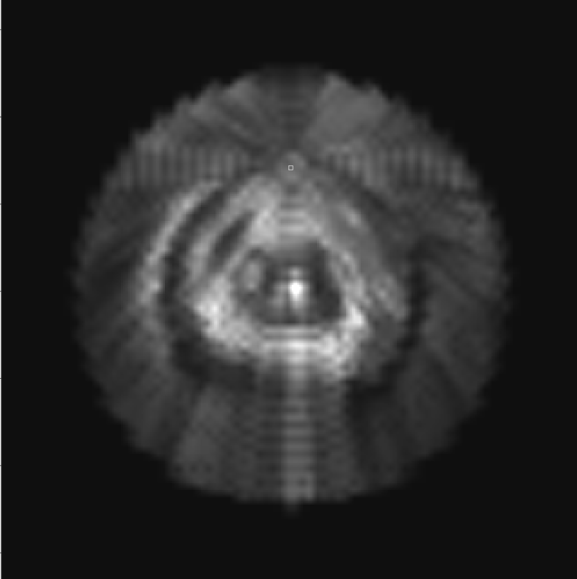
Figure 2: Face-on view of the surface density of gas in the Galaxy. The square indicates the position of the sun. The color scale is linear between surface mass densities of -2 $M_{\odot}\,pc^{-2}$ and 30 $M_{\odot}\,pc^{-2}$. The plot includes atomic, molecular, and ionized gas integrated from -500 pc to 500 pc height above the plane.

For a region of $\sim\,20^{\circ}$ towards the Galactic Center and towards the anticenter the kinematical resolution is insufficient, and the data have been edited by hand. The distribution of gas in these two regions is basically an interpolation between the results for the adjacent regions. In the anticenter region any excess over this interpolation has been evenly distributed over all distances, while in the Galactic Center region any excess is attributed to the Galactic Center. The distribution of gas in the Galactic plane is shown in Fig.2.

3.2 The spatial distribution of sources

The true distribution of SNR in the Galaxy is not well known as a result of selection effects and the absence of a proper distance measure to the remnants. In many papers (Stecker and Jones (1977); Dogiel and Uryson (1988); Bloemen et al. (1993)) the cosmic ray distribution in the Galaxy has been estimated on the basis of a functional form for the SNR distribution which fits the data for 116 remnants (Kodaira (1974)). One of the general findings in these studies is that the overall cosmic ray distribution is too steep to explain the gradual slope of the $\gamma$-ray emissivity over the Galactic radius (Strong et al. (1988); Strong and Mattox (1996)).

Here we use a revised functional form for the SNR distribution (Case and Bhattacharya (1996)), which fits the data for 194 remnants

$$f(r)=\left({{r}\over{r_{\odot}}}\right)^{1.69\pm 0.22}\exp\left(-(3.33\pm 0.37){{r-r_{\odot}}\over{r_{\odot}}}\right)$$ (20)

where $r_{\odot}=$8.5 kpc denotes the distance between the sun and the Galactic Center. The vertical distribution of SNR is taken to be box-shaped with a half thickness of 150 pc.

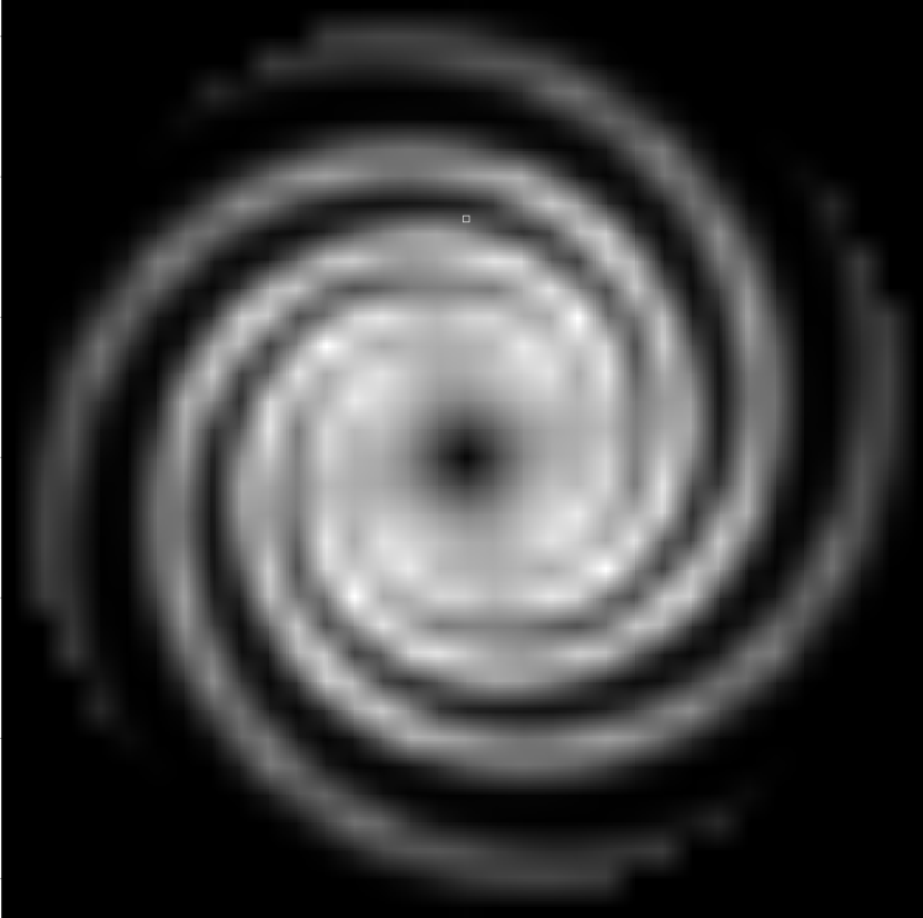
Figure 3: Face-on view of the SNR distribution in the Galaxy according to the spiral arm model. The square indicates the position of the sun. The color scale is linear between zero and peak value. Note that the sun is located in an interarm region.

Our model allows us to use true 3D source distributions. We know that the Galaxy has structure in the form of spiral arms, a bulge and so forth. We have thus folded a spiral arm model (Georgelin and Georgelin (1976); Vallée (1995)) with the radial SNR distribution as described above to investigate the influence of spiral arm structure. In the Georgelin and Georgelin model the Galaxy has four symmetric arms with pitch angle of around 12^∘. We have rescaled their model to $r_{\odot}=$8.5 kpc. Each spiral arm is described by a Gaussian of dispersion 500 pc, i.e. a FWHM of 1177 pc. The spiral arm model is normalized in azimuth, so that the integral $\smallint_{0}^{2\pi}r\,d\phi$ of that model yields unity, and then folded with the radial SNR distribution. The normalization is required to preserve the radial distribution of SNR. A face-on view of the resultant source distribution is shown in Fig.3.

4 Results

In this section we show results for two choices of the spatial distribution of sources, the pure SNR distribution and the SNR distribution folded with a model of the spiral arms in the Galaxy. We will also show results for two choices of injection index, at first a fixed index s=2.0 for all sources, and then a normal distribution of indices with mean 2.0 and dispersion 0.2. We will not vary any other parameter in the propagation model, and stick to the best fit values given by Webber, Lee and Gupta (1992). In a forthcoming paper we will extend our model to nucleons and determine the propagation parameters self-consistently which fit the $\gamma$-ray data and the local spectra of primary and secondary cosmic rays. In this paper our emphasis is to show that an injection index of around s=2.0 for cosmic ray electrons is sufficient to explain the observed spectrum of diffuse high-energy $\gamma$-rays , while leaving all other parameters unchanged.

4.1 The local electron spectra

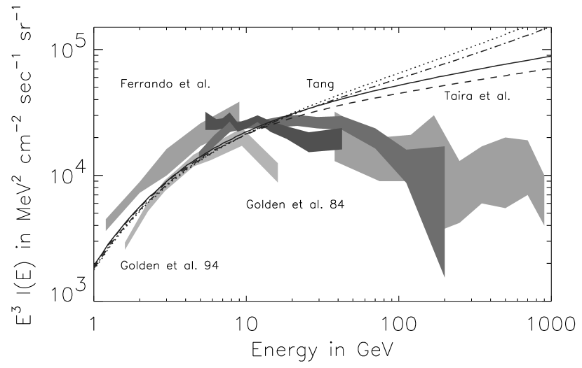
Figure 4: The data for the local flux of cosmic ray electrons compared with the steady state model spectrum. Solar modulation is taken into account using a force-field parameter $\Phi=400\,{\rm MV}$ (Gleeson and Axford (1968)). For the case of the pure SNR distribution as electron source distribution, the solid line is for sources with fixed injection index s=2.0, while the dotted line is for source indices with a normal distribution of mean 2.0 and dispersion 0.2. When the SNR distribution in spiral arms is taken as source distribution, we obtain the dashed line for sources with fixed injection index s=2.0 and the dash-dotted line for source indices with a normal distribution of mean 2.0 and dispersion 0.2.

We have shown in Sec.2 that if electrons are accelerated in SNR, their local spectra above $\sim$ 30 GeV will strongly depend on time, so that the direct electron measurements above this energy may deviate from the average electron spectrum. As a result, we are not required to choose the electron injection index according to the directly observed electron spectrum above $\sim$ 30 GeV. Below a few GeV, on the other hand, the locally observed spectra are strongly affected by solar modulation, for which we do not have reliable models, so that only over roughly one decade in energy does the local electron spectrum provide clear data. The data from direct electron measurements compared with the steady-state spectra of our model are shown in Fig.4. The model spectra fit the data reasonably well in the relevant energy range up to 30 GeV.

4.2 The $\gamma$-ray emission

As an example we show in Fig.5 the spectra of the bremsstrahlung and inverse Compton emission in the direction of the inner Galaxy for the case of sources with injection indices following a normal distribution of mean s=2.0 and dispersion $\mu$=0.2. The figure includes the results of our model, the observed spectrum, and a template of the $\pi^{0}$-decay spectrum (Dermer (1986)). At around 5 GeV the intensity due to leptonic processes is higher than that due to hadronic $\pi^{0}$ decay. Our model assumes that the power-law behaviour of the electron injection spectra persists to $\sim$20 TeV. The high-energy $\gamma$-ray spectrum will rather directly reflect structure in the electron source spectra. If for example the true source spectrum would deviate from a simple power-law above 1 TeV, the Inverse Compton spectrum would show corresponding features above 50 GeV.

When we consider the latitude distribution of the $\gamma$-ray intensity above 1 GeV, which is done in Fig.6, we find a high level of agreement. The fraction of the total diffuse intensity, which is due to leptonic emission, is almost constant between b=0^∘ and b=10^∘. It goes up from $\sim$6% in the Hunter et al. model, $\sim$10% in our model for an injection index of s=2.4, to 30% - 48% for an injection index of s=2.0, enough to explain all the $\gamma$-ray excess.

We can compare the longitude distribution of the observed diffuse $\gamma$-ray emission above 1 GeV to that of the leptonic contribution in our model. This is done in Fig.7. It is obvious that the galactocentric gradient of the leptonic $\gamma$-ray emission in our model is stronger than in the data. This is the case for all cosmic ray propagation models which are based on the SNR distribution (Webber, Lee and Gupta (1992); Bloemen et al. (1993)). While towards the inner Galaxy the fraction of the total diffuse intensity, which is due to leptonic emission, is around 35% - 52%, far enough to explain all the $\gamma$-ray excess, towards the outer Galaxy the leptonic contribution in our model accounts only for roughly two thirds of the excess.

The SNR distribution of Case and Bhattacharya has a zero at galactocentric radius r=0 which causes the double peak structure in the model intensity towards the inner Galaxy. Such double peak structure is not visible in the data, so that this effect may result more from the specific choice of mathematical function in the fit of the SNR distribution than astrophysical reality. We can generally say that a flatter SNR distribution would beget a better harmony of the longitude distribution of observed emission and model. Interestingly, one study of the SNR distribution, which was not based on a specific form of the radial profile, indicates very long radial scale lengths up to 9 kpc (Li et al. (1991)).

We have therefore investigated the impact of the fit uncertainties in the SNR distribution. Within 1 $\sigma$ in both parameters the SNR distribution may be

$$f(r)=\left({{r}\over{r_{\odot}}}\right)^{1.91}\exp\left(-2.96{{r-r_{\odot}}\over{r_{\odot}}}\right)$$ (21)

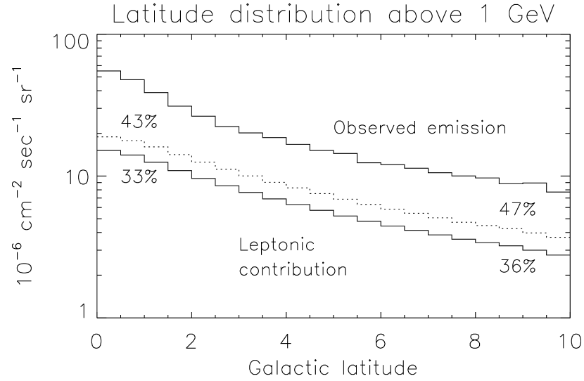
Figure 8: The latitude distribution of the $\gamma$-ray emission above 1 GeV as in Fig.6 except that here the flatter SNR distribution in spiral arms has been used. The indicated percentage of leptonic contribution of 33% - 47% is sufficient to account for all the excess.

Here we show the results for the spiral arm model only. For similar local electron spectra the leptonic contribution to the diffuse Galactic $\gamma$-ray emission above 1 GeV can be 33% -47% while the center/anticenter contrast in the model agrees with the observed one to better than 25%. As can be seen in Fig.8, the latitude distribution of the leptonic contribution varies little. The longitude distribution of the leptonic contribution in Fig.9 shows that the overall gradient is reasonably well reproduced, but the double hump structure towards the inner Galaxy remains as well as a general overprediction around $|l|\approx 45^{\circ}$. This double hump structure however is a consequence of the mathematical function chosen to fit the SNR distribution and not a consequence of the SNR distribution itself.

4.3 The synchrotron emission

A further constraint on our model is the synchrotron flux towards the North Galactic Pole (NGP). Available data at 408 MHz (Haslam et al. (1982)), at 820 MHz (Berkhuijsen (1972)), and at 1420 MHz (Reich and Reich (1986)) can be corrected for zero level uncertainties, the contributions of the microwave background and unresolved extragalactic sources (Reich and Reich (1988)), and contributions from the Coma cluster (Schlickeiser, Sievers and Thiemann (1986)). Here we do not use data at frequencies below 100 MHz, which we expect to be affected by free-free absorption. In Fig.10 we compare the synchrotron intensity predicted by our model with the data in direction of the NGP. It can be seen that for a total magnetic field strength of 10$\mu$G there is good agreement.

In our model the FWHM of the z-distribution of synchrotron emission at 1420 MHz is $\sim$1.1 kpc, which is the value typically found for edge-on galaxies (Hummel (1991)).

5 Summary and discussion

In this paper we have investigated whether cosmic ray electrons can be responsible for the recently observed high intensity of diffuse Galactic $\gamma$-ray emission above 1 GeV. Models based on the locally observed cosmic ray spectra underpredict the observed intensity by nearly 40% (Hunter et al. (1997)). One feature of these models is the relatively soft electron injection spectral index of s=2.4 (Skibo (1993)), which is required to account for the local electron spectrum above 50 GeV.

The recent detection of non-thermal X-ray synchrotron radiation from the four supernova remnants SN1006 (Koyama et al. (1995)), RX J1713.7-3946 (Koyama et al. (1997)), IC443 (Keohane et al. (1997)), and Cas A (Allen et al. (1997)) supports the hypothesis that Galactic cosmic ray electrons are accelerated predominantly in SNR. We have shown in this paper that, if this is indeed the case, the local electron spectra above 30 GeV are variable on time scales of a few hundred thousand years. This variability stems from the Poisson fluctuations in the number of SNR in the solar vicinity within a certain time period. While the electron spectra below 10 GeV are stable, the level of fluctuation increases with electron energy, and above 100 GeV the local electron flux is more or less unpredictable.

With that time variability in mind we have seen that an electron injection index of s=2.0 is consistent with the data of the direct particle measurements if SNR are the dominant source of cosmic ray electrons. In fact, both the radio spectra of individual SNR (Green (1995)) and the hard spectrum of the inverse Compton emission at high latitudes (Chen, Dwyer and Kaaret (1996)) would better harmonize with an injection index of s=2.0 instead of s=2.4.

We have then presented a three-dimensional steady-state diffusion model for cosmic ray electrons, based on the propagation parameters which have been derived from similar models for cosmic ray nucleons. While being entirely consistent with the local electron electron flux up to $\sim$ 30 GeV energy and with the radio synchrotron spectrum towards the North Galactic Pole, the leptonic contribution to the diffuse Galactic $\gamma$-ray emission above 1 GeV in the Galactic plane increases from $\sim$6% in the model of Hunter et al., $\sim$, 10% in our model for an injection index s=2.4, to 30-48% for an injection index s=2.0 depending on the assumed spatial distribution of SNR and depending on whether some dispersion of injection spectral indices is allowed. An electron injection index s=2.0 can therefore explain the bulk of the observed $\gamma$-ray excess over the predictions of the Hunter et al. model.

While the latitude distribution of the leptonic $\gamma$-ray emission is fully consistent with that of the observed emission, we find that the longitude distribution deviates from the observed one. In our model the contrast between the Galactic Center and the anticenter is stronger than in the data. A similar effect can be found in all cosmic ray propagation models which are based on the SNR distribution (Webber, Lee and Gupta (1992); Bloemen et al. (1993)). Note that in the Hunter et al. model only the emissivity spectrum is taken according to a propagation calculation (Skibo (1993)), while the spatial distribution of the emissivity is scaled according to the distribution of thermal gas.

We have seen that the fit uncertainties in the SNR distribution of Case and Batthacharya allow us to use a flatter profile, which leads to a better agreement between model and data in the longitude distribution (see Fig.9). Thus the gradient problem may be simply the result of an inappropriate choice of radial SNR distribution or lack of error propagation, respectively. This flatter profile would also harmonize better with the results of Li et al. (1991), who found very large radial scale lengths of up to 9 kpc for the galactic distribution of SNR. Other possible sources of systematic errors are discussed below.

This gradient problem is unlikely to be caused by additional thermal matter. Very cold (3^∘K) molecular gas has recently been discussed as candidate for baryonic dark matter (Pfenniger et al. (1994)). If organised in small clumps (Pfenniger and Combes (1994)) the probability of finding absorption features in the spectra of bright background objects would be small and the clumps would easily evade detection (for a review see Combes and Pfenniger (1997)). However, the thermal gas mainly affects the bremsstrahlung and only indirectly the inverse Compton emission, which dominates above 1 GeV $\gamma$-ray energy, and thus has little influence on the gradient in the total leptonic $\gamma$-ray emission above 1 GeV.

If our model for the interstellar radiation field were wrong, then it would have only a limited influence on the gradient, since the Galaxy acts as a fractional calorimeter at high electron energies (Pohl (1994)), which channels the electron source power directly into synchrotron and inverse Compton emission with a ratio corresponding to that of the energy densities in the magnetic field and the photon field. Any radial variation of the magnetic field strength will be directly reflected in the Center/anticenter contrast of the synchrotron intensity, so that the radio surveys would constrain the parameter space here.

It is our personal view that the uncertainties in the radial distribution of SNR are large enough so that the overly strong gradient in our model may simply be the result of an inappropriate choice of SNR distribution. The artificial double peak structure towards the inner Galaxy is an example of systematic effects which arise from possibly ill-defined fits to the SNR distribution.

Our findings indicate a potential problem in the determination of the extragalactic $\gamma$-ray background (Sreekumar et al. (1998)). The standard method uses a linear regression analysis of observed intensities and model predictions (with the model of Hunter et al.) to extrapolate to zero Galactic intensity. If at higher $\gamma$-ray energies the inverse Compton emission is indeed much stronger than assumed by Hunter et al., then a large fraction of it will be attributed to the extragalactic $\gamma$-ray emission. Our steady-state model predicts an intensity of high-latitude inverse Compton emission above 1 GeV at a level of $\sim 40\%$ of the extragalactic background intensity, while Hunter et al. assume much smaller values. The intensity difference between the inner Galaxy and the outer Galaxy at medium latitudes ($40^{\circ}-50^{\circ}$) would be around 10% of the extragalactic background intensity, depending on the choice of model for the electron source distribution (SNR distribution). On the other hand, if we are indeed living in a region of temporarily low flux of high-energy electrons, we would also expect the intensity of inverse Compton emission towards the Galactic Poles to be less that the steady-state value, so that the true level of Galactic $\gamma$-ray intensity at high latitudes is difficult to assess.

The spectrum of inverse Compton emission, s$\simeq$1.85 in our model, is somewhat harder than the s$\simeq$2.1 of the extragalactic background. It has been noted before that the average $\gamma$-ray spectrum of the identified AGN is softer than that of the background (Pohl et al. 1997b ), which indicates a problem with the idea that the background is mainly due to unresolved AGN. Now, since the presently determined background spectrum may be substantially contaminated with hard inverse Compton emission, the true background spectrum may be softer than s=2.1, which would probably relieve the spectral discrepancy with the average spectrum of resolved AGN (Pohl et al. 1997b ). Anyway, the systematic uncertainty in the spectral index of the extragalactic $\gamma$-ray background emission is much higher than the statistical uncertainty.

In a forthcoming paper we shall discuss the distribution of synchrotron emission in more detail. We shall also use a truly three-dimensional calculation of the interstellar photon fields based on COBE/FIRAS data. Finally we shall discuss cosmic ray nucleons in parallel with electrons to derive the propagation parameters self-consistently.

Figure 1: The locally observed electron spectra in the upper panel compared with the range of possible spectra in our model. The parameters of the model are given in the main text. For each experiment the 1 $\sigma$ uncertainty range is indicated by a grey-shaded band which connects the data points at the mean energies of the corresponding energy bins. The scatter between the results of different experiments indicates the level of systematic uncertainties. The range of possible spectra in our model is given by the grey-shaded bands in the lower panel. During 68% of the time the locally observed spectra will be in the dark grey shaded region, and during 95% of the time they will be within the light grey shaded region. The dashed black curve gives the 68% range for a weaker energy dependence of the diffusion coefficient (a=0.33 instead of a=0.6) to show the influence of this parameter. The white dash-dotted line shows one of the 400 random spectra as a particular example of what may be observed. The white dotted line indicates the time-averaged spectrum. The effect of solar modulation is taken into account for all model spectra using a force-field parameter $\Phi=400\ {\rm MV}$ (Gleeson and Axford (1968)). The data are not in conflict with the range of possible spectra in our model.

Figure 5: The $\gamma$-ray intensity in the direction of the inner Galaxy. The data points are taken from Hunter et al. (1997). The error bars include an estimate for the systematic error of 8%, which accounts for the uncertainty in the energy-dependent correction of the spark chamber efficiency (Esposito et al. (1998)). The data are compared with bremsstrahlung (ebr) and Inverse Compton (ic) spectra from our model, here on the basis of sources with injection indices following a normal distribution of mean 2.0 and dispersion 0.2 and the spatial distribution of SNR in spiral arms. The $\pi^{0}$-component is a template and not a model.

Figure 6: The latitude distribution of the $\gamma$-ray emission above 1 GeV compared with the model prediction for the leptonic contribution. Again the solid line is for fixed injection index, and the dotted line is for a distribution of indices with dispersion 0.2. The numbers give the percentage of the observed emission in certain directions which is due to leptonic processes. The top panel displays results for the pure SNR distribution as electron source distribution, while the bottom panel is for a source distribution of SNR in spiral arms.

Figure 7: The longitude distribution of the $\gamma$-ray emission above 1 GeV. The upper solid line shows the observed distribution according to Hunter et al. (1997). The distribution of the leptonic emission in our model is shown for comparison, here for the SNR distribution as source distribution. Again the solid line is for fixed injection index, and the dotted line is for a distribution of indices with dispersion 0.2. The numbers give the percentage of the observed emission in certain directions which is due to leptonic processes. The top panel is for the pure SNR distribution and the bottom panel is for a source distribution of SNR in spiral arms.

Figure 9: The longitude distribution of the $\gamma$-ray emission above 1 GeV as in Fig.7 except that here the flatter SNR distribution in spiral arms has been used. The overall gradient is well reproduced. The double hump structure towards the inner Galaxy and the overprediction around $|l|\approx 45^{\circ}$ indicate that the mathematical profile in the fit to the SNR distribution may be ill-defined.

Figure 10: The synchrotron intensity in the direction of the North Galactic Pole. The error bars indicate data from surveys with reasonable zero level calibration. The solid line is the model spectrum based on the pure SNR source distribution while the dotted line is for the SNR distributed in spiral arms.

References

- Allen et al. (1997) Allen G.E. et al., 1997, ApJ, 487, L97
- Arimoto et al. (1996) Arimoto N, Sofue Y., Tsujimoto T., 1996, PASJ, 48, 275
- Barwick et al. (1997) Barwick S.W. et al., 1997, ApJ, 482, L191
- Berkey and Shen (1969) Berkey G.B., Shen C.S., 1969, Physical Review, 188, 1994
- Berkhuijsen (1972) Berkhuijsen E.M., 1972, A&AS, 5, 263
- Bertsch et al. (1993) Bertsch D.L. et al., 1993, ApJ, 416, 587
- Blandford and Eichler (1987) Blandford R., Eichler D., 1987, Phys. Rep., 154, 1
- Bloemen (1989) Bloemen H., 1989, ARA&A, 27, 469
- Bloemen et al. (1993) Bloemen H. et al., 1993, A&A, 267, 372
- Bonino (1996) Bonino G., 1996, Proc. 24th ICRC, Il nuovo cimento Vol. 19C, N.6, p.865
- Brecher and Burbidge (1972) Brecher K., Burbidge G.R., 1972, ApJ, 174, 253
- Buckley et al. (1998) Buckley J.H. et al., 1998, A&A, 329, 639
- Burton (1985) Burton W.B., 1985, A&AS, 62, 365
- Burton (1976) Burton W.B., 1976, ARA&A, 14, 275
- Burton and Liszt (1983) Burton W.B., Liszt H.S., 1983, A&AS, 52, 63
- Case and Bhattacharya (1996) Case G., Bhattacharya D., 1996, A&AS, 120, C437
- Cappelaro et al. (1997) Cappelaro E. et al., 1997, A&A, 321, 431
- Chen, Dwyer and Kaaret (1996) Chen A., Dwyer J., Kaaret P., 1996, ApJ, 463, 169
- Cleary, Heiles and Haslam (1979) Cleary M.N., Heiles C., and Haslam C.G.T, 1979, A&AS, 36, 95
- Clemens (1985) Clemens D.P., 1985, ApJ, 295, 422
- Combes and Pfenniger (1997) Combes F., Pfenniger D., 1997, A&A, 327, 453
- Cowsik and Lee (1979) Cowsik R., Lee M.A.: 1979, ApJ, 228, 297
- Dame et al. (1987) Dame T.M. et al., 1987, ApJ, 322, 706
- Dermer (1986) Dermer C.D., 1986, A&A, 157, 223
- Digel and Dame (1997) Digel S.W., Dame T.M., 1997, private communication
- Digel et al. (1996) Digel S.W. et al., 1996, ApJ, 463, 609
- Digel et al. (1995) Digel S.W., Hunter S.D., Mukherjee R., 1995, ApJ, 441, 270
- Dogiel and Uryson (1988) Dogiel V.A., Uryson A.V., 1988, A&A, 197, 335
- Drury, Aharonian and Völk (1994) Drury L. O’C., Aharonian F.A., Völk H.J., 1994, A&A, 287, 959
- Esposito et al. (1998) Esposito J.A. et al., 1998, ApJ, submitted
- Fazio et al. (1966) Fazio G.G., Stecker F.W., Wright J.P., 1966, ApJ, 144, 611
- Ferrando et al. (1996) Ferrando P. et al., 1996, A&A, 316, 528
- Fichtel et al. (1975) Fichtel C.E. et al., 1975, ApJ, 198, 163
- Gleeson and Axford (1968) Gleeson L.J., Axford W.I., 1968, ApJ, 154, 1011
- Georgelin and Georgelin (1976) Georgelin Y.M., Georgelin Y.P., 1976, A&A, 49, 57
- Ginzburg and Syrovatskii (1964) Ginzburg V.L., Syrovatskii S.I.: 1964, The origin of cosmic rays, Pergamon Press
- Golden et al. (1994) Golden R.L. et al., 1994, ApJ, 436, 769
- Golden et al. (1984) Golden R.L. et al., 1984, ApJ, 287, 622
- Green (1995) Green D.A., 1995, ’A catalogue of Galactic SNR’, Mullard RAO, Cambridge, UK
- Hammersley et al. (1995) Hammersley P.L. et al., 1995, MNRAS, 273, 206
- Haslam et al. (1982) Haslam C.G.T. et al., 1982, A&AS, 47, 1
- Heiles and Habing (1974) Heiles C., Habing H.J., 1974, A&AS, 14, 557
- Hummel (1991) Hummel E., 1991, IAU Symposium 144, Ed. H. Bloemen, Kluwer, p.257
- Hunter et al. (1997) Hunter S.D. et al., 1997, ApJ, 481, 205
- Hunter et al. (1994) Hunter S.D. et al., 1994, ApJ, 436, 216
- Keohane et al. (1997) Keohane J.W. et al., 1997, ApJ, 484, 350
- Kerr et al. (1986) Kerr F.J. et al., 1986, A&AS, 66, 373
- Kocharov (1996) Kocharov G.E., 1996, Proc. 24th ICRC, Il nuovo cimento Vol. 19C, N.6, p.883
- Kodaira (1974) Kodaira K., 1974, PASJ, 26, 255
- Koyama et al. (1997) Koyama K. et al., 1997, PASJ, 49, L7
- Koyama et al. (1995) Koyama K. et al., 1995, Nature, 378, 255
- Kraushaar et al. (1972) Kraushaar W. et al., 1972, ApJ, 177, 341
- Lerche and Schlickeiser (1981) Lerche I., Schlickeiser R., 1981, ApJS, 47, 33
- (54) Lerche I., Schlickeiser R., 1982, MNRAS,. 201, 1041
- (55) Lerche I., Schlickeiser R., 1982, A&A, 107, 148
- Lessard et al. (1995) Lessard R.W. et al., 1995, 24th ICRC, 2, 475
- Li et al. (1991) Li Z., Wheeler J.C., Bash F.N., Jefferys W.H., 1991, ApJ, 378, 93
- Mayer-Hasselwander et al. (1982) Mayer-Hasselwander H. et al., 1982, A&A, 105, 164
- McHargue, Damon and Donahue (1995) McHargue L.R., Damon P.E., Donahue D.J., 1995, Geoph. Res. Lett., 22, 659
- McLaughlin et al. (1996) McLaughlin M.A. et al., 1996, ApJ, 473, 763
- Merck et al. (1996) Merck M. et al., 1996, A&AS, 120, C465
- Mori (1997) Mori M., 1997, ApJ, 478, 225
- Pfenniger and Combes (1994) Pfenniger D., Combes F., 1994, A&A, 285, 94
- Pfenniger et al. (1994) Pfenniger D., Combes F., Martinet L., 1994, A&A, 285, 79
- Pohl (1996) Pohl M., 1996, A&A, 307, L57
- Pohl (1994) Pohl M., 1994, A&A, 287, 453
- Pohl and Schlickeiser (1990) Pohl M., Schlickeiser R., 1990, A&A, 234, 147
- (68) Pohl M., Kanbach G., Hunter S.D., Jones B.B., 1997a, ApJ, 491, 159
- (69) Pohl M., Hartman R.C., Jones B.B., Sreekumar P., 1997b, A&A, 326, 51
- Porter and Protheroe (1997) Porter T.A., Protheroe R.J., 1997, J. Phys. G, 23, 1765
- Reich and Reich (1986) Reich P., Reich W., 1986, A&AS, 63, 205
- Reich and Reich (1988) Reich P., Reich W., 1988, A&AS, 74, 7
- Schlickeiser et al. (1997) Schlickeiser R., Pohl M., Ramaty R., Skibo J.G., 1997, Proc. 4th Compton Symposium, Eds. C.D. Dermer and J.D. Kurfess, AIP Conf. Proc. 410, p.449
- Schlickeiser (1982) Schlickeiser R., 1982, A&A, 106, L5
- Schlickeiser, Sievers and Thiemann (1986) Schlickeiser R., Sievers A., Thiemann H., 1987, A&A, 182, 21
- Skibo (1993) Skibo J.G., 1993, PhD dissertation, University of Maryland
- Sodroski et al. (1995) Sodroski T.J. et al., 1995, ApJ, 452, 262
- Sonnett et al. (1987) Sonnett C.P. et al., 1987, Nature, 330, 458
- Sreekumar et al. (1993) Sreekumar P. et al., 1993, Phys. Rev. Lett., 70, 127
- Sreekumar et al. (1998) Sreekumar P. et al., 1998, ApJ, 494, 523
- Stecker and Jones (1977) Stecker F.W., Jones F.C., 1977, ApJ, 217, 843
- Strong (1997) Strong A.W., 1997, private communication
- Strong and Mattox (1996) Strong A.W., Mattox J.R., 1996, A&A, 308, L21
- Strong (1995) Strong A.W., 1995, Space Sci. Rev., 76, 205
- Strong et al. (1988) Strong A.W. et al., 1988, A&A, 207, 1
- Taira et al. (1993) Taira T. et al., 1993, 23rd ICRC, 2, 128
- Tang (1984) Tang K.K., 1984, ApJ, 278, 881
- Tanimori et al. (1997) Tanimori T. et al., 1997, IAUC 6706
- Taylor and Cordes (1993) Taylor J.H., Cordes J.M., 1993, ApJ, 411, 674
- Vallée (1995) Vallée J.P., 1995, ApJ, 454, 119
- Weaver and Williams (1973) Weaver H.F., Williams D.R.W., 1973, A&AS, 8,1
- Webber, Lee and Gupta (1992) Webber W.R., Lee M.A., Gupta M., 1992, ApJ, 390, 96
- Webster (1970) Webster A.S., 1970, Astrophys. Lett., 5, 189
- Youssefi and Strong (1991) Youssefi G., Strong A.W., 1991, 22nd ICRC, 1, 129