Modelling emission line profiles of a non–uniform accretion disk

Abstract

Techniques of calculation of emission line profiles formed in a non–uniform accretion disk is presented. Change of the profile shape as a function of phase turn of the disk with a bright spot on the surface is analysed. A possibility of a unambiguous determination of the disk and spot parameters is considered, the accuracy of their determination is estimated. The results of calculations show that the analysis of spectra obtained at different phases of the orbital period gives a possibility of estimating the basic parameters of the spot (such as geometric size and luminosity) and to investigate the structure of the accretion disk.

Key words:   accretion – accretion disks – lines: formation – lines: profile – methods: numerical

1 Introduction

By the present time a large number of close binary systems containing a component with an accretion disk have been detected. In such systems a secondary nondegenerate star fills its critical Roche lobe and transfers matter to the primary star through the inner Lagrangian point mostly as a gas stream. Due to the high angular momentum the outflowing gas forms the accretion disk around the primary “peculiar” component. At the place the gas stream strikes the outer rim of the disk an area of enhanced temperature and luminosity, named bright spot, is formed.

In Algol–type systems the disk accretion occurs on a normal B–A main–sequence star (Plavec, 1980), and in cataclysmic variables and X–ray binaries it occurs on a degenerate star (Kraft, 1965). In the last case the accretion disk may give an appreciable contribution to the optical continuum (Pringle and Rees, 1972; Shakura and Sunyaev, 1973).

Cataclysmic variables are the most suitable objects for the study of accretion disks. These close binary systems consist of a white dwarf (primary) and a main–sequence star of a late spectral class (G–M). The choice of cataclysmic variables for research into accretion disks is defined by the following factors:

1. The main part of energy radiation from the disk is emitted at optical and ultraviolet wavelengths;

2. The contribution of the secondary component (a star of the late spectral type G–K) to the system total luminosity is relatively small in comparison with that of the accretion disk;

3. Cataclysmic variables are usually more amenable to observations than low–mass X–ray binaries. This makes it definitely easier to get observational data of high quality;

4. The number of cataclysmic variables is much greater than the number of representatives of other types of binaries with accretion disks.

Typical optical spectra of cataclysmic variables contain emission lines of hydrogen, neutral helium and singly ionized calcium all superposed onto a blue continuum. He II 4686 may also be present. In the spectra of systems with high inclinations the emission lines of H and He I are usually double–peaked and have profiles with base widths over 2000–3000 km/s (Williams, 1983; Honeycutt et al., 1987).

The double–peaked profile is a result of Doppler shift of emission from the accretion disk (Smak, 1969; Horne and Marsh, 1986). The profiles are often observed to be asymmetric and the intensities of the red and blue peaks are variable with the orbital period phase (Greenstein and Kraft, 1959). The trailed spectra show strong double–peaked symmetrical line profiles and a weak narrow component which forms a S–wave due to sinusoidal variations of its radial velocity. The “S-wave” component is usually attributed to the bright spot — the point of interaction of the gas stream and the accretion disk (Kraft, 1961; Smak, 1976), moreover their physical parameters define the nature of the processes involved (Livio, 1992). This makes it important to study the observational properties in the investigation of accretion in close binary systems.

In this paper we consider a method of modelling emission line profiles which are formed in non-uniform accretion disks. We study the line profile variation depending on the phase turn of the disk with the bright spot on the surface. In section 2 the model and the technique of calculations are described. In section 3 we test this method for the determination of the line profile from the model parameters. Evaluation of the accuracy of determination of parameters is described in section 4. Finally, in section 5 the results of calculations are given.

2 Method

A powerful tool in the investigation of the orbital variations of emission lines in spectra of close binaries, which is widely used now, is Doppler tomography. This is an indirect imaging technique which can be used to determine the two–dimensional velocity-field distribution of line emission in binary systems (Marsh and Horne, 1988). This method provides very accurate reconstructions even when analyzing low S/N–ratio spectra. However, such a powerful tool in studying the structure of accretion disks is unfortunately not free from demerits. We point out only the basic of them.

• The computation of a Doppler map requires a large number of high resolution spectra covering an orbital period. This is a problem when studying weak and short–period close binary systems.

• The variation in flux of the disk details during observations may distort the map (Marsh and Horne, 1988). This occured, for example, in the study of the cataclysmic variable U Gem (Marsh et al., 1990). In the Doppler map the ring–shaped component from the disk is weakened near the bright spot. This weakening is actually non–existent.

• Since all the observational data are used for computation of the map, we lose the possibility of studying variations of fluxes from the bright spot and other emission regions over the orbital period.

The enumerated shortcomings of the method of Doppler tomography restrict possibilities of its use. The modelling of the line profiles obtained at different phases of the orbital period is another possible method of analysis of variations of the accretion disk and spot parameters with time, without mapping the disk in the velocity field. Thus, at a sacrifice the high spatial resolution we obtain a possibility of studying the temporal variability.

For accurate calculation of line profiles formed in the accretion disk, it is necessary to know the velocity field of radiating gas, its temperature and density, and, first of all, to calculate the radiative transfer equations in lines and the balance equations. Unfortunately, this complicated problem has not been solved until now and it is still not possible to reach an acceptable consistency between calculations and observations. Nevertheless, even the simplified models allow one to define some important parameters of the accretion disk.

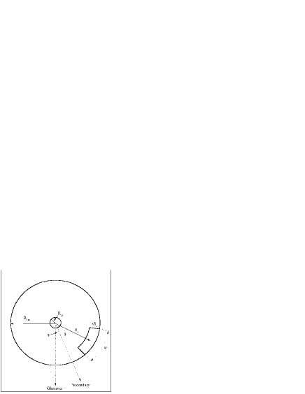
Figure 1: Accretion disk geometry for the line profile model described in the text.

In close binary systems it is possible to note five basic emission regions: an accretion disk, a gas stream, a bright spot, a primary and a secondary components. However, in low–mass systems the accretion disk and the bright spot only make the main contribution to the radiation of emission lines (see, for example, Marsh et al., 1990; Marsh and Horne, 1990). Therefore in our calculations we applied a two–component model which included a flat Keplerian geometrically thin accretion disk and a bright spot whose position is constant with respect to the components of a binary system (Fig. 1). We began the modelling of line profiles with calculation of a symmetrical double–peaked profile formed in a uniform axisymmetrical disk, then we added a distorting component formed in the bright spot.

The flat Balmer line decrement usually observed in spectra of cataclysmic variables shows that the hydrogen emission lines are optically thick. In this case the local emissivity of the lines becomes strongly anisotropic, because the photons tend to emerge easily in the directions of high velocity gradients. Therefore for the calculation of the line profiles we have used the method of Horne and Marsh (1986), taking into account the Keplerian velocity gradient across the finite thickness of the disk. To calculate the emission line profile we divide the disk surface into a grid of elements, and assign the velocity vector, line strength and other parameters for each element. The computation of the profiles proceeds by summing the local line profiles weighted by the areas of the surface elements. For details see Horne and Marsh (1986) and Horne (1995).We have assumed a power–law function for distribution of the local line emissivity $f(r)$ over the disk’s surface $f(r)\propto r^{-\alpha},$ where r is the radial distance from the disk’s centre and $\alpha=1\div 2.5$ (Smak, 1981; Horne and Saar, 1991).

Free parameters of our model are:

1. Parameter $\alpha$;

2. $R=R_{in}$/R_out — the ratio of the inner and the outer radii of the disk;

3. $V$ — radial velocity of the outer rim of the accretion disk.

   Unfortunately, the theoretical modelling of the stream–disk interaction is in its infancy. It is known from photometric and spectral studies that over the orbital period the bright spot is eclipsed by the outer edge of the accretion disk (see, for example, Livio et al., 1986). However, it is still unclear if the spot is optically thick. By the optically thick spot we mean one for which anisotropy of the local line emissivity should be taken into account. We consider this problem in details in the next section. In our model we consider the spot on the accretion disk to have a Keplerian velocity and to be described by four geometric parameters (Fig.1):

4. $A$ — the azimuthal angle of the spot centre relative to the line of sight, $A=\varphi+\vartheta$ (Fig. 1);

5. $\Psi$ — the spot azimuthal extent;

6. $R_{S}$ — the radial position of the spot centre in fractions of the outer radius ($R_{out}$=1);

7. $\Delta R_{S}$ — the radial extent.

   For simplicity we assume that the brightness ratio of the spot and disk is constant and the spot brightness does not depend on azimuth ($f_{S}(A)=const)$, and its dependence on radius is described by the function

8. $f_{S}(r)=B\cdot f(r)\propto B\cdot r^{-\alpha}$, where the free parameter $B$ is the spot brightness. For the further analysis instead of $B$ it is preferable to use the relative dimensionless luminosity $L$, which is determined as

   $\begin{array}[t]{l}L=\int\limits_{R_{S}-\Delta R_{S}/2}^{R_{S}+\Delta R_{S}/2}S\cdot B\cdot f(r)\cdot dr=\\ \\ =\frac{\pi}{180}\frac{\Psi\Delta R_{S}B}{2-\alpha}\left[\left(R_{S}+\frac{\Delta R_{S}}{2}\right)^{2-\alpha}-\left(R_{S}-\frac{\Delta R_{S}}{2}\right)^{2-\alpha}\right]\end{array}$

   where $S$ – the spot area, and $B$ – the spot brightness.

So, our accretion disk model has 8 parameters. Such multiparametric reverse problems raise a question on the uniqueness and stability of the solution. In order to answer it, we analyze how the various parameters of the spot and disk affect a line profile.

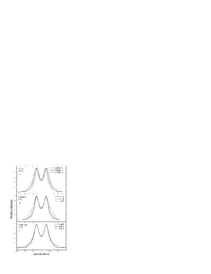
Figure 2: Relationship between the line profile and the accretion disk model parameters: a) V, b) parameter $\alpha$, c) R.

3 Line profile dependence on the model parameters

3.1 Parameters of the accretion disk

The dependence of the line profile on the parameters of the uniform accretion disk is considered in details by Smak (1981) and Horne and Marsh (1986). They have shown that the accretion disk parameters basically affect different parts of line profiles on the whole, and therefore they can be determined unambiguously. Really, the velocity of the outer rim of the accretion disk $V$ defines the distance between the peaks in the lines (Fig. 2a), the shape of the line profile depends on the parameter $\alpha$ (Fig. 2b), and the extent of the wings is determined by $R$ (Fig. 2c).

3.2 Parameters of the bright spot

When we studied the dependence of the emission line profiles on the parameters of the bright spot it was important to find out whether it was possible to make their unambiguous estimates. The results of testing presented below are based on the modelling of a series of line profiles of the accretion disk with the bright spots on different azimuths and having different parameters. Some of them were fixed here, but others were changed so that the relative spot luminosity was constant. The calculations have shown that correct determination of the spot parameters depends on its azimuth, which is necessary to find in an independent way. This is possible from the analysis of the phase variations of asymmetry degree of emission lines (for example, v/r ratio). The azimuth of the spot is $A=\vartheta+\varphi=1+\varphi-\varphi_{0}$, where $\vartheta$ — the phase angle of the spot, $\varphi$ — the orbital phase, and $\varphi_{0}$ — the phase of the moment when the v/r-ratio is equal to 1. It corresponds to the moment when the radial velocity of the S–wave components is zero. Note that in practice to improve the accuracy of measuring the asymmetry degree, instead of the ratio of intensities of the line peaks it is preferable to use the quantity:

$S=\left\{\begin{array}[]{l}\Sigma_{B}/\Sigma_{R}\\ 2-\Sigma_{R}/\Sigma_{B}\end{array}\right.\hskip 28.45274pt\begin{array}[]{r}\Sigma_{B}>\Sigma_{R},\\ \Sigma_{B}<\Sigma_{R}\end{array}$

where S — the degree of asymmetry, $\Sigma_{B}$ and $\Sigma_{R}$ — the integrals of the line intensity of the violet and the red “humps” (or their parts in equal ranges of wavelengths), respectively (Fig. 3). Moreover, such a quantity is more sensitive to changing the spot parameters.

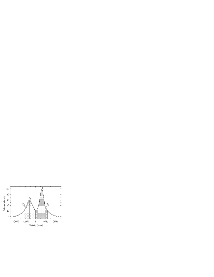
Figure 3: The areas of the “humps”, which are used to increase the accuracy of measuring the asymmetry degree instead of intensities of line peaks (see text for details).

3.2.1 Is the spot optically thin or optically thick?

In an optically thick disk the local line emissivity is strongly anisotropic. Thus the line surface brightness of the accretion disk must be enhanced with non–axisymmetrical pattern and proportional to $\left|sin(2\varphi)\right|$ (Horne and March, 1986; Horne, 1995). This happens because the velocity gradient on spot azimuths $\pm$45^∘ and $\pm$135^∘ is the greatest and the probability of the line photon tending to emerge is also the highest. So, the observed brightness of an optically thick spot will vary with its azimuth (due to its limited size). It will be maximum on azimuths $\pm 45^{\circ}$ and $\pm 135^{\circ}$, fall on the azimuth $\pm 90^{\circ}$ and minimum on azimuths $0^{\circ}$ and $180^{\circ}$. We have calculated a set of models with different parameters of the spot at phases covering the full orbital period, and based on the obtained profiles we have plotted a grid of S–waves (Fig. 4). For the optically thick spot the S–wave curves are seen to have a depression at spot phase $\pm$90^∘. The depth of the depression increases with decreasing azimuth extent of the spot. Such a depression on the S–wave curve may suggest that the spot is optically thick, since in the case of the optically thin spot there is no depression.

Figure 4: Asymmetry degree of the emission line, formed in the accretion disk with the optically thin (a) and optically thick (b) spot as a function of orbital phase.

Figure 5: Spot models used to determine the sensitivity of the line profiles to the spot shape. All the spots have equal relative luminosity and equal area.

3.2.2 The shape of the spot

To find out if the shape of the spot affects the shapes of emission lines, we used the models shown in Fig. 5. In spots of equal relative luminosity and equal area the azimuth extent varied from 10 to 70 degrees. It is seen that the line profile does not depend on the spot shape for azimuth $>45\hbox{${}^{\circ}$}\div 60\hbox{${}^{\circ}$}$ and strongly depends on it at phase $<30\hbox{${}^{\circ}$}\div 45\hbox{${}^{\circ}$}$ (Fig. 6). This is true both for optically thick and optically thin spots.

3.2.3 Radial extent of the spot

Actually the radial extent of the spot does not affect the shape of the line profile. Variation of this parameter over a wide range, from 0.02 to 0.30, affects slightly the profile at all phases and any azimuth extent of the spot. This is explained by the fact that the interval of the radial velocities inside the spot only slightly depends on $\Delta R_{S}$. Therefore it is possible to compensate for the change in this parameter by changing the spot contrast $B$, i.e. the invariant is the product $B\cdot\Delta R_{S}$. So, to calculate the line profile, it is necessary to specify the value of $\Delta R_{S}$ in some way (for example, the typical radial extent of the bright spot). It is known from photometric observations of cataclysmic variables that for different systems it lies in the range $0.02\div 0.15$ (Rozyczka, 1988).

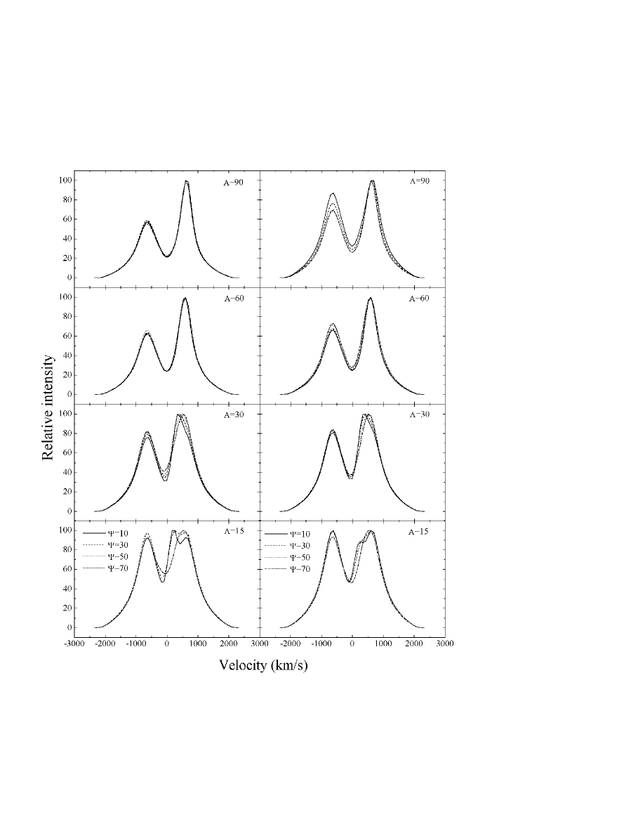
Figure 6: Line profiles as a function of the spot shape. Left — optically thin spot, right — optically thick spot.

3.2.4 Radial position of the spot on the accretion disk

This parameter is determined with high confidence for any optically thick and optically thin spot, which have an azimuth over $45\hbox{${}^{\circ}$}$ (Fig. 7, 8).

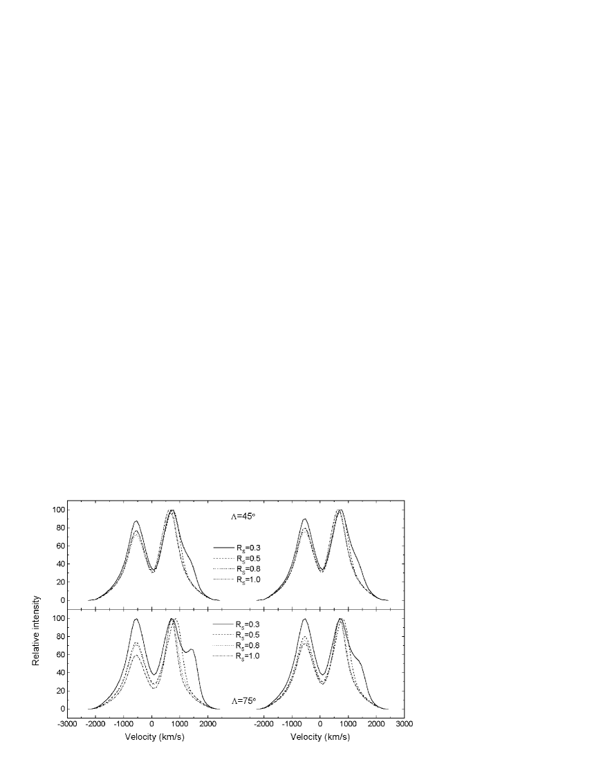
Figure 7: Relationship between the line profile and the radial position of the spot. The parameters of optically thin (left) and of optically thick (right) spots: $\Psi$=70^∘, $\Delta$R_S=0.05.

Figure 8: As in Fig. 7 but the parameters are $\Psi=10^{\circ}$ and $\Delta R_{S}=0.34$.

3.2.5 Radial and azimuthal distributions of the spot brightness

Calculations have shown that the type of the spot brightness distribution does not practically influence the line profile. As an example we adduce the response of the line profile to various types of the azimuth dependence. We have calculated the models with asymmetric distribution of the spot brightness (it is decreasing linearly from $B$ to zero) and with the uniform distribution for comparison. The relative luminosity of the spot was constant. It is seen that the minor modifications of the profile appeared for the spots extended very much in azimuth ($\Psi>70\hbox{${}^{\circ}$}$), at phases close to zero (Fig. 9,10).

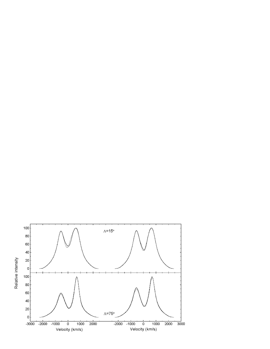
Figure 9: The line profile vs the azimuthal distribution of the spot brightness (solid line — the spot with uniform distribution, dashed line — the spot with asymmetric distribution). The azimuth extent of optically thin (left) and of optically thick (right) spots is $\Psi=70^{\circ}$.

Figure 10: The same as in Fig. 9 but $\Psi=30\hbox{${}^{\circ}$}$.

3.3 Gas stream

The calculation of the line component which is formed in the gas stream has no principal differences from the modelling of the component formed in the bright spot. Because the translational velocity of the stream much exceeds the velocity of its expansion and is highly supersonic, the width of the local line profile formed in the stream must be much smaller than the full width of the line formed in the accretion disk (Lubow and Shu, 1975). Much of the kinetic energy of the stream is released by radiation probably at the moment of its collision with the disk. It is known from observations that usual radii of accretion disks in cataclysmic variables are $(0.4\div 0.8)R_{L}$, where $R_{L}$ is the Roche lobe dimension. The velocity of the stream at such distances from the accreting star approximately corresponds to Keplerian velocities of the accretion disk on these radii. For this reason it is complicated to determine the area of origin of the S–wave component of the observed emission line profile. However this is still possible to do from analysis of the S–wave, for example.

3.4 The secondary component

Research into some dwarf nova (IP Peg, U Gem) using the Doppler tomography technique has shown that secondary components in such systems also contribute to emission in lines (March and Horne, 1990; March et al., 1990). However the contribution of their emission to the total flux is very small and may be ignored in calculations.

4 Evaluation of the accuracy of determination of the parameters

For the further analysis of the obtained results it is important to know the accuracy of determination of the model parameters. It depends on many factors, for example, on the method of determination, on the spectral resolution, and also on the values of the parameters. Because it is nearly impossible to take into account all these factors analytically, we have decided to use the following statistical method. A line profile calculated with the known values of the model parameters was normalized so that the relative intensity of the line was equal to 2 (a value typical of cataclysmic variables). Then the profile was distorted by the Poisson noise (the level of the continuum was varied to change the S/N ratio). After this parameters were fitted to the minimum of residual deviation of a “new” model profile from the “old” noisy one. This procedure was repeated several hundred times, then the average values and the errors of determination of the parameters were estimated. The results of these calculations are shown in Fig. 11. As it can be seen from the plots presented, $V$ and the relative luminosity of the spot are estimated with the highest accuracy. For instance, the accuracy of determination of $V$ under $\rm S/N=30\div 50$ is about 20 km/s. It is better than 5 percent for the typical value of $V$ of about 700 km/s. The parameter $\alpha$ is determined quite confidently. The accuracy of $r$ determination is essentially lower.

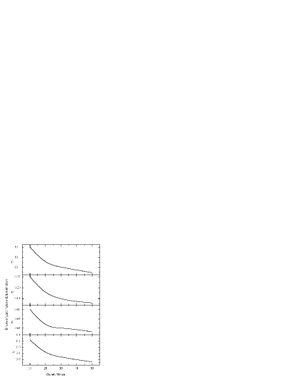
Figure 11: Errors in determination of parameters vs S/N ratio.

5 Conclusions

We have presented a technique for calculation of profiles of emission lines formed in a non–uniform accretion disk. The results of calculations have shown that the analysis of spectra obtained at different phases of the orbital period allows basic parameters of the spot (such as geometric sizes and luminosity) to be estimated and the structure of the accretion disk to be investigated. We have determined that change in the shape of the emission line profiles with the variation of different parameters of the spot strongly depends on the azimuth of the spot. Therefore, the necessary condition for the accurate determination of the parameters of the spot is a knowledge of its phase angle. By separating all spectra according to phases of “the greatest influence” of appropriate parameters we can sequentially determine them.

We have found that:

1. Analysis of the S–wave allows us to determine the phase angle of the spot and its optical depth.

2. The azimuth extent of the spot is determined better on azimuths $<30\hbox{${}^{\circ}$}\div 45\hbox{${}^{\circ}$}$, while its radial position is determined better on azimuths $>50\hbox{${}^{\circ}$}$.

3. The shape of the line profile is practically insensitive to modification in radial extent of the spot. Therefore, for modelling the start value of this parameter is set by default (it is possible to take, for example, a typical radial extent of a bright spot). Thus the number of free parameters of the model decreases by unity.

We thank G.M. Beskin and L.A. Pustil’nik for valuable advice and discussion of the work. The work was partially supported by the Russian Foundation of Basic Research (grant 95-02-03691) and Federal Programme “Astronomy”.

References

- [1] Greenstein J.L., Kraft R.P.: 1959, Astrophys. J., 130, 99
- [2] Honeycutt R.K., Kaitchuck R.H., Schlegel E.M.: 1987, Astrophys. J. Suppl. Ser., 65, 451
- [3] Horne K, Marsh T.R.: 1986, Mon. Not. R. Astron. Soc., 218, 761
- [4] Horne K.: 1995, Astron. Astrophys., 297, 273
- [5] Horne K., Saar S.H.: 1991, Astrophys. J., 374, L55
- [6] Kraft R.P.: 1961, Science, 134, 1433
- [7] Kraft R.P.: 1963, Advances in Astron. and Astrophys., 2, 43
- [8] Livio M.: 1993, Accretion Disks in Compact Stellar Systems, Ed.: Wheeler J.C., World Scientific Publishing Co.
- [9] Livio M., Soker N., Dgani R.: 1986, Astrophys. J., 305, 267
- [10] Lubow S., Shu F.: 1975, Astrophys. J., 198, 383
- [11] Marsh T.R., Horne K.: 1990, Astrophys. J., 349, 593
- [12] Marsh T.R., Horne K. : 1988, Mon. Not. R. Astron. Soc., 235, 269
- [13] Marsh T.R., Horne K., Schlegel E.M., Honeycutt R.K., Kaitchuck R.H.: 1990, Astrophys. J., 364, 637
- [14] Plavec M.J.: 1980, Close Binary Stars: Observations and Interpretation, Eds.: Plavec M.J., Popper D.M. and Ulrich R.K., Dordrecht, Reidel, 155
- [15] Pringle J., Rees M.: 1972, Astron. Astrophys., 21, 1
- [16] Rozyczka M.: 1988, Acta Astron., 38, 175
- [17] Shakura N.I., Sunyaev R.A.: 1973, Astron. Astrophys., 24, 337
- [18] Smak J.: 1969, Acta Astron., 19, 155
- [19] Smak J.: 1976, Acta Astron., 26, 277
- [20] Smak J.: 1981, Acta Astron., 31, 395
- [21] Williams G.: 1983, Astrophys. J. Suppl. Ser., 53, 523