Line Emission from an Accretion Disk Around a Black Hole: Effects of Disk Structure.

Abstract

The observed iron $K\alpha$ fluorescence lines in Seyfert I galaxies provide strong evidence for an accretion disk near a supermassive black hole as a source of the line emission. These lines serve as powerful probes for examining the structure of inner regions of accretion disks. Previous studies of line emission have considered geometrically thin disks only, where the gas moves along geodesics in the equatorial plane of a black hole. Here we extend this work to consider effects on line profiles from finite disk thickness, radial accretion flow and turbulence. We adopt the Novikov & Thorne (1973) solution, and find that within this framework, turbulent broadening is the dominant new effect. The most prominent change in the skewed, double-horned line profiles is a substantial reduction in the maximum flux at both red and blue peaks. The effect is most pronounced when the inclination angle is large, and when the accretion rate is high. Thus, the effects discussed here may be important for future detailed modeling of high quality observational data.

1 Introduction

The Advanced Satellite for Cosmology and Astrophysics (ASCA) has provided data from over a dozen Seyfert I galaxies to reveal the presence of iron emission lines which are broadened by a considerable fraction of the speed of light — greater than 0.2 $c$ in some cases (Mushotzky et al. 1995; Tanaka et al. 1995; Nandra et al. 1997). The observed line profiles are the most direct evidence for the presence of supermassive ($\sim 10^{7}$ M_⊙) black holes in the centers of these galaxies: the spectra have distinctive skewed, double-peaked profiles which reflect the Doppler and gravitational shifts associated with emitting material in a strongly curved spacetime (Chen & Halpern 1989; Fabian et al. 1989; Laor 1991). At present the data strongly support a model wherein the emission lines are produced by fluorescence when optically thick, “cold” regions of an accretion disk (such that the ionization state of iron is less than Fe XVII) are externally illuminated by hard X-rays (George & Fabian 1991; Matt, Perola & Piro 1991). In one bright, well-studied source, MCG-6-30-15, the high signal-to-noise ratio has enabled parameters of a simple geometrically thin, relativistic model to be estimated (Tanaka et al. 1995; Dabrowski et al. 1997; Reynolds, Begelman 1997; Bromley, Miller & Pariev 1998).

The model parameters which may be gleaned from line profiles include disk radii, emissivity of the disk, observed inclination angle of the disk $i$ ($i=0$ is face-on), and the spin parameter of the black hole, $a_{\ast}=Jc/GM^{2}$, where $J$ is the hole’s angular momentum. If the hole is rotating, we assume that the disk lies in the equatorial plane of the black hole, as a result of the Bardeen–Peterson (1975) alignment mechanism, and that the disk is corotating. Of these parameters, perhaps the most problematic is the disk emissivity. The distribution of hard X-ray flux which illuminates the disk surface determines the emissivity of the fluorescing disk material, and therefore has a strong influence on the line profiles. The emissivity is universally assumed to be axisymmetric; specific choices include a power-law in radius (Fabian et al. 1989; Bromley, Chen & Miller 1997), a form consistent with a point source of illumination (Matt, Fabian & Ross 1993; Matt, Fabian & Ross 1996; Reynolds & Begelman 1997), and a function proportional to the total energy flux in Page & Thorne (1974) model of accretion disk (Dabrowski et al. 1997). Dabrowski et al. (1997) also considered a non-parametric form of the emissivity function.

The calculation of emissivity may be complicated somewhat by local physics of the disk as well as the structure of the illuminating source. If the incident radiation is strong it can cause the iron to become highly or fully ionized, in which case the K$\alpha$ emission occurs at 6.7 keV and 6.97 keV (Matt et al. 1996; Matt et al. 1993). Local anisotropy of rest-frame emission is another effect which can influence an observed profile. Usually, it has been assumed that the emitter is locally isotropic, although Laor (1991) considered limb darkening and Matt et al. (1996) considered effects of resonant absorption and scattering which can result in anisotropic emission (see also Rybicki & Bromley 1997).

Despite this progress toward including realistic physics of emission-line formation, the geometry and kinematics of the emitting material have been left in an idealized state, unmodified since the work of Cunningham (1975): the gas is limited to orbits in the equatorial plane of the black hole; if the material is outside of the radius of marginal stability, then the orbits are Keplerian, otherwise the material free-falls onto the hole with the energy and angular momentum of the innermost stable orbit. In contrast, real accretion disks have some thickness, gas velocity has a net radial component as a result of viscosity, and viscosity itself arises from chaotic motion inside the disk. The characteristic coherence length of the turbulent gas is of the order of the thickness of the disk and characteristic velocity is comparable to the sound speed.

The aim of present work is to consider effects of more realistic geometry and kinematics of the disk on observed K$\alpha$ lines of iron. The parameter-space is thus opened to include bulk inflows, thickness of the disk, and a turbulent velocity spectrum. Some guidance in parameter choices can come from the $\alpha$-disk model, the general relativistic version of which is given by Novikov & Thorne (1973). Recently there were attempts to refine this “standard” model (Riffert & Herold 1995; Dörrer et al. 1996; Abramowicz, Lanza & Percival 1997; Peitz & Appl 1997); a substantial modification of the standard model is expected for the structure of the disk near the innermost stable circular orbit where the solution for thin disk (or slim disk, according to Abramowicz et al. 1997) should be extended down to the event horizon replacing the zero-torque boundary condition of Novikov & Thorne. We adopt the standard model for a thin, relativistic accretion disk in its original form to assess the effects of disk structure on emission line profiles.

The promise of space missions capable of measuring X-ray flux with more accuracy and with improved energy resolution at the iron $K\alpha$ line energies (ASCA, Spectrum-X-Gamma, AXAF, XMM, ASTRO-E) make the detailed calculation of the iron line profiles very important in order to fully exploit the information carried by the profiles. This work is intended to provide a quantitative understanding of the modifications one might expect form disk structure. Below, in § 2, we discuss the standard relativistic disk model and evaluate the significance and relative importance of turbulent broadening, radial inflow and thickness of the disk for calculations of redshift of the emitted photons from the disk surface. In § 3 we present the results of numerical computations of line profiles taking into account all the effects mentioned above.

2 The Standard Disk Model

We adopt the standard model as given in Novikov & Thorne (1973) and Page & Thorne (1974), and express physical quantities in terms of Boyer-Lindquist coordinates $r,\theta,\phi$, and $t$. Natural units, with $c=1$, and $G=1$, are used throughout. We specify the central black hole to have a mass $M$ and a specific dimensionless angular momentum $a=J/M$. Following Novikov & Thorne (1973) we also introduce height $z$ above the equatorial plane $\theta=\pi/2$. For the purpose of describing standard thin disk model one can write $z=r\cos\theta$ close to the equatorial plane.

We are interested in the velocity of motions of emitting material in the disk and in exact position of the emitting surface. We assume that the disk must be Thompson thick and relatively cold (iron is not more highly ionized than Fe XVI) in order to efficiently produce a fluorescence iron line, and that the emission originates at the disk surface. These assumptions are not strictly realistic. For example, fluorescence photons will undoubtedly arise from a range of depths in the disk (down to a few Thomson optical depths; Ross & Fabian, 1993). Furthermore, hot (i.e., highly ionized) disks can fluoresce in the K$\alpha$ line under certain circumstances, depending on the intensity of ionizing radiation field, ionization state of iron and lighter elements, and the three–dimensional temperature structure of the surface layer of the disk, where K$\alpha$ line emission is formed. These issues were given consideration by Matt et al. (1996), Matt et al. (1993), and Życki & Czerny (1994): the basic conclusion reached by these authors is that the rest-frame frequency, intensity and angular dependence of the emission are determined by the value of ionization parameter $\xi(r)=4\pi F_{X}(r)/n_{\rm H}$, where $F_{X}(r)$ is the X-ray illuminating power-law flux striking unit area of the disk surface, $n_{\rm H}$ is a comoving hydrogen number density. Thus, $\xi$ is in units of erg cm s^-1. In order to determine $\xi$ one must know the characteristics of the source of illuminating X-rays such as its intensity, spatial distribution, and motion relative to the disk. Some aspects of the dependence of the line profile and equivalent width on these characteristics have been outlined in Reynolds & Begelman (1997) and Reynolds & Fabian (1997). Our estimate of the parameter $\xi$ along the lines described in Reynolds & Begelman (1997) shows that for a Schwarzschild thin $\alpha$–disk it can plausibly lie either above or below the threshold value for ionization $200\,\mbox{erg}\,\mbox{cm}\,\mbox{s}^{-1}$ depending upon X-ray efficiency of the illuminating source and its spectral index. When the disk extends close to the event horizon, relativistic abberations of the illuminating radiation (from gravitational blueshifting and focusing, high velocity of disk material, and frame dragging if the central black hole is spinning) can generally lead to an enhancement of the irradiating flux as measured in the comoving frame of the disk. This means that the parts of the disk at small radii are more likely to emit hot iron lines 6.67 keV and 6.97 keV.

Here we will not consider ionization effects. Instead we discuss only cold disks and determine the effects of disk structure on the 6.4 keV line. However, our results may be applied directly to lines of other rest-frame frequencies and the extension to systems with more complicated ionization structure is straightforward.

In modeling the K$\alpha$ lines we now list our main assumptions:

1. The sources of line emission lie on a surface of altitude $z=h(r)$ above the equatorial plane of the disk, where $h(r)$ is the fiducial disk thickness, defined as the point at which the density falls off to zero (Novikov & Thorne, 1973). We refrain from a detailed consideration of line formation in an extended disk atmosphere.

2. We assume the simplest model for turbulent motions in the disk, isotropic Gaussian distribution of turbulent velocities with the mean square $\bar{v}_{tur}^{2}$ proportional to the square of the speed of sound $c_{s}^{2}$ averaged over the disk thickness. Although this assumption may imply that a significant fraction of the gas is moving at turbulent velocities larger than the sound speed, introducing some correcting factor of order 1 for the mean square is not warranted since the absence of a self-consistent hydrodynamical model of accretion disk introduces larger or at least comparable uncertainty in the actual value of $c_{s}^{2}(r)$.

3. The integration time of observations is larger than any of the dynamical timescales. In particular, the emission is averaged over the characteristic time of the largest turbulent motions. Size of largest turbulent cells are $\approx h$, therefore, the characteristic turbulence timescale is $\simeq h/c_{s}\simeq 1/\Omega$, where

   $$\Omega=\frac{M^{1/2}}{r^{3/2}+aM^{1/2}}$$

   is the angular velocity of Keplerian orbit with radius $r$. For distances $r\approx 6M$ from the black hole, which are of primary interest to us, this time is $\simeq 2\cdot(M/10^{8}M_{\odot})$ hours. Measurements with better time resolution (and high spectral resolution) could detect the temporal fluctuations of the turbulence velocity field. We approximate the time-averaged spectrum by assigning a Gaussian profile to the flux from each point on the disk.

4. Emission in the frame comoving with the bulk flow of gas in the disk is isotropic.

The last two assumptions lead us to the line profile in the comoving frame as

$$I(\nu_{e},\nu,\mu_{e},r_{e})=\epsilon(r_{e},\mu_{e})\sqrt{\frac{3}{2\pi}}\frac{c}{\delta c_{s}}\exp\left[-\frac{3c^{2}}{2\delta^{2}c_{s}^{2}}\frac{(\nu-\nu_{e})^{2}}{\nu_{e}^{2}}\right]\frac{1}{\nu_{e}}\mbox{,}$$ (1)

where the intensity $I$ at a specified frequency $\nu$ depends upon the rest frame energy of the $K\alpha$ line $\nu_{e}=6.4\,\mbox{keV}$, the angle cosine $\mu_{e}$ of the photon emission with respect to the normal of the disk as measured in the source frame, and the radial coordinate $r_{e}$ of the emitting material on the surface of the disk; $\epsilon(r_{e},\mu_{e})$ is the surface emissivity; $c_{s}(r_{e})$ is the sound speed at the radius of the emission $r_{e}$, and $\delta\leq 1$ is a coefficient in the expression $\bar{v}_{tur}=\delta c_{s}$. In the case of isotropic emission, $\epsilon=\epsilon(r_{e})$.

To calculate physically relevant quantities such as the thickness of the disk, sound speed, etc., we adopt formulae from Novikov & Thorne (1973) for the inner part of the disk where radiation pressure dominates and opacity is due to Thomson scattering. When directly comparing models to observations we will account for the accretion rate by working with the Eddington luminosity under the assumption that the efficiency $\varepsilon(a)$ of converting rest mass energy of the accreted matter into radiation is equal to the binding energy of the matter at the last stable circular orbit $r_{ms}$:

$$\varepsilon(a)=1-\tilde{E}(r_{ms})\mbox{.}$$ (2)

Then the accretion rate is

$$\dot{M}_{17}=\frac{10^{8}}{0.69\varepsilon(a)}\left(\frac{L}{L_{edd}}\right)\,\left(\frac{M}{10^{8}M_{\odot}}\right)\mbox{,}$$ (3)

where $\dot{M}_{17}=\dot{M}/10^{17}\mbox{g/s}$, and

$$L_{edd}=1.2\cdot 10^{46}\cdot\left(\frac{M}{10^{8}M_{\odot}}\right)\,\mbox{erg/s}$$

is the Eddington luminosity. In the case of a Kerr metric, frame dragging causes $r_{ms}$ to be decreased from $6M$ for $a=0$ to $1.237M$ for $a=0.998$, the maximum value if the black hole is spun up by the radiating accretion disk (Thorne 1974). Our subsequent references to an extreme Kerr black hole refer to one that has $a=0.998$ rather than $a=1$.

For convenience we reproduce the following functions from Novikov & Thorne (1973) (eqs. 5.4.1 therein). Let $r_{\ast}=r/M$ and $r_{ms\ast}=r_{ms}/M$ be dimensionless radial coordinates, and let $a_{\ast}=a/M$ be the dimensionless spin parameter.

$${\cal A}=1+a_{\ast}^{2}/r_{\ast}^{2}+2a_{\ast}^{2}/r_{\ast}^{3}\mbox{,}$$ (4)

$${\cal B}=1+a_{\ast}/r_{\ast}^{3/2}\mbox{,}$$ (5)

$${\cal C}=1-3/r_{\ast}+2a_{\ast}/r_{\ast}^{3/2}\mbox{,}$$ (6)

$${\cal D}=1-2/r_{\ast}+a_{\ast}^{2}/r_{\ast}^{2}\mbox{,}$$ (7)

$${\cal E}=1+4a_{\ast}^{2}/r_{\ast}^{2}-4a_{\ast}^{2}/r_{\ast}^{3}+3a_{\ast}^{4}/r_{\ast}^{4}\mbox{,}$$ (8)

$${\cal F}=1-2a_{\ast}/r_{\ast}^{3/2}+a_{\ast}^{2}/r_{\ast}^{2}\mbox{,}$$ (9)

$${\cal G}=1-2/r_{\ast}+a_{\ast}/r_{\ast}^{3/2}\mbox{,}$$ (10)

$${\cal I}=\frac{1+a_{\ast}/r_{\ast}^{3/2}}{(1-3/r_{\ast}+2a_{\ast}/r_{\ast}^{3/2})^{1/2}}\mbox{,}$$ (11)

$${\cal L}=\frac{{\cal F}}{{\cal C}^{1/2}}-\frac{2\sqrt{3}}{\sqrt{r_{\ast}}}\left(1-\frac{2a_{\ast}}{3\sqrt{r_{ms\ast}}}\right)\mbox{.}$$ (12)

All functions defined by equations (4)–(12) become unity in the Newtonian limit, where $r_{\ast}\to\infty$. The most essential part of the radial dependence of physical quantities in the disk (particularly near the inner edge of the disk) is provided by the function ${\cal Q}(r,a)$ of Novikov & Thorne (1973). An explicit analytic expression for this function was given by Page & Thorne (1974; eq. [35] therein). The behavior of ${\cal Q}(r)$ near inner edge of the disk,

$${\cal Q}\to 0,\quad\partial{\cal Q}/\partial r\to 0\quad\mbox{as}\quad r\to r_{ms}\ ,$$

determines the smooth vanishing of both $c_{s}$ and the radial inflow velocity $v^{r}$ when the matter approaches inner edge of the disk.

The transition radius between inner and middle parts of the Novikov-Thorne disk is given by

$$r_{\ast tr}=637\alpha^{2/21}\varepsilon^{-16/21}\left(\frac{M}{10^{8}M_{\odot}}\right)^{2/21}\left(\frac{L}{L_{edd}}\right)^{16/21}\times$$

$${\cal A}^{20/21}{\cal B}^{-36/21}{\cal D}^{-8/21}{\cal E}^{-10/21}{\cal Q}^{16/21}\mbox{.}$$

For a viscosity parameter with values between $\alpha\approx 0.1$ and $\varepsilon\approx 0.1$,

$$r_{\ast tr}\approx 2500\left(\frac{M}{10^{8}M_{\odot}}\right)^{2/21}\left(\frac{L}{L_{edd}}\right)^{16/21}\ .$$

For luminosities in the range of our interest, $L\geq 10^{-2}L_{edd}$, we have that $r_{\ast tr}\geq 70$. Because X-ray line emission data suggest that the sources lie within $r_{\ast}\approx 20$, we are justified in using the solutions for the inner region of the disk (eqs. [5.9.10] of Novikov & Thorne 1973).

The average value of the sound speed in the radiation-pressure dominated inner region of the disk is

$$c_{s}^{2}\approx\frac{\frac{1}{3}bT^{4}}{\rho_{0}}\mbox{,}$$ (13)

$T$ is the mean temperature in the disk interior, $\rho_{0}$ is the density averaged over the height of the disk, and

$$b=\frac{8\pi^{5}k^{4}}{15c^{3}h^{3}}\ .$$

In the above expression we neglect a multiplier of order of $4/3$ which depends upon whether the speed of sound is adiabatic or isothermal. This assumption is justified since we do not know actual characteristics of turbulent motions in the disk and $c_{s}$ provides only a reasonable approximation to the velocity of motions in the largest turbulent cells with sizes $\approx h(r)$.

Conservation of mass is given by

$$\dot{M}=2\pi r\Sigma\bar{v}^{\hat{r}}{\cal D}^{1/2}\mbox{,}$$ (14)

where $\Sigma$ is the surface density of the disk, $\bar{v}^{\hat{r}}$ is the radial inflow velocity as measured by the observer rotating around the black hole with Keplerian angular velocity at a constant radius. Using the expressions for $T$, $\rho_{0}$, and $\Sigma$ in the inner region of the disk given in formulae (5.9.10) of Novikov & Thorne (1973) one can obtain from equations (13) and (14) the following expressions for the ratios of sound speed and radial inflow velocity to the speed of light

$$\frac{c_{s}}{c}=1.18\varepsilon^{-1}\left(\frac{L}{L_{edd}}\right)r_{\ast}^{-3/2}{\cal A}{\cal B}^{-2}{\cal D}^{-1/2}{\cal E}^{-1/2}{\cal Q}\mbox{,}$$ (15)

$$\frac{\bar{v}^{\hat{r}}}{c}=1.13\alpha\varepsilon^{-2}\left(\frac{L}{L_{edd}}\right)^{2}r_{\ast}^{-5/2}{\cal A}^{2}{\cal B}^{-3}{\cal C}^{-1/2}{\cal D}^{-1/2}{\cal E}^{-1}{\cal Q}\mbox{.}$$ (16)

Now we need to know the coefficient $\delta$ in the expression for intensity (1). In the standard $\alpha$–disk model all uncertainties in the estimates of viscosity are combined into one unknown value of $\alpha$ in the expression for local shear stress due to turbulence $t_{\hat{\phi}\hat{r}}=\alpha p$ (e.g., Novikov & Thorne, 1973). This corresponds to the standard prescription for the viscosity coefficient $\nu=(2/3)\alpha c_{s}h$. The turbulent speed is limited by speed of sound, ${\bar{v}}_{tur}=\delta c_{s}$, whereas the size of turbulent cells is limited by the disk thickness, $l_{tur}\leq h$. One can write that $\delta l_{tur}/h\approx\alpha$ meaning that $1\geq\delta\geq\alpha$. A more precise value of $\delta$ would follow from a detailed model of turbulent and vortical motions in the disk. Here, we consider two extreme cases, one for $\delta=\alpha$, when $l_{tur}$ takes its largest possible value $h$, and another for $\delta=1$, when ${\bar{v}}_{tur}$ takes its largest possible value $c_{s}$. The scattering of emitted radiation by thermal electrons near the surface of the disk can cause the broadening and shift of the line profile. A similar effect for optical emission lines originating at $r\simeq 200$–$400\,\,M$ was discussed in Chen & Halpern (1989), although the parameter which determines the broadening was used as a fitting parameter for observational data. We assume that the temperature $T$ of scattering electrons near the disk surface is the same as the kinetic temperature of gas in the disk and the effective temperature of continuous radiation coming from the disk. If the number of scatterings is not much greater than one, then the halfwidth of the line is determined by thermal speed of electrons $\bar{v}_{T}^{2}$. Using the expression for kinetic temperature in the disk from Novikov & Thorne (1973) one can obtain for mean square velocity of scattering electrons

$$\sqrt{\frac{\bar{v}_{T}^{2}}{c^{2}}}=1.63\cdot 10^{-2}\alpha^{-1/8}\left(\frac{M}{10^{8}M_{\odot}}\right)^{-1/8}r_{\ast}^{-3/16}{\cal A}^{-1/4}{\cal B}^{1/4}{\cal E}^{1/8}\mbox{.}$$ (17)

In Figure 1 we plot the maximum value of turbulent velocity $v_{tur}=c_{s}(r_{\ast})$, along with $\bar{v}^{\hat{r}}(r_{\ast})$, and $\hat{v}_{T}(r_{\ast})$ given by equations (15), (16), (17) for a few values of parameters $a_{\ast}$, $L$ and $\alpha$. The mass of the black hole is set equal to $10^{8}M_{\odot}$. In Figure 2 we plot lowest possible value of turbulent velocity $v_{tur}=\alpha c_{s}$, as well as $\bar{v}^{\hat{r}}(r_{\ast})$ and $\hat{v}_{T}(r_{\ast})$. First, note that $\hat{v}_{T}(r_{\ast})$ depends upon $a_{\ast}$ very weakly, so that the curves corresponding to different values of $a_{\ast}$ are indistinguishable in Figures 1,2. The only quantity which depends upon mass of the black hole is $\hat{v}_{T}(r_{\ast})$, but this dependence is very weak. As a result our calculations of line profiles are not sensitive to the mass of the central black hole at least in the range of masses believed to exist in extragalactic objects. However, $L/L_{edd}$ is a crucial parameter. For example, $c_{s}$ is proportional to $L$, and the radial inflow velocity has quadratic dependence on $L$.

For thin disks, $L\leq L_{edd}$, and, if $v_{tur}\approx c_{s}$, it is apparent in Figure 1 that the Doppler shift from radial inflow is negligible compared to turbulent broadening of the line. The values of $c_{s}$ and $\bar{v}^{\hat{r}}(r)$ are comparable to each other only in the vicinity of the inner edge of the disk for extreme and near extreme Kerr black holes. Even in this case, the radial inflow velocity is typically significant only in a small area compared to the rest of the emitting disk. Therefore, one must take into account the radial inflow velocity only when the emission is highly concentrated toward the inner region of the accretion disk around a rapidly rotating Kerr black hole. Another situation is for $v_{tur}\approx\alpha c_{s}$. In this case $v_{tur}$ is comparable to $\bar{v}^{\hat{r}}(r)$ and radial inflow velocity must be taken into account as well as turbulent velocity. Note, however, that the ratio of $v_{tur}/\bar{v}^{\hat{r}}$ is still small for large radii or low values of $L/L_{edd}$. This implies, for example, that the profiles of optical lines originating at $r\simeq 200$–$400\,\,M$ may show turbulent broadening but not the effects of radial motion.

An additional source of line broadening may come from electron scattering. The ratio of the thermal velocity of electrons to the speed of light never exceeds $0.02$ and it does not depend upon luminosity. The thermal velocity is thus small compared to $c_{s}$, as seen from Fig. 1, but it may exceed $v_{tur}$ and $\bar{v}^{\hat{r}}(r)$ for low values of $\alpha$ and $L/L_{edd}$. Therefore, scattering by electrons in a disk corona may have a significant effect on the profile. It turns out, however, that for fluorescing iron in a cold disk, scattering by electrons is significant only in a layer with Thomson optical depth less than one. Since for ionization parameter $\xi\leq 200\,\mbox{erg}\,\mbox{cm}\,\mbox{s}^{-1}$, Compton scattered flux is very small and contributes only to a flat, extended wing of the line (Matt et al. 1996), in the present work we neglect the contribution from Compton scattered photons. Note, also, that a 2% level in frequency resolution is still below the detectability limit of current measurements (Iwasawa et al. 1996).

In Figure 1 we also compare the profiles of $c_{s}(r_{\ast})$, $\bar{v}^{\hat{r}}(r_{\ast})$, and $\hat{v}_{T}(r_{\ast})$ for two values of viscosity parameter $\alpha=0.1$ and $\alpha=0.3$. The larger value of $\alpha$ leads to the increasing radial inflow velocity which becomes larger than the velocity of turbulent motion in the vicinity of the inner edge of the disk. In the framework of the thin accretion disk model, radial velocity must be much less than the Keplerian velocity at all locations on the disk. As seen in Figure 1 this is no longer true for a disk having $\alpha\geq 0.3$ and the luminosity near Eddington around extreme Kerr black hole. We take this case as a limit to the possible range of parameters, primarily to estimate the largest effect that disk structure can have on a line profile.

Now let us estimate the radially-dependent scale height of the disk. We define $h(r_{\ast})$ to be the half-thickness of the disk, given by Novikov & Thorne (1973) as

$$\frac{h}{M}=0.98\varepsilon^{-1}\left(\frac{L}{L_{edd}}\right){\cal A}^{2}{\cal B}^{-3}{\cal C}^{1/2}{\cal D}^{-1}{\cal E}^{-1}{\cal Q}\mbox{.}$$ (18)

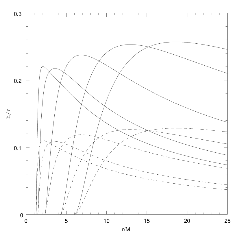
Figure 3: The ratio of the disk thickness to the radius. Shown are curves of $h(r)/r$ for $a/M=0$, $0.5$, $0.9$, $0.99$, and $0.998$. For each of these values of $a$ two curves are plotted: for $L=L_{edd}$ (solid lines) and $L=L_{edd}/2$ (dashed lines).

In Figure 3 we plot the ratio $h(r)/r$. The faster the black hole rotates the smaller the relative thickness of the disk becomes. As in Figure 3, the ratio $h/r$ is largest for a Schwarzschild black hole, reaching its maximum value of

$$\left(\frac{h}{r}\right)_{max}=0.257\left(\frac{L}{L_{edd}}\right)$$

at $r_{\ast}=18.62$.

One should notice that our assumption of isotropic turbulence made above is inconsistent with the thickness of the disk being constant in time. Because there is a component of turbulent velocity normal to the surface, the matter in the disk has to be in motion with a characteristic amplitude of $\simeq h$. Averaged over the characteristic time scale of turbulent flow, this effect leads to additional broadening of the line profile due to changes of the position of emitting spot. This broadening is correlated with Doppler turbulent broadening and, as a first approximation, can be included as a correction factor for the radial dependence of the quantity $c_{s}/c$ in equation (1). However, we lack knowledge about vertical structure of the disk and vertical motions, and we do not attempt to model the effects of temporal variations in $h(r)$. Instead we will consider only systematic redshifts connected with a time-averaged value of $h(r)$.

Finally, let us calculate the electron scattering optical depth $\tau_{es}$ along directions which are normal to the disk plane. It must be much larger than $1$ in order to produce a fluorescent iron line. The Novikov & Thorne model gives

$$\tau_{es}=1.84\varepsilon(a)\alpha^{-1}\left(\frac{L}{L_{edd}}\right)^{-1}r_{\ast}^{3/2}{\cal A}^{-2}{\cal B}^{3}{\cal C}^{1/2}{\cal E}{\cal Q}^{-1}\mbox{.}$$

Computations show that for the range of parameters of a thin disk model considered here, $0<a_{\ast}<0.998$, and $\alpha<0.3$, $L/L_{edd}<1$, the minimal value of $\tau_{es}(r_{\ast})$ is about $30$ and is achieved at $a=0.998$, $\alpha=0.3$, $L=L_{edd}$. Thus, the thin disk is always capable of producing an iron fluorescence line.

To summarize, in this section we have adopted the Novikov-Thorne disk model and used it to determine the relevant parameters for line emission in a turbulent disk. The key quantities are the sound speed and height of the disk. With these, we proceed to line profile calculations.

3 Imaging of an accretion Disk and Line Profiles Calculation

3.1 Ray tracing in a Kerr Metric

The standard Novikov-Thorne disk model provides us with all information necessary to calculate line profiles once we specify the emissivity function of the disk. We perform the calculation using a variant of the numerical ray-tracing code described by Bromley, Chen & Miller (1997). Briefly, the strategy is to generate a pixelized image of the accretion disk as would be seen by a distant observer. The observed frequency at each pixel is given by

$$g\equiv\frac{\nu_{o}}{\nu_{e}}=\frac{-1}{-\vec{u}\cdot\vec{p}}$$ (19)

where subscripts $o$ and $e$ are observer and emitter respectively, $\vec{u}$ is the 4-velocity of the emitter and $\vec{p}$ is the emitted photon’s 4-momentum. Note that the emitter 4-velocity is specified by the disk model, while the photon 4-momentum is calculated by numerically tracing the photon geodesic back in time from the pixel in the observer’s sky plane to the surface of the disk. The line profile then follows from making a histogram of the number of pixels versus frequency. Each frequency bin in the histogram is an accumulation of contributions from individual pixels, and thus represents an integral over the disk. The actual flux comes from weighting each bin by the local emissivity and $g^{4}$; three factors of $g$ come from the relativistic invariant $I_{\nu}/\nu^{3}$, where $I_{\nu}$ is the intensity, and the remaining factor arises because the line profile is an integrated flux. This weighting takes care of the effect of Doppler motions and gravitational redshifts. Note that Figure 3 of Bromley, Chen & Miller (1997) is incorrect, as the profile was generated with the $g^{3}$ weighting but is labelled as integrated flux. (The correct weight factor can be inferred from that paper; see the discussion surrounding eq. [7], therein.)

We do not take into account illumination of the disk by line photons emitted in other parts of the disk and possible reflection of those photons to the observer. Due to uncertainties in the illumination law and the fact that the flux in the line is still the small fraction of X-ray continuum at 4–10 keV, this is, probably, a justified approximation.

The ray tracer itself is a general-purpose second-order geodesic solver for a Kerr geometry. Our modification to this code enables an arbitrary axisymmetric disk surface to be specified so that the photon trajectories terminate (rather, originate) on this surface. The procedure is not entirely efficient, as our fourth-order Runge-Kutte integrator tends to overstep the surface. We could interpolate back from the overshoot, but we instead force smaller time steps and keep accuracy high. The loss of speed is not enormous. Even so, we put the problem to a parallel supercomputer and, when calculating line profiles, limit ourselves to images of 1024$\times$1024 pixels for high resolution.

While the prescription for calculating line profiles just given is complete, we comment incidentally on the calculation of the emitter 4-velocity, $\vec{u}$ in equation (19). Derivations of this quantity for thin ($h=0$) disks can be found in Bardeen, Press & Teukolsky (1972), Novikov & Thorne (1973) and Cunningham (1975). In our calculations we assume that outside of the orbit of marginal stability the bulk emitter 4-velocity is the sum of Keplerian 4-velocity and a small, inward radial velocity component as given by equation (16). We do not take into account the $\theta$ component of inflow velocity or the dependence of $\bar{v}^{\hat{r}}$ on the height of the disk. These are higher order corrections to radially directed inflow. Inside of the marginal stability radius, all orbits are presumed to be in freefall within the equatorial plane exactly (e.g., Cunningham 1975). As indicated in equation (1), we include the effects of turbulence by assuming a Gaussian turbulent spectrum in the local frame of the bulk flow of gas.

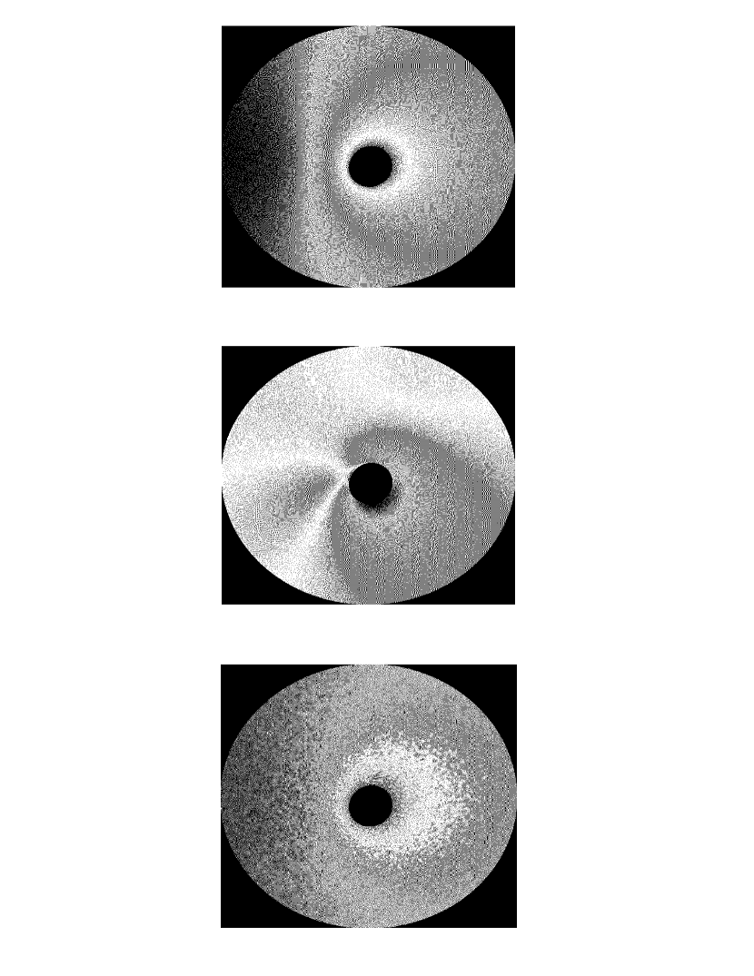
Figure 4: Artificial color redshift images of an accretion disk around a black hole (see text for explanations). Blue color indicates blueshift, red color indicates redshift. Figure (a) is at the top, figure (b) is in the middle and figure (c) is at the bottom of the plate. Full color figure in postscript format can be downloaded from http://pegasus.as.arizona.edu/~vpariev, file disk_image.ps

Example images of a disk around an extreme Kerr black hole with $a=0.998$ can be seen in Figures 4 (a), (b), and (c) (Plate 1). In these figures the inner and outer radii of the disk are placed at $1.237M$ (the innermost stable circular orbit) and $15M$, respectively, and the disk is viewed at $i=30^{0}$ with respect to polar axis. The false colors indicate the frequency shift of emitted photons as a result of Doppler and gravitational redshift. In order to demonstrate the effect of physical structure of the disk clearly we choose the values $\alpha=0.3$, $L/L_{edd}=1$ which are roughly upper limits allowed by the thin disk model. Figure 4(a) shows an image of an accretion disk with finite thickness considering only non-turbulent motion of the rotating gas slowly moving closer to the black hole. Finite thickness of the disk reveals itself in two ways: first, at a finite height above the equatorial plane, the gravitational field differs slightly from that in the equatorial plane of the black hole; second, the line-of-sight photon trajectory crosses the surface of the disk at a slightly different value of radial coordinate $r$ than if it crosses the equatorial plane, thus affecting the Keplerian circular velocity of the emitting gas. Both effects are comparable to each other and together with the Doppler shift from the radial inflow, they result in corrections to the value of redshift $g$ distributed over the disk surface in a quite complicated way.

Figure 4(b) is a false color map of the difference between redshift of pixels of images for the disk model shown in Figure 4(a) and redshifts for infinitesimally thin Keplerian disk. Analyzing this map one should take into account that the light bending effect causes the angle at which a light ray strikes the surface of the disk to be different from disk inclination angle $i$, especially in the inner regions of the disk. The frame dragging effect also causes asymmetry of the image of the inner edge of the disk (central black spot on images).

Finally, Figure 4(c) shows a redshift map of a turbulent disk including all effects of gas motion and thickness of the disk. Parameters of the disk are the same as in Figures 4(a) and (b), except that the turbulent velocity in the disk is assumed to have mean square equal to the sound speed. The effect of turbulence was accounted for by calculating $\sigma=c_{s}/\sqrt{3}$ and height $h(r)$ for each pixel. Then a random additional frequency shift was assigned to each pixel (Gaussian distributed, with zero mean and variance equal to $\sigma^{2}$) sampling the distribution of turbulent line broadening given by equation (1). In order to get a spatial coherence length of the turbulence $h(r)$ these random numbers were averaged for pixels within a radius $h(r)$. The variance of each averaged frequency shift ${\bar{x}}(r)$ is $\sigma^{2}/N$ where $N$ is the number of pixels inside radius $h(r)$. We actually want a random number that has a variance of $\sigma^{2}$, so we scale ${\bar{x}}(r)$ by a factor of $\sqrt{N}$. Compression of turbulent patches in the horizontal dimension — a result of rays intercepting the disk surface at more oblique angles — is clearly seen in the innermost part of the disk. Visual displacement of the central dark spot (“hole”) from the center of visual image of the disk is due to effects of finite disk thickness and gravitational bending of light.

3.2 Line Profiles

We now assess the effects of disk structure and turbulence on the line profiles. Using our binning algorithm we generated line profiles for different parameters of the disk–black hole system. We assumed that there is no emission coming from the region below innermost stable orbit $r_{ms}$ and the emissivity falls off with radius as a power law such that $\epsilon(r)\propto r^{-q}$. Fitting of observations suggests that $2<q<4$ (Tanaka et al. 1995; Iwasawa et al. 1996; Dabrowski et al. 1997) and the best studied object MCG-6-30-15 seems to have $q\approx 3$. We assume that the inner radius of the emitting part of the disk is $R_{in}=r_{ms}$, and for outer radius we assume $R_{out}=15M$ for $i=30^{0}$, $i=60^{0}$, and $R_{out}=20M$ for $i=75^{0}$. Examples of line profiles are shown in Figures 5 and 6 for $i=30^{0}$, $i=60^{0}$, and $i=75^{0}$ and square mean of $v_{tur}$ equal to $c_{s}$. Figures 7 and 8 show line profiles from the disk with the same parameters as in Figures 5 and 6, except that square mean of $v_{tur}$ is set to $\alpha c_{s}$. The major effects of gas motion in the disk are the broadening of the line profile, smoothing of the blue and red peaks and shift of the blue peak to the red. The former two effects are due to turbulent motions, while the latter one is due to the radial inflow velocity and additional redshift due to disk thickness. The shift of the blue peak toward the red increases with increasing luminosity and depends upon the illumination law, the value of the viscosity parameter $\alpha$, and the disk inclination angle. The maximum effect of finite disk thickness can be as large as about 10 percents.

In the case of ${\bar{v}}_{turb}=c_{s}$ the sharp blue edge of the line — which is very sensitive to the inclination angle — becomes smooth and more extended toward blue. On the other hand, the red tail of the line is not affected since it is formed close to inner edge of the disk where values of $c_{s}$, $v_{r}$ and $h$ becomes small in the Novikov–Thorne model. In the case of small values of turbulent velocity close to its lowest limit ${\bar{v}}_{turb}=\alpha c_{s}$, the sharp blue edge of the line also becomes smooth but its position remains almost unchanged. The reason is that the blueshift for a smaller value of $v_{tur}$ is balanced by the redshift because of the inflow velocity. The peak intensity of the line may be reduced by a factor of almost two because of the redistribution of flux to neighboring frequencies.

Another effect is the reduction of the total flux in the line with increasing the ratio of $L/L_{edd}$. This effect becomes larger with the increase of inclination angle and with the illumination more concentrated in the innermost parts of accretion disk (i.e., for larger $q$). For $a=0.998$, $i=75^{0}$, $q=4$, $L=L_{edd}$ the reduction in flux is almost three times compared to the thin disk case with the same emissivity law. When the disk gets thicker, light rays coming from an observer intersects surface of the disk at smaller angles, thus, making a solid angle of viewing the disk surface smaller and decreasing flux in the line. Changes in the angle of intersection are most pronounced for highly inclined disks and even shadowing of the inner parts of the disk by the outer parts can occur. Since gravitational bending of light increases closer to the black hole, rays which intersect the inner parts of the disk which lie nearest the observer are typically more oblique, and the point of intersection is typically at a larger radius. The result is an effective increase in the emissivity index $q$, and an overall reduction in the total flux in the line as compared to a thin disk with the same area in the observer’s sky plane. Thus, taking into account finite thickness of the disk reduces the equivalent width of the iron line by an amount strongly dependent upon the inclination angle of the disk and the emissivity index.

In summary, we see that proper treatment of kinematics and geometry of a disk with finite thickness can appreciably influence the shape of iron line profile if the accretion rate is such as $L\approx L_{edd}/2$ or higher.

4 Discussion and Conclusions

In the present work we extended previous calculations of iron line profiles from relativisitic accretion disks to include the effects of finite thickness, radial accretion flow and turbulence. We adopt the Novikov-Thorne solution for a thin disk model with Gaussian distribution of turbulent velocities with variance equal to the local speed of sound, and find with fully relativistic, numerical ray-tracing calculations that turbulent broadening is generally the dominant effect. The most prominent changes in the skewed, double-horned line profiles are a substantial reduction in the maximum flux at both red and blue peaks, a redistribution of radiation into the wings and a tendency for the blue peak to shift toward the red. These effects are most pronounced when inner disk radii are most emissive, the inclination angles are large, turbulence motions approach the sound speed, and the accretion rate is high.

Turbulent broadening of a line profile depends linearly on the ratio of the luminosity of the disk to Eddington limit, which is the crucial parameter controlling the magnitude of the effect. For $L/L_{edd}=1$ the effect is generally about 10% and is, thus, of the order of the signal–to–noise for best measured line profiles. Since we do not know the ratio $L/L_{edd}$ for most AGN — the black hole masses are not well-constrained — we cannot estimate how important turbulent broadening is for the observed objects considered here.

We also found that finite thickness of the disk causes a reduction in the total intensity of the line profile, since the surface of the innermost part of a thick disk is viewed at a smaller angle, resulting in a decrease of the solid angle spanned by the disk on the sky. This reduction of the iron line equivalent width strongly increases with inclination angle of the disk, accretion rate, and emissivity index $q$.

We have considered only kinematics and geometry of a turbulent disk, leaving more detailed treatment of iron line formation processes for future work. Of these processes, changes in the rest-frame energy of the line as a result of varying ionization are among the most important. The effect of appearance 6.97-keV line of Fe 26 together with 6.4-keV line is at the same 10% level as the effect of turbulent Doppler shift. Thermal broadening of the line may be important as well in high quality data from future X–ray missions. Another physical effect which we did not take into consideration and which can have a significant influence on the observed line profile and equivalent width of iron line is Compton scattering of the radiation by hot (possibly nonthermal) electrons in an extended corona of the disk. This effect can cause angular dependence of the line and anisotropy of its emission. Such calculations are also very model-dependent but may result in correlation of the width of the iron line with the X-ray luminosity of the galaxy and spectral characteristic of continuous X-ray emission. Nonetheless, the consideration of disk kinematics and geometry is an important step toward obtaining a more complete picture of the central engines in active galaxies.

Figure 1: The dependencies $v_{tur}=c_{s}(r/M)$ (dashed lines), $\bar{v}^{\hat{r}}(r/M)$ (solid lines), and $\hat{v}_{T}(r/M)$ (dashed–dotted line). Each of these quantities is plotted for five values of rotational parameter $a/M=0$, $0.5$, $0.9$, $0.99$, and $0.998$. The value of $a$ increasing, the inner disk radius, at which both sound speed and radial inflow velocity are $0$, decreases. $M=10^{8}M_{\odot}$, plots are for two different values of each $L/L_{edd}$ and $\alpha$.

Figure 2: Same as in Fig. 1 but dashed lines are for the dependencies of $v_{tur}=\alpha c_{s}(r/M)$.

Figure 5: The integrated flux $F$ as a function of observed frequency $\nu$ (in units of the emitted frequency $\nu_{e}$) for accretion disk in Schwarzschild system at three different inclination angles $i=30^{0}$, $60^{0}$, and $75^{0}$ and three values of emissivity index $q=2$, $3$, and $4$ (figures a, b and c). The inner radius of the emissive part of the disk is $6\,M$. The outer radius of the emissive part of the disk is $15\,M$ for $i=30^{0}$, $60^{0}$ and $20\,M$ for $i=75^{0}$. Mean square of turbulent velocity is $c_{s}$. On each plot line profiles for three different values of disk luminosity are shown. Line profiles from infinitesimally thin Keplerian disk are shown in solid. Dotted line profiles are for turbulent disk with $L=L_{edd}/2$ and $\alpha=0.3$, dashed line profiles are for turbulent disk with $L=L_{edd}$, $\alpha=0.3$.

Figure 6: The integrated flux $F$ as a function of observed frequency $\nu$ (in units of the emitted frequency $\nu_{e}$) for accretion disk in extreme Kerr system. Inner radius of the disk is at $r=r_{ms}=1.237\,M$. Outer radius of the disk is $15\,M$ for $i=30^{0}$, $60^{0}$ and $20\,M$ for $i=75^{0}$. Line profiles from infinitesimally thin Keplerian disk are shown in solid. Dotted lined profiles are for turbulent disk with $L=L_{edd}/2$ and $\alpha=0.3$, dashed line profiles are for turbulent disk with $L=L_{edd}$, $\alpha=0.3$. Other parameters are similar to those in Fig. 5.

Figure 7: Same as in Fig. 5 except that the mean square of turbulent velocity is $\alpha c_{s}$ here.

Figure 8: Same as in Fig. 6 except that the mean square of turbulent velocity is $\alpha c_{s}$ here.

- (1) Abramowicz, M.A., Lanza, A., & Percival M.J. 1997, ApJ, 479, 179
- (2) Bardeen, J.M., & Peterson, J.A. 1975, ApJ, 195, L65
- bard (2) Bardeen, J.M., Press, W.H., & Teukolsky, S.A. 1972, ApJ, 178, 347
- (4) Bromley, B.C., Chen, K., & Miller, W.A. 1997, ApJ, 475, 57
- (5) Bromley, B.C., Miller, W.A., & Pariev, V.I. 1998, Nature, 391, 54
- (6) Chen, K., & Halpern, J.P. 1989, ApJ, 344, 115
- (7) Cunningham, C.T. 1975, ApJ, 202, 788
- (8) Dabrowski, Y., Fabian, A.C., Iwasawa, K., Lasenby, A.N., & Reynolds, C.S. 1997, MNRAS, 288, L11
- (9) Dörrer, T., Riffert, H., Staubert, R., & Ruder, H. 1996, A&A, 311, 69
- (10) George, I.M., & Fabian, A.C. 1991, MNRAS, 249, 352
- (11) Fabian, A.C., Rees, M.J., Stellar, L., & White, N.E. 1989, MNRAS, 238, 729
- (12) Iwasawa, K., Fabian, A.C., Reynolds, C.S., Nandra, K., Otani, C., Inoue, H., Hayashida, K., Brandt, W.N., Dotani, T, Kunieda, H., Matsuoka, M. & Tanaka, Y. 1996, MNRAS, 282, 1038
- (13) Laor, A. 1991, ApJ, 376, 90
- (14) Matt, G., Fabian, A.C., & Ross, R.R. 1996, MNRAS, 278, 1111
- matt (2) Matt, G., Fabian, A.C., & Ross, R.R. 1993, MNRAS, 262, 179
- matt (3) Matt, G., Perola, G.C., & Piro L. 1991, A&A, 247, 25
- matt (4) Mushotzky, R.F., Fabian, A.C., Iwasawa, K., Kunieda, H., Matsuoka, M., Nandra, K., & Tanaka, Y. 1995, MNRAS, 272, L9
- (18) Nandra, K., George, I.M., Mushotzky, R.F., Turner, T.J., & Yaqoob, T., 1997, ApJ, 477, 602
- (19) Novikov I.D., & Thorne K.S. 1973, in Black Holes, eds. DeWitt C., DeWitt B.S. (New York:Gordon and Breach), 343
- (20) Page, D.N., & Thorne, K.S. 1974, ApJ, 191, 499
- (21) Peitz, J., & Appl, S. 1997, MNRAS, 286, 681
- (22) Reynolds, C.S., & Begelman, M.C. 1997, ApJ, 488, 109
- (23) Reynolds, C.S., & Fabian, A.C. 1997, MNRAS, 290, L1
- (24) Riffert, H., & Herold, H., 1995, ApJ, 450,508
- (25) Ross, R.R., & Fabian, A.C., 1993, MNRAS, 261, 74
- (26) Rybicki, G.B., & Bromley, B.C., 1998, ApJ, submitted
- (27) Tanaka, Y., Nandra, K., Fabian, A.C., Inoue, H., Otani, C., Dotani, T., Hayashida, K., Iwasawa, K., Kii, T., Kunieda, H., Makino, F., & Matsuoka, M. 1995, Nature, 375, 659
- (28) Thorne, K.S., 1974, ApJ, 191, 507
- (29) Życki, P.T., & Czerny, B. 1994, MNRAS, 266, 653