Gravitational Magnification of Pop III Supernovae in
Hierarchical Cosmological Models: NGST Perspectives

Abstract

We study the gravitational lensing magnification produced by the intervening cosmological matter distribution, as deduced from three different hierarchical models (SCDM, LCDM, CHDM) on very high redshift sources, particularly supernovae in protogalactic (Pop III) objects. By means of ray-shooting numerical simulations we find that caustics are more intense and concentrated in SCDM models. The magnification probability function presents a moderate degree of evolution up to $z\approx 5$ (CHDM) and $z\approx 7$ (SCDM/LCDM). All models predict that statistically large magnifications, $\mu\lower 2.15277pt\hbox{$\;\buildrel>\over{\sim}\;$}20$ are achievable, with a probability of the order of a fraction of percent, the SCDM model being the most efficient magnifier. All cosmologies predict that above $z\approx 4$ there is a 10% chance to get magnifications larger than 3. We have explored the observational perspectives for Pop III SNe detection with NGST when gravitational magnification is taken into account. We find that NGST should be able to detect and confirm spectroscopically Type II SNe up to a redshift of $z\approx 4$ in the J band (for $T_{SN}=25000$ K); this limit could be increased up to $z\approx 9$ in the K band, allowing for a relatively moderate magnification. Possibly promising strategies to discriminate among cosmological models using their GL magnification predictions and very high-$z$ SNe are sketched. Finally, we outline and discuss the limitations of our study.

1 Introduction

Current models of cosmic structure formation based on CDM scenarios predict that the first collapsed, luminous (hereafter Pop III) objects should form at redshift $z\approx 30$ and have a total mass $M\approx 10^{6}M_{\odot}$ or baryonic mass $M_{b}\approx 10^{5}M_{\odot}$ (Couchman & Rees 1986, Ciardi & Ferrara 1997, Haiman et al. 1997, Tegmark et al. 1997, Ferrara 1998). This conclusion is reached by requiring that the cooling time, $t_{c}$, of the gas is shorter than the Hubble time, $t_{H}$, at the formation epoch. In a plasma of primordial composition the only efficient coolant in the temperature range $T\leq 10^{4}$ K, the typical virial temperature of Pop III dark matter halos, is represented by H₂ molecules whose abundance increases from its initial post-recombination relic value to higher values during the halo collapse phase.

Thus, as the collapse proceeds, the gas density increases and stars are likely to be formed. However, the final product of such star formation activity is presently quite unknown. This uncertainty largely depends on our persisting ignorance on the fragmentation process and its relationship with the thermodynamical conditions of the gas, both at high $z$ and, in a less severe manner, in present day galaxies. Ultimately, this prevents firm conclusions on the mass spectrum of the formed stars or their IMF. This problem was already clear more than two decades ago, as pioneering works (Silk 1977; Kashlinsky & Rees 1983; Palla, Salpeter & Stahler 1983; Carr et al. 1984) could not reach similar conclusions on the typical mass range of newly formed stars in the first protogalactic objects. Roughly speaking, two possibilities can be envisaged: either (i) a limited number of Very Massive Objects (VMOs), single stars with mass in the range $10^{2}-10^{5}M_{\odot}$ could be formed, or (ii) a more common stellar cluster, slightly biased towards low-mass stars (or, even, some combination of the two involving low-mass star coalescence to form a VMO). Apart from the fact that observational evidences of the VMO hypothesis are still lacking in the local universe, there are also several theoretical problems (El Eid et al. 1983; Ober et al. 1983) that make VMOs as unlikely stellar prototype candidates in the early universe. Then, if the IMF is more of the standard type, questions arise about its shape and median value. A common claim in the literature is that the absence of metals (as it is the case in a collapsing Pop III) should shift the peak and the median of the IMF toward higher masses. Obviously, assessing the presence of massive stars that produce ionizing photons and die as Type II supernovae (SNe) would be of primary importance to clarify the role of Pop IIIs in the reionization and rehating of the universe, and, in general, for galaxy formation. Thus, studying the formation of the first stars has become one of the most challenging problems in physical cosmology. It is not the aim of this paper to investigate this aspect further; detailed studies can be found in Gnedin & Ostriker 1997, Haiman & Loeb 1997, and Ciardi & Ferrara 1997. Here, we simply point out that if SNe are allowed to occur at these very high redshifts, they could outshine their host protogalaxy by orders of magnitude and likely become the most distant observable sources since the QSO redshift distribution has an apparent cutoff beyond $z\approx 4$. Nevertheless, even for (future) large telescopes as NGST, VLT and Keck this will not be an easy task, this requiring to reach limiting magnitudes $\approx 33$ in the near IR to observe a SN exploding at $z=10$. Fortunately, the matter distribution in the universe behaves like a gravitational lens that distorces, and, most importantly here, magnifies the source flux. This magnification, as we will see, strongly enhances the detection probability of Pop III SNe, bringing their apparent magnitudes inside the instrumental capability range. A different, but complementary, strategy would be to monitor the central regions of nearby galaxy clusters (Miralda-Escudé & Rees 1997), where magnifications high enough to allow for the detection of faint objects could be produced. We have chosen to investigate the gravitational lensing (GL) magnification effects of the entire cosmological mass distribution to verify if the different GL magnification predictions of the most attractive cosmological models could be used as a test bench of their descriptive power of the universe. Pushing this comparison to high redshift, as we will see, is crucial since magnification properties deduced from hierarchical models start to differentiate considerably only beyond $z\approx 5$.

Gravitational lensing is sensitive to the cosmic mass distribution, which in turn depends on the adopted fluctuation spectrum, to the expansion factor, and to cosmological distances; therefore, it represents a perfect tool for cosmological studies. As stated above, our aim is to calculate GL effects on high $z$ sources, as for example SNe in Pop III objects, and, in particular, the magnification probability as a function of the source redshift and of the cosmological model. In order to obtain this result it is necessary to define how structure is formed in the universe and a method to evaluate the statistical incidence of GL effects. The former problem may be approached by the linear perturbation theory of cosmic density fluctuations, numerical N-body simulations or by semi-analytical methods, as, for example, the Press & Schechter (1974, hereafter PS) formalism. GL can be investigated both by numerical simulations following light propagation or via semi-analytical estimates. We have chosen to solve the selected problem by using simulations based on the so-called ray-shooting numerical scheme as far as GL is concerned and to derive the mass and redshift distribution of the lens ensamble from PS. The reasons for this choice are motivated below (see § 2); in general, we find that the ray-shooting + PS approach constitutes a flexible and accurate enough tool for our purposes. The PS approach has been used also in conjuction with analytical techniques by several authors (Narayan & White 1988, Kochanek 1995, Nakamura & Suto 1997).

This approach is somewhat different with respect to others used in past literature to investigate analogous problems. Schneider & Weiss (1988) have applied the ray-shooting scheme to study the propagation of light in a clumpy universe and to derive information on the influence of matter inhomogeneities on the apparent luminosity of lensed sources. The main difference with that work, is that we allow the lens mass to be distributed according to the prescriptions of a given cosmological model, rather than assuming identical clumps of mass $M$. Essentially for the same reasons, our work differs also from the one presented by Lee & Paczynski (1990), who consider GL in a flat spacetime and approximate the true three-dimensional distribution of matter with multiple identical screens. Jaroszyński (1991) allows for density fluctuation to grow starting from the particular initial power spectrum $\propto k^{-3}$ (which is at the limit of the hierarchical structure formation model) and superimposing a galaxy population whose mass distribution is inferred from the Schechter function and a prescription for the $M/L$ ratio. The delicate assumption that galaxies trace mass in the universe, as well as the use of the Schechter distribution at high redshift, appears difficult to be justified, however.

Massive computational methods coupling the full power of N-body simulations and ray-shooting start to become available in the literature (Wambsganss et al. 1996; Premadi et al. 1997), although with some unavoidable limitations which make them suitable for more focussed studies. Wambsganss et al. (1996) examined the evolution of various GL statistical indicators (i.e. multiple image frequency, lens redshift distribution, magnification maps, caustic and critical line geometry) in a CDM model up to $z=3$. In the second work, gravitational shear and magnification of a single light beam produced by lenses in the redshift range $z=0-5$ for three cosmological models are calculated. Our work is intended to mainly explore the magnification effects produced by the cosmological matter distribution deduced from three different hierarchical models (SCDM, LCDM, CHDM whose parameters are given in § 2) on very high redshift sources. Particular emphasis is devoted to the perspectives offered by GL for the observational detection of SNe in protogalactic objects. We also explain how such observations could help constrain the validity of the proposed classes of cosmological models.

The plan of the paper is as follows. In the next Section we define the cosmological models under study and derive their predicted lens mass distribution; in § 3 we introduce and discuss the basic concepts of thick gravitational lenses. Sec. 4 is devoted to the description of the numerical scheme used for the GL simulations whose results are presented in § 5. Sec. 6 contains the observational implications of our results for future detection of high-$z$ SNe with NGST; finally, the discussion and summary in § 7 conclude the paper.

2 Cosmological Lens Distribution

As stated above, our main aim is to determine the GL effects due to the intervening cosmological mass distribution on distant sources. Currently, the most attractive models for structure formation in the universe, assume that perturbations grow from an initial gaussian field of fluctuations with a scale-free power spectrum. These perturbations become nonlinear at redshift $\approx 50$ and form bound objects, which subsequently merge to form larger and larger structures in a hierarchical fashion. In spite of the relatively widespread agreement on this general scenario, a detailed comparison of the predictions of such type of models with observational data does not allow yet to discriminate among the various hierarchical models so far proposed and to uniquely fix their free parameters.

Given these uncertainties, and with the hope to constrain at least some of the properties of the proposed models, we will consider and compare three different cosmological models with the same total density parameter $\Omega=\Omega_{M}+\Omega_{\Lambda}+\Omega_{\nu}=1$, contributed by cold dark matter + baryons, cosmological constant $\Lambda$, and hot dark matter, respectively. In particular, (i) Standard Cold Dark Matter (SCDM), has $\Omega_{M}=1,\Omega_{\Lambda}=\Omega_{\nu}=0$; (ii) Lambda Cold Dark Matter (LCDM) has $\Omega_{M}=0.4,\Omega_{\Lambda}=0.6,\Omega_{\nu}=0$; finally, (iii) Cold+Hot Dark Matter (CHDM) parameters are $\Omega_{M}=0.7,\Omega_{\Lambda}=0,\Omega_{\nu}=0.3$.

In order to specify the spectrum completely we have to fix both the present value of the Hubble constant $H_{0}=100h$ km s^-1 Mpc^-1, and the normalization of the spectrum, often parameterized by its gaussian variance (see eq. 2 below) $\sigma_{8}=\sigma(8h^{-1}$ Mpc). The value of $h$ remains uncertain by about a factor of two: $0.4\leq h\leq 1$. Standard relative distance methods using Type Ia SNe (Garnavich et al. 1997, Perlmutter et al. 1998, Kim et al. 1997) tend to favor higher values of $h\approx 0.6-0.8$, whereas methods based on fundamental physics methods, including GL, suggest lower values $h\approx 0.4-0.6$ (Grogin & Narayan 1996; Kneib 1998 and references therein). For this reason, we adopt the intermediate value $h=0.65$ throughout the paper; fixing $h$ has the advantage that, when comparing the predictions of the various models, one can isolate differences that depend only on their intrisic properties listed above. The second point concerns the normalization of the power spectrum. The actual form of the power spectrum can be obtained by numerically integrating the relevant numerical equations; we use the analytical fit to such results provided by Efstathiou et al. (1992):

$$|\delta_{k}|^{2}=\frac{\displaystyle Ak^{n}}{\displaystyle\left\{1+\left[Bk+(Ck)^{3/2}+(Dk)^{2}\right]^{\nu}\right\}^{2/\nu}},$$ (1)

where $\nu$=1.13; $B$=6.4 $h\Gamma$ Mpc; $C$=3.0 $h\Gamma$ Mpc; $D$=1.7 $h\Gamma$ Mpc, $n$=1; $\Gamma$ is the shape parameter and it is equal to $\Gamma=h$ for SCDM, $\Gamma=h\Omega_{M}$ for LCDM, $\Gamma=0.2(0.3/\Omega_{\nu})^{1/2}$ for CHDM. The coefficient $A$, or equivalently the value of $\sigma_{8}$, must be determined by choosing an appropriate normalization. We fix $\sigma_{8}$ such that the number of clusters present at $z=0$, about one per $(100h^{-1}Mpc)^{3}$, is correctly reproduced. This implies $\sigma_{8}=0.64,1.07,0.68$, for SCDM, LCDM, CHDM, respectively.

Once the spectrum has been fully specified, the structure formation and evolution can be determined, for example, via N-body numerical simulations. Here we take a complementary approach that makes use of the Press-Schechter (PS) formalism (Press & Schechter 1974; Bardeen et al. 1986; Peacock & Heavens 1990; Bond et al. 1991) in its standard form; we will briefly discuss later in this Section the main advantages and limitations of such approach. Given a power spectrum $|\delta_{k}|^{2}$ (in our case eq. 1) one can write the gaussian variance of the fluctuations on the mass scale $M$:

$$\sigma_{M}^{2}=\int\frac{d^{3}k}{(2\pi)^{3}}W^{2}(k,R)|\delta_{k}|^{2},$$ (2)

where $M=(4/3)\pi\rho R^{3}$, $\rho$ is the matter density, and

$$W={3\over(kR)^{3}}\left[\sin(kR)-(kR)\cos(kR)\right];$$ (3)

is a top-hat filter function. From the results of the nonlinear theory of gravitational collapse, stating that a spherical perturbation with overdensity $\delta_{c}=\delta\rho/\rho>1.69$ with respect to the background matter collapses to form a bound object, through the PS formalism we can derive the normalized fraction of collapsed objects per unit mass at a given redshift:

$$f(M,z)=\sqrt{\frac{2}{\pi}}\frac{\delta_{c}(1+z)}{\sigma_{M}^{2}}e^{-\delta_{c}^{2}(1+z)^{2}/2\sigma_{M}^{2}}\left(-\frac{d\sigma_{M}}{dM}\right).$$ (4)

A useful quantity is the cumulative mass function

$$F(M,z)=\int^{M}_{0}f(M,z)dM={\it erf}\left(\frac{\delta_{c}(1+z)}{\sqrt{2}\sigma_{M}}\right).$$ (5)

In Fig. 1, as an example, we show the function $f(M,z)M$, which gives the fraction of collapsed objects per unit logarithmic mass for the three cosmological models and two different redshifts.

The PS formalism has been shown to be in surprisingly good agreement with the results from N-body numerical simulations (Brainerd & Villumsen 1992, Gelb & Bertschinger 1994, Lacey & Cole 1994, Klypin et al. 1995). Nevertheless, it suffers from several limitations (for a discussion see, for example, Yano et al. 1996; Porciani et al. 1996), and that the complexity of structures in the universe cannot be described in full detail. There are at least two pieces of information that are not present in the PS recipe: (i) the internal structure, i.e. the density profile, of the collapsed objects, and (ii) their spatial distribution at a given redshift. In general, these aspects are relevant in GL experiments and for this reason, as we will discuss in the next Section, one has to make some additional hypothesis. Since we approach the study of GL effects using statistical methods, the bias introduced by those assumptions needs to be evaluated carefully; we leave this to the final Section. However, obtaining the mass distribution as a function of redshift with PS, not mentioning its widespread use in literature and in GL studies that allows for straight comparisons and checks, has the advantage that it is computationally convenient and therefore the parameter space exploration and the optimization of the GL numerical scheme (see §4) can be performed with relatively unexpensive procedures. For these reasons we feel that is worthwhile to attack the problem with these approximate techniques that can represent a useful complement to more massive future computations.

3 Thick Gravitational Lenses

In this paper, we are interested in determining the GL magnification properties of high redshift sources (typically SNe) due to the intervening cosmological matter distribution. Since this matter distribution, as obtained from N-body simulations and/or PS formalism, covers a large range of redshifts, the standard assumption that the lensing mass is concentrated on a single plane perpendicular to the propagation of the reference light ray (i.e. the optical axis) has to be modified to include such spread. This can be achieved by splitting the mass distribution on a series of planes, and furthermore postulating that (i) deflections on the various planes are independent and (ii) the trajectory of a light ray is modified only at planes. These deflections can be calculated through the deflection potential $\Psi_{z}(\xi_{z})$, where $z$ refers to the redshift of the plane and $\xi_{z}$ is the impact parameter on that plane; the propagation between planes can be generally described by the Dyer-Roeder (1972) equation, also discussed by Futamase & Sasaki (1989), Babul & Lee (1991), and Nakamura (1997). In brief, the main requirement when using Dyer-Roeder distances is that the redshift intervals are $\lower 2.15277pt\hbox{$\;\buildrel<\over{\sim}\;$}1$, in order to fulfill the underlying hypotheses of the theory, i.e. a light ray bundle is not affected by nonlocal gravitational effects (shear) and significative local deflections. The validity of the above scheme, which pundits call a ”Thick Gravitational Lens”, is discussed in detail by Seitz et al. (1994), Seitz & Schneider (1994), but also in Schneider et al. (1992) and Schneider (1997). In the following we describe how we model the lens systems corresponding to the various cosmological models using the above approximation.

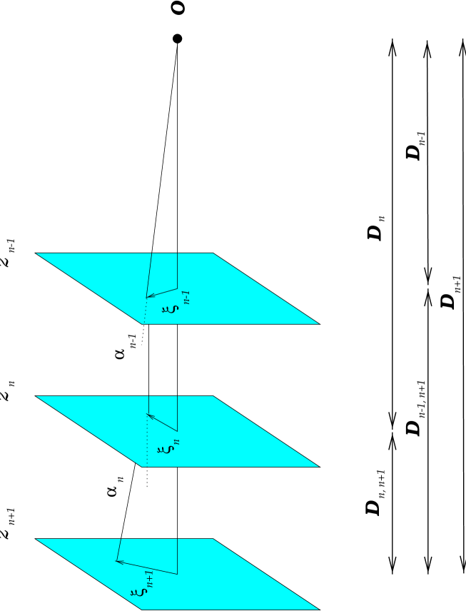
Figure 2: Schematic view of the Thick Gravitational Lens scheme with symbols defined in the text.

Let us suppose to split the mass on $N$ planes, at redshift $z_{1},z_{2},..,z_{n},..,z_{N}$, equally spaced with redshift interval $\Delta z<1$ both for the above reasons related to the use of Dyer-Roeder equation, and to correctly sample the cosmic mass distribution eq. 4. A sketch of such configuration is given in Fig. 2. Then the impact parameter on the plane $n+1$ is given by

$$\xi_{n+1}=-\frac{(1+z_{n-1})D_{n,n+1}}{(1+z_{n})D_{n-1,n}}\xi_{n-1}+\frac{D_{n-1,n+1}}{D_{n-1,n}}\xi_{n}-D_{n,n+1}\nabla_{\xi}\Psi_{z_{n}}(\xi_{n}),$$ (6)

where the deflection potential is

$$\Psi_{z}(\xi_{z})={4G\over c^{2}}\int d^{2}\xi^{\prime}\Sigma_{z}(\xi^{\prime})\ln\left(\frac{|\xi_{z}-\xi^{\prime}|}{\xi_{0}}\right);$$ (7)

$\Sigma_{z}$ is the mass surface density on the plane at redshift $z$ and $\xi_{0}$ is an arbitrary length scale. The angular distance $D_{ij}=D(z_{i},z_{j})$ is determined by solving the Dyer-Roeder equation in the form suggested by Linder (1988a, 1988b)

$$\ddot{D}+\frac{3+q(z)}{1+z}\dot{D}+\frac{3}{2}(1+z)^{-2}D\sum_{s}(1+s){\cal A}_{s}(z)\Omega_{s}(z)=0.$$ (8)

Here the dot indicates redshift derivatives; $s$ is defined by the equation of state $p=\Sigma_{s}s\rho_{s}$ involving the total pressure and the various density contributions, including the cosmological constant, in a Friedmann-like universe; for example, $s=-1$ for the cosmological constant, whereas $s=0$ for a dust universe. Finally, a convenient expression for the generalized deceleration parameter $q(z)$ is (Linder 1988a)

$$q(z)=-\frac{a\ddot{a}}{\dot{a}^{2}}=\frac{\sum_{s}\Omega_{s}(1+3s)(1+z)^{1+3s}}{\sum_{s}\Omega_{s}(1+z)^{1+3s}};$$ (9)

${\cal A}_{s}$ is the so-called Dyer-Roeder parameter that expresses the degree of homogeneity of the universe, i.e. ${\cal A}_{s}=1$ corresponds to a perfectly homogeneous matter distribution, ${\cal A}_{s}=0$ corresponds to the case in which all the matter is in bound systems. In general, eq. 8 can be solved only numerically once the appropriate boundary conditions are specified; in a few limiting cases, though, analytical solutions can be found. For the case of interest here, in which the matter is supposed to be clumped in a discrete number of collapsed objects projected onto the various planes, the relevant limiting case is ${\cal A}_{s}=0$ for which the following solution holds:

$$D(z_{1},z_{2})=(1+z_{1})[D(z_{2})-D(z_{1})],$$ (10)

where

$$D(z)={c\over H_{0}}\int_{1}^{1+z}\frac{dy}{y^{3}\sqrt{\sum_{s}\Omega_{s}y^{1+3s}}}.$$ (11)

This is the formula we use to calculate distances in eq.6. We note that the relation between the Dyer-Roeder angular distance and the more familiar luminosity distance, $D_{L}$ is always equal to $D=(1+z)^{-2}D_{L}$.

The deflection angle caused by the n-th plane, $\alpha_{z_{n}}(\xi_{n})$ is defined as the gradient of the deflection potential entering eq. 6. Throughout this paper we will assume for simplicity and for computational economy that lenses are point-like masses, an approximation whose limitations are discussed in § 7. The mass distribution of this lens ensamble is derived via the PS formalism (eq. 4). It is easy to verify that in this case

$$\alpha_{z_{n}}(\xi_{n})=\nabla_{\xi}\Psi_{z_{n}}(\xi_{n})=\frac{4GM_{*}}{c^{2}}\sum_{j}\frac{M_{j}^{(n)}}{M_{*}}\frac{\xi_{n}-\xi_{j}^{(n)}}{|\xi_{n}-\xi_{j}^{(n)}|^{2}},$$ (12)

where $M_{*}$ is a reference mass and $j$ runs on all the objects on the n-th plane; $\xi_{j}^{(n)}$ is the position of the j-th mass on the n-th plane, $M_{j}^{(n)}$. In GL studies it is very common to use angular coordinates rather than linear ones in order to define the deflection of light rays. We follow this tradition by introducing the angular impact parameter $\theta_{n}=\xi_{n}/D_{n}$, where $D_{n}$ is the distance from the observer to the $n$-th plane. Eq. 6 then becomes (also using eq. 12)

$$\theta_{n+1}=\frac{I_{n-1}^{n+1}}{I_{n-1}^{n}}\theta_{n}-\frac{I_{n}^{n+1}}{I_{n-1}^{n}}\theta_{n-1}-(1+z_{n})I_{n}^{n+1}\frac{4GM_{*}H_{0}}{c^{3}}\sum_{j}\frac{M_{j}^{(n)}}{M_{*}}\frac{\theta_{n}-\theta_{j}^{(n)}}{|\theta_{n}-\theta_{j}^{(n)}|^{2}},$$ (13)

where the auxiliary variable $I_{i}^{j}=(c/H_{0})(D_{i}^{-1}-D_{j}^{-1})$ has been used. From eq. 13 one can appreciate the existence of a characteristic redshift-independent value of $\theta$ which will be used as the natural unit angle for the numerical simulations

$$\theta_{u}=\sqrt{\frac{4GM_{*}H_{0}}{c^{3}}}\simeq 2\times 10^{-6}\sqrt{\frac{M_{*}}{M_{\odot}}}{\rm arcsec}.$$ (14)

Because of image splitting and distortion, GL produces a magnification of the flux from a given source. This can be understood by recalling that the angular size of the source is increased and, since the surface brightness is conserved, the net flux received is olso increased. In principle, we can calculate the total magnification $\mu$ (i.e. including all the possible multiple images) of a source located, for example, on the plane $\theta_{N}$ iteratively by using eq. 13:

$$\mu^{-1}(\theta_{1})=\det\left|\left|{\partial\theta_{N}\over\partial\theta_{1}}\right|\right|$$ (15)

and summing over all multiple images. Regions in the source plane for which $\mu\to\infty$ are known as caustics. In practice, this method can be applied only to a very limited number of cases in which the lens equation can be inverted, that is $\theta_{1}$ can be expressed as a function of $\theta_{N}$. In the next Section we will describe how $\mu$ is calculated in practice within the numerical scheme used to solve the problem.

4 Numerical Simulations: Method and Description

The problem in which we are interested here, i.e. the magnification of distant sources by the intervening cosmological distribution, and outlined in the previous Sections, cannot be solved by any analytical technique. Thus, we have to resort to numerical simulations; in particular we adopt the so-called ray-shooting method. A full description of this scheme can be found, for example, in Wambsganss (1990) (see also Schneider & Weiss 1988); in the following we outline only its main features.

Let us consider a given cosmic solid angle, $\omega$, and study the propagation of light rays through it; the main idea of ray-shooting is to follow such propagation in a direction that is opposite to the physical one, namely from the observer to the source. This propagation from a plane to the next one is mapped by eq. 13 above for each ray. Thus, illuminating all the images produced by the mass distribution contained in $\omega$, we can obtain an accurate description of the spatial pattern of the caustics and calculate the source magnification.

We now determine the cosmological mass distribution to be projected onto the various planes. We start by calculating the total mass contained in the cone defined by the solid angle $\omega$. The comoving volume of such cone between the two redshifts $z_{1}$ and $z_{2}$ is given by (Linder, 1988a; Carrol et al. 1992)

$$V(\omega,z_{1},z_{2})=\omega(\frac{c}{H_{0}})^{3}\int_{z_{1}}^{z_{2}}dz\frac{H_{0}}{H(z)}\left[\int_{1}^{1+z}\frac{dy}{y\sqrt{\sum_{s}\Omega_{s}y^{1+3s}}}\right]^{2},$$ (16)

where $H(z)$ is the Hubble constant at redshift $z$. The corresponding total mass is then simply ${\cal M}_{1,2}=(\Omega_{M}+\Omega_{\nu})\rho_{c}V(\omega,z_{1},z_{2})$, where the critical density $\rho_{c}=(3H_{0}^{2}/8\pi G)$. We then subdivide this mass among various point lenses distributed according to the prescribed mass distribution function obtained from PS (eq. 5) and appropriate for the cosmological model (SCDM, LCDM, CHDM) under study. Specifically, we extract via a Monte Carlo procedure values of the masses from such distribution, until their sum exceeds the value of ${\cal M}_{i,j}$ calculated for the two redshifts bracketing the redshift of the relevant plane. This coupled PS+Monte Carlo procedure, being very flexible and handy, can be used to extract from any hierarchical cosmological model the information required for the setup of a GL numerical experiment. Since the PS formalism does not provide us with any information about the spatial distribution of the collapsed structures (we neglect in this paper any GL effect related to the possible different distribution of baryons), it is necessary to make an ad hoc hypothesis concerning it. The simplest assumption is that the lenses are spatially uncorrelated and randomly distributed on the planes. Of course, this neglects the fact that in reality a certain, albeit not completely understood, degree of clustering could be present even at very high redshift. The limitation of this and the point lens hypotheses, that are the main ones in this paper, will be further discussed in §7.

With this background, we are now ready to describe the main features of the numerical computations and of the determination of the magnification probability of a lensed source. On the first plane, we define an orthogonal grid made of $N_{l}\times N_{l}$ pixels of size $\Delta_{l}$ and we shoot a light ray at each cell center. We then apply the lens equation 13 to the angular impact position $\theta_{1}$ of each ray to obtain all the subsequent positons $\theta_{2},\theta_{n},\theta_{N}$ up to the source plane. There we collect the final impact position in another grid made of $N_{s}\times N_{s}$ cells of size $\Delta_{s}$. The choice of $\Delta_{s}$ must be a compromise to minimize the effects of two statistical biases: on the one hand the number of rays collected in each cell has to be large enough to allow for a good statistical significance of averages; on the other hand, cells that are too large to prevent good spatial resolution of the caustic patterns. For this reason we constrain $\Delta_{s}$ to be

$$\Delta_{l}\ll\Delta_{s}\ll L_{s},$$ (17)

where $L_{s}=N_{s}\Delta_{s}$. In general, $L_{s}<L_{l}=N_{l}\Delta_{l}$ in order to avoid well-known border effects, namely the flux attenuation in cells close to the grid borders due to the neglect of masses external to the cone. The final product of a numerical run is a $N_{s}\times N_{s}$ square matrix; each element of the matrix represents the number of counts, $n_{ij}$, in the cell $(i,j)$. The magnification matrix can then be obtained by evaluating the change in the actual number of rays per cell in the two grids:

$$\mu_{ij}(z)=n_{ij}(z)\frac{\Delta_{l}^{2}}{\Delta_{s}^{2}}.$$ (18)

Due to the statistical character of the lens distribution, the information contained in $\mu_{ij}(z)$ has to be interpreted statistically, as well. This can be done by introducing the magnification probability function

$$p(\mu,z)=\frac{1}{N_{s}^{2}}\sum_{i,j=1}^{N_{s}}{\cal H}\left[\mu_{ij}(z)-\mu\right],$$ (19)

where ${\cal H}=1$ if $\mu_{ij}=\mu$, and ${\cal H}=0$ otherwise. An additional useful quantity is the cumulative magnification probability function

$$P(>\mu,z)=\frac{1}{N_{s}^{2}}\sum_{i,j=1}^{N_{s}}\theta_{H}(\mu_{ij}(z)-\mu),$$ (20)

where $\theta_{H}$ is the Heaviside function. Clearly, since $\mu$ is calculated for each cell, this implicitly implies that the probability distribution is appropriate to point sources.

We conclude this Section giving the numerical values of the above parameters used in the simulations. We use $N=50$ planes, equally spaced by a redshift interval $\Delta z=0.2$, thus spanning the total redshift range $z=0-10$. The number of rays followed in each simulation is $N_{l}^{2}=1.85\times 10^{7}$; they are uniformly distributed over a solid angle $\omega=2.8\times 10^{-6}$ sr, corresponding to a $420\times 420$ arcsec field. We assume $M_{*}=10^{15}M_{\odot}$ (corresponding to the largest mass predicted by PS in each run) and consequently $\theta_{u}=42$ arcsec (see eq. 14). Then it is $L_{s}=7\theta_{u}=294$ arcsec and, as stated above, $L_{l}=10\theta_{u}=420$ arcsec; $\Delta_{s}=L_{s}/N_{s}=0.96$ arcsec for $N_{s}=300$. Since we are shooting one ray per cell on the first plane, the minumum angular resolution is $L_{l}/N_{l}=0.01$ arcsec, a typical deflection caused by a mass $M\approx 10^{10}M_{\odot}$. Mainly for this reason we have applied a lower mass cutoff to the mass distribution $M_{c}=5\times 10^{11}M_{\odot}$ which represents a good compromise when computational economy is taken into account. Of course, the number of lenses varies with redshift; the largest value in a plane is $\approx 600$ lenses with little difference among different cosmological models. Finally, we point out that, although the solid angle $\omega=2.8\times 10^{-6}$ sr considered in the numerical runs is relatively small, the statistical significance of the results is guaranteed by the sufficiently large number of masses typically contained on each plane, of order of several hundreds.

5 Results

Our results are essentially contained in the magnification maps obtained from the numerical simulations. In the following, we first present and describe them in general terms, underlying the differences among cosmological models; next, we analyze them in detail by means of the magnification distribution function described above.

5.1 Magnification Maps

Fig. 3 shows three magnification maps relative to the three cosmological models under study. Typically, $N=50$ maps are obtained by gradually increasing the redshift of the lensed point source mimicking a distant SN, possibly occurring in a Pop III object. Here we show as an example those corresponding to $z=6$ for each model, which nevertheless are representative of the general lensing features of the various cosmologies. These maps give the magnification of the flux source as a function of its putative position in the source plane. Note that, since we have normalized all fluctuation spectra such to reproduce the observed number of clusters at $z=0$, the three models are very similar at low redshift and start to differentate as the source is moved back in time. Hence, the magnification patterns at sufficiently high $z$ truly evidentiate intrinsic differences in the mass distribution function predicted by the various models, allowing for a meaningful comparison.

Starting from the map corresponding to the SCDM model, we note that caustics appear rather intense and concentrated in structures with sizes of the order of $\approx 12$ cells, or $\approx 11$ arcsec. About 10 high magnification regions with $\mu\approx 50$ can be identified, which are produced by the most massive lenses encountered by the light rays along their cosmological path. The median magnification calculated on the entire map is $\bar{\mu}=1.5$. The LCDM magnification map in Fig.3b, to a first sight looks similar to the previous one, again showing the same filamentary structures. Intense caustics are less frequent and of smaller size; a very strong magnification $\mu\approx 120$ is found at one location, but the median magnification value is slightly lower than for SCDM, $\bar{\mu}=1.47$. CHDM models, are instead peculiar. In fact, they produce a “grainy” pattern distribution, constituted by a large number of low $\mu$ caustics of small angular size, of the order of a few grid points ($\sim$ few arcsec). Caustics more intense than $\mu\approx 30$ are absent, and the median magnification is $\bar{\mu}=1.4$.

These differences (or resemblances) among various models can be understood easily on a qualitative basis, noting that CHDM models predict less massive objects than SCDM or LCDM at any $z\lower 2.15277pt\hbox{$\;\buildrel>\over{\sim}\;$}0.5$. This emerges in the different effects of GL which, in the first case is dominated by the effects of masses typical of galaxies or small groups ($M\approx 10^{12}M_{\odot}$), whereas for cold dark matter only models is influenced by the presence of cluster-type lenses ($M\approx 10^{14}M_{\odot}$). The less sensible differences between SCDM and LCDM models arise mainly from the fact that for a given redshift the typical lens mass scale in the LCDM is about one order of magnitude smaller (see Fig.1), whereas the lens number density is roughly the same in the two models. This implies lower magnifications and caustic sizes, but apparently similar magnification patterns.

5.2 Magnification Probability

Fig. 4 shows the cumulative distribution function $P(\mu,z)$ for the three models. Such distributions present a moderate degree of evolution up to $z\approx 5$ (CHDM) and $z\approx 7$ (SCDM/LCDM). This behavior, as already stressed before, reflects the different trends of the mass function with redshift. All models predict that statistically large magnifications, $\mu\lower 2.15277pt\hbox{$\;\buildrel>\over{\sim}\;$}20$ are achievable, with a probability of the order of a fraction of percent, the SCDM model being the most efficient magnifier. Also the shape of the various curves is rather similar. In order to appreciate better the differences among the models and to quantify the magnification probabilities in more detail, we introduce two parameters derived from the parent distribution $P(\mu,z)$. These are: (i) $\mu_{10}(z)$, or the value of $\mu$ with a probability $P(\mu,z)=10$%, which gives an idea of the magnification of the sources that are more likely to be detected, and (ii) $P(\mu>10,z)$, or the probability associated with high magnifications (we have set the threshold at $\mu=10$ to parallel the previous analysis in terms of the two-point correlation function), which estimates how likely the detection of highly magnified sources will be. The evolution of these two parameters is illustrated in Figs. 5-6. From the behavior of $\mu_{10}(z)$, we see once again that CHDM models produce (statistically) lower magnifications than the other two models. Nevertheless, all cosmologies predict that above $z\approx 4$ there is a 10% chance to get magnifications larger than 3, which, observationally, corresponds to a magnitude gain of $\Delta m\approx 1.2$. Also, pushing the realm of observations to very high $z$ potentially allow discrimination of the models, or at least to discard some of them, provided that enough lensed point sources can be detected to reproduce $P(\mu,z)$. These (and other) observational implications are discussed in the next Section. Similar considerations hold also for the evolution of $P(\mu>10,z)$, which shows a steep increase of the probability for all models, followed by an almost constant plateau at about 1% probability. Thus, in a field of about 25 square arcminutes we expect that statistically, an area of at least $30^{\prime\prime}\times 30^{\prime\prime}$ will produce magnifications larger than 10 times, corresponding to a magnitude gain of $\Delta m=2.5$. Finally, it is interesting to note that at low redshift $z\lower 2.15277pt\hbox{$\;\buildrel<\over{\sim}\;$}3$ there is a close resemblance in the magnification evolution of LCDM and CHDM models, which differentiate only at earlier epochs.

6 Observational Implications for NGST

According to hierarchical models of structure formation the first luminous objects in the universe should have total masses of order $\approx 10^{6}M_{\odot}$ and form at redshift $z\approx 20-30$; larger objects then form by merging of these building blocks. However, a time gap between the first and subsequent generation of structures could be present, due to the possible feedbacks (H₂ photodissociation, reheating of the IGM due to stellar energy injection: see Shapiro et al. 1994, Ferrara 1998). Thus, for quite a long cosmic time interval these small objects could be the only visible trace of galaxy formation at the redshifts that we hope to be able to unveil in the near future. Given their small mass, these objects are likely to be faint: for a reasonable mass-to-light ratio for young galaxies $\approx 0.1$, their luminosity is $\approx 2\times 10^{40}$ erg s^-1. A Type II SN is typically one hundred times brighter. Thus, for periods even longer than a year (taking into account the time stretching $\propto(1+z)$ of the SN light curve) the SN outshines its host galaxy. Since Type II SNe originate from massive stars, a necessary requirement is that the (unknown) IMF of these objects is flat enough to extend into this regime. Clearly, this condition is satisfied in the local universe, but it is not necessarily so in the conditions prevailing when the universe was young. Nevertheless, it is intriguing to speculate about the observational perspectives to detect very high $z$ SNe, a possibility to which our hopes to investigate directly the primeval star/galaxy formation are closely tied.

The advances in technology are making available a new generation of instruments, some already at work and some in an advanced design phase, which will dramatically increase our observational capabilities. As representative of such class, we will focus on a particular instrument, namely the Next Generation Space Telescope (NGST). In the following we will try to quantify the expectations for the detection of high $z$ SNe and the role that the gravitational lensing can play in such a search.

We will assume that NGST (i) is optimized to detect radiation in the wavelength range from $\lambda_{min}=1\mu$m to $\lambda_{max}=5\mu$m (i.e. J-M bands), and (ii) can observe to a limiting flux of ${\cal F}_{NGST}=10$ nJy in $10^{2}$ s in that range, which should allow for low-resolution spectroscopic follow-up. We also assume that a Type II SN has a black-body spectrum (Kirshner 1990) with temperature $T_{SN}$ and we fix its luminosity $L_{SN}=3\times 10^{42}$ (Woosley & Weaver 1986; Patat et al. 1994). This constant luminosity plateau lasts for about $\approx 80(1+z)$ days, after which it fades away.

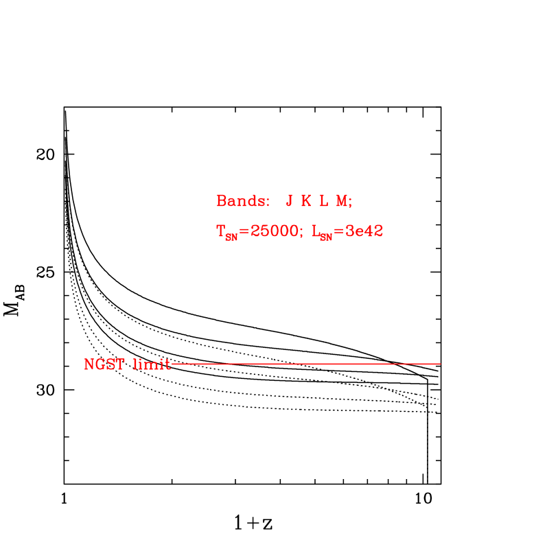
Figure 7: AB apparent magnitude of a SN as a function of its explosion redshift in the four wavelength bands J, K, L, M (from the uppermost to the lowermost curve) for the SCDM model. The case for a moderate ($\mu=3$) magnification (solid curves) is compared to the one in which magnification is neglected (dotted). The NGST flux limit is also shown; the vertical line at high redshift in the J band is due to intergalactic absorption.

Fig. 7 shows the AB apparent magnitude of a SN as a function of its explosion redshift in four wavelength bands (J, K, L, M) in the assumed NGST sensitivity range, and we compare it with the instrument flux limit. Note that we have taken into account absorption by the IGM at frequencies higher than the hydrogen Ly$\alpha$ line. The plot also assumes that $T_{SN}=25000$ K, a value corresponding to the temperature approximately appropriate to the first $15(1+z)$ days after the explosion (Woosley & Weaver 1986). After that, the temperature drops to $T\simeq 6000$ K, where hydrogen recombines, for the entire duration of the plateau (see below). From an inspection of Fig. 7 we deduce that, without considering GL magnification effects, the J band offers the best perspectives to observe such an object: at the assumed sensitivity limit, NGST should be able to reach $z\approx 4$. Including GL magnification enhances dramatically the observational capabilities. In fact, as one can see from the solid line set of curves in Fig. 7, even allowing for a magnification $\mu=3$ only, which in all models has a magnification probability larger than 10% at high $z$ (see Fig. 5), this pushes the maximum redshift at which SNe can be detected up to $z\approx 9$ in the K band.

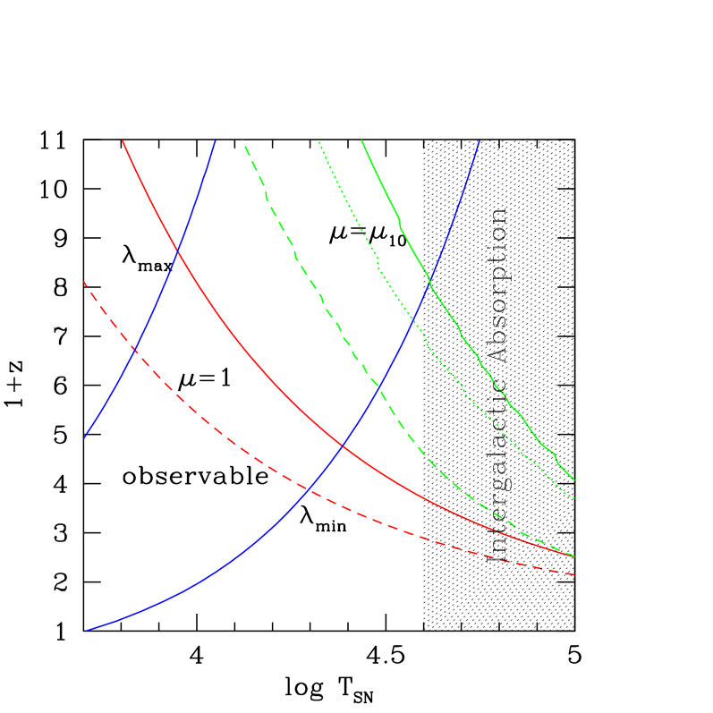
Figure 8: SN detection area (marked as ”observable”) in the redshift-SN temperature, $T_{SN}$, plane neglecting GL magnification (curves $\mu=1$) and with magnification $\mu_{10}(z)$ for the three cosmological models: SDCM (solid curve), LCDM (dashed), CHDM (dotted). Note that for $\mu=1$ the SCDM and CHDM curves overlap. The area is also bound by the lower and upper NGST wavelength limits, $\lambda_{min}$ and $\lambda_{max}$, respectively. The shaded region shows the effect of intergalactic absorption; the SN luminosity is $3\times 10^{42}$ erg s^-1.

A different way to appreciate the GL effects is illustrated by Fig. 8. There we allow for the SN temperature to vary in the large interval $T_{SN}\approx 4000-10^{5}$ K and we ask which is the region of the $(1+z)-T_{SN}$ parameter space in which NGST could possibly detect SNe in primordial objects. This region is constrained by the requirement that the radiation from the SN (or, indicatively, the maximum of its black-body spectrum) falls in between $\lambda_{min}$ and $\lambda_{max}$ with a flux larger than ${\cal F}_{NGST}$. In the absence of magnification, the upper redshift boundary of the detection area (marked as ”observable” in the Figure) is $4<z<8$ for $10^{4}~{}{\rm K}\lower 2.15277pt\hbox{$\;\buildrel<\over{\sim}\;$}T_{SN}\lower 2.15277pt\hbox{$\;\buildrel<\over{\sim}\;$}3\times 10^{4}~{}{\rm K}$ for SCDM and CHDM models (both having $\Omega_{\Lambda}=0$) and $3<z<5.5$ for $8000~{}{\rm K}\lower 2.15277pt\hbox{$\;\buildrel<\over{\sim}\;$}T_{SN}\lower 2.15277pt\hbox{$\;\buildrel<\over{\sim}\;$}2.5\times 10^{4}~{}{\rm K}$ for LCDM. This difference is due to the larger luminosity distance in LCDM models. We can now compare this result with the one obtained considering the GL magnification of the SN, as calculated in the previous Sections. As an indication, we use for $\mu$ the value of $\mu_{10}(z)$ shown in Fig. 5: this quantity should represent a good compromise between the two, usually conflicting, requirements that a high magnification and high probability event occurs. In this case, the upper redshift boundaries (the three uppermost declining curves in Fig. 8) of the detection area are shifted towards higher redshift, in a way that depends on the cosmological models, which are now clearly differentiated because of the concomitant effect of their different $\mu_{10}(z)$ and luminosity distances. Also, the total area is generally increased, thus considerably enhancing the detection chances. The maximum redshift at which a SN can hopefully be observed is now above $z=10$, the limit of our GL simulations, for all models, and it can be extrapolated to $z\approx 12$ for SCDM. The most favorable SN temperature to maximize the depth of the search is $T_{SN}\approx 14000$ K, but a large range, $10^{4}~{}{\rm K}\lower 2.15277pt\hbox{$\;\buildrel<\over{\sim}\;$}T_{SN}\lower 2.15277pt\hbox{$\;\buildrel<\over{\sim}\;$}3\times 10^{4}~{}{\rm K}$, allows to explore the universe illuminated by SNe at redshifts larger than eight. This range is limited at high $T_{SN}$ by integalactic absorption of SN photons above the hydrogen Ly$\alpha$ frequency.

So far, we have emphasized how GL magnification can help us detecting very high-$z$ SNe. However, magnification maps can also contain precious information to discriminate among different cosmological models. There are at least two ways in which one can think of exploiting such information. In principle, the interpretation of SN number counts based on the results shown in Fig. 8 could already provide a first insight on the different properties of the models, since the 10% magnification probability contours are located at different positions. It follows that one would expect different decreasing trends in the number counts with redshift above the $\mu=1$ line. However, this method crucially depends on the star formation/SN production history in the universe; hence a firm interpretation of the results would require a good knowledge of such quantity.

A different, more promising, strategy is instead the reconstruction of the (cumulative) probability distribution, $P(\mu,z)$, shown in Fig. 4. Suppose that, by monitoring a given field (the planned NGST field of view has a size $240\times 240$ arcsec, very similar to the $294\times 294$ arcsec maps shown in Fig. 3) at some appropriate time interval that depends on redshift, a statistically significant number of SNe are discovered following their light curves. From the spectral energy distribution, say in the J K L M bands, and assuming a black body spectrum for the SN, one can determine the ratio $(1+z)/T$. If follow-up spectroscopy is available, the redshift (and, consequently, the temperature) can be determined straightforwardly. However, even if this measure is not possible, one can try a different strategy based on the fact that the light curve is stretched by a factor $(1+z)$. It is well known that Type II SNe fall essentially in two categories, characterized by the presence of a luminosity plateau (SNeII-P) or by an almost linear luminosity decrease (SNeII-L). The duration of the plateau in SNeII-P has a distribution which is peaked around the mean value $70$ days. Hence, lacking a better estimate, the redshift can be determined directly by properly sampling the light curve. Obviously, the accuracy of this method cannot compete with a spectroscopic determination. Nevertheless, there is a fortunate coincidence inherent to the properties of the magnification pattern that makes this error not so crucial when comparing different cosmological models. In fact, we see that for redshift $z\lower 2.15277pt\hbox{$\;\buildrel>\over{\sim}\;$}5$ the $P(\mu,z)$ curves approach a ”limiting” curve (see Fig. 6), i.e. there is no magnification evolution, appropriate for each model. This is due to the fact that in hierarchical models objects present at such high $z$ essentially do not contribute to further magnification because of their low mass. It follows that, even if the redshift is not very precisely known we can still reconstruct $P(\mu,z)$ to a very good accuracy by binning together all the detected SNe with $z\lower 2.15277pt\hbox{$\;\buildrel>\over{\sim}\;$}5$. This is clearly an advantage of the magnification method with respect to the standard direct methods based on the luminosity distance for which a precise determination of the redshift is crucial, as far as discriminating among cosmological models is concerned. The final step is represented by the determination of the absolute luminosity of the plateau phase from which the magnification follows directly. Again we are facing the fact that Type II SNe are not proper standard candles: althoug the plateau luminosity is observed to vary only by a factor $\approx 2$, there are exceptions to this rule (Patat et al. 1994). With this note of caution, we can have at least a first estimate of the magnification.

We conclude this Section by mentioning that Type II SNe have also been used as distance indicators via the so-called Expanding Photosphere Method (Kirshner & Kwan 1974, Montes & Wagoner 1995), which has been rather successful in distance determinations of closer SNe; this technique has recently been adapted for application to moderate redshift SNe (Schmidt et al. 1994a). In short, the luminosity distance (and hence constraints on cosmological models) can be obtained from the formula

$$D_{L}(z)=\sqrt{{\zeta_{\lambda}^{2}\pi R^{2}B_{\lambda}(T)\over\mu(z)f_{\lambda}}},$$ (21)

where $T$ is the SN’s observed color temperature, $\mu(z)f_{\lambda}$ is the observed magnified flux density, $B_{\lambda}(T)$ is the Planck function and $\zeta_{\lambda}$ is a distance correction factor derived from models to account for the dilution effects of scattering atmospheres; the photosperic radius, $R$, can be obtained from optically thin lines and considering free expansion of the ejecta; for this reason, spectral data are necessary (Schmidt et al. 1994b). Thus, this method is suitable for redshift low enough that $\mu(z)\approx 1$; for the redshifts of interest here, a model for the flux magnification has to be nevertheless assumed.

7 Discussion and Summary

In this paper we have explicitly calculated the flux magnification of distant sources due to gravitational lensing effects of the intervening matter distribution in the universe for different cosmological models. We have particularly concentrated on Type II SNe, since at very high $z$ they are likely to offer the best detection perspectives, thus giving us a clue on the star/galaxy formation history in the young universe.

We now discuss briefly the approximations and assumptions made. We have assumed that the lenses are point masses. Although this approximation is commonly used in GL problems and numerical simulations (Schneider & Weiss 1988) due essentially to its simplicity, it remains an idealization of the true lens matter distribution. In reality, even maintaining the less restrictive spherical symmetry hypothesis, lenses are more likely to be extended objects with a given radial density profile. Often, this is taken to be an isothermal profile, since this distribution tends to reproduce reasonably well the properties of galaxy clusters (Narayan & Bartelmann 1997) or leads to a good agreement between COBE data and CDM cosmological models (Kochanek 1995). It is well known (Vietri 1985) that an isothermal sphere has generally a lower magnification power at high magnifications than a point-like lens of the same total mass. Thus, the magnifications we find could be overestimated by some factor, which depends on the redshift of the source. The magnitude of such effect is hard to estimate since we are considering a thick gravitational lens and it is not obvious how the magnification is modified with respect to the single object case, for which this factor is typically $<10$, depending also on the compactness of the lens mass distribution. It has to be pointed out that, in any case, a considerable debate is present in the literature on the detailed shape of dark matter halos. CDM models predict that halo density profiles are essentially self-similar with a weak mass dependence (Lacey & Cole 1994; Navarro et al. 1997); specifically the dark matter density should decrease with radius as $\rho_{h}^{CDM}(r)\propto r^{-1}$ at small radii, down to the resolution of the simulation. Recent observational work, however, appears to disagree with this prediction. Salucci & Persic (1997) have suggested that dark matter halos have a core, i.e. a central region of almost constant density, whose size increases with galaxy luminosity both in absolute units and as a fraction of the optical radius.

The second approximation is the neglect of a possible clustering of the lenses. Since this information cannot be derived directly from the PS formalism used here, an additional hypothesis is necessary to assign the spatial distribution of the lenses on the various planes; as a first step we have adopted a random distribution. Again, reality might be different. Recent works (Hamilton et al. 1991, Matarrese et al. 1997) have been rather successful in reproducing observational data by detailed modelling of the clustering evolution of various populations of objects (QSOs and galaxies). These results are dependent on the bias evolution which is still only partly understood (Mo & White 1996, Kauffmann et al. 1997, Catelan et al. 1997). A detail study of the effects of clustering of galaxies on the magnification distribution function has been carried out by Jaroszyński (1991). From Fig. 4 of that paper, and from the related discussion, it is seen that the differences with respect to a randomly distributed galaxy/lens population are negligible up to values of $\mu\approx 30$. In the high magnification limit, a random distribution leads to a relatively lower probability: for example, for $\mu\approx 100$, $P(\mu)$ is about 3 times smaller in that case. In a subsequent related and more refined work (particularly with a better statistics), Jaroszyński (1992) instead found that the discrepancy between random and correlated lens models are even weaker, and their associated magnification probability distributions would be undistinguishable for flat cosmological models. The likelihood of observing distant supernovae depends only on the magnification probability. As our results have been calculated assuming a magnification with a probability of 10%, typically corresponding to $\mu=2-4$ (see Fig. 5), it follows from the above discussion, that they should not be sensitive to the particular lens spatial distribution adopted. Instead, $P(\mu)$ depends more strongly upon the lens mass distribution, as it is clear from the differences among the three cosmological models studied here. It is interesting to note that in any case as lens correlations tend to enhance high magnification probabilities (Jaroszyński 1992), it will counterbalace to a certain extent the effect of the point-like lens approximation discussed above.

Finally, our description contains two additional hypotheses that should have only a minor effect on the results: (i) the baryonic mass fraction is the same in all lensing objects (ii) we neglect the possible occurrence of microlensing due to stellar mass objects in intervening galaxies.

To conclude the discussion, we comment on our choice of Type II SNe as the primary focus of our efforts. As we have already stated above these events could represent the most distant observable ones in the early universe. This statement is based on the recognition that a SN is expected to be at least 100 times more luminous than their host Pop III object. This is even more true for Type Ia SNe, that are on average brighter by about 1.5 mag; moreover, Type Ia SNe are known to be very good standard candles and, for this reason, they are widely used to determine the geometry of the universe (Garnavich 1997; Perlmutter 1998). Hence, they could be excellent candidates for the present purposes. Unfortunately, it is reasonable to expect that this events at $z\approx 10$ are very rare, since they arise from the explosion of C-O white dwarfs triggered by accretion from a companion; this requires evolutionary timescales comparable with the Hubble time at that redshift. A different possibility would be represented by Type Ib SNe, which originate from short-lived progenitors: however, they share problems similar to Type II SNe, i.e. they are poorer standard candles and are fainter than Type Ia SNe. In any case, our results are valid for all three types of SNe since they give the relative flux enhancement due to GL magnification.

The summary of the main results of this paper, under the assumptions made and discussed above, is the following:

$\bullet$ The magnification patterns are different for the three cosmological models considered: for a given $z$, caustics are more intense and concentrated in SCDM models and their pattern becomes more “grainy” for LCDM and, particularly, for CHDM. Median magnifications are $\simeq 1.5$ for all models.

$\bullet$ The magnification probability function presents a moderate degree of evolution up to $z\approx 5$ (CHDM) and $z\approx 7$ (SCDM/LCDM). All models predict that statistically large magnifications, $\mu\lower 2.15277pt\hbox{$\;\buildrel>\over{\sim}\;$}20$ are achievable, with a probability of the order of a fraction of percent, the SCDM model being the most efficient magnifier. All cosmologies predict that above $z\approx 4$ there is a 10% chance to get magnifications larger than 3.

$\bullet$ We have explored the observational implications of the above results taking NGST, with the planned instrumental characteristics, as a reference instrument. We find that NGST should be able to detect and confirm spectroscopically Type II SNe up to a redshift of $z\approx 4$ in the J band (for $T_{SN}=25000$ K); this limit could be increased up to $z\approx 9$ in the K band, allowing for a relatively moderate magnification. The detection area in the redshift-SN temperature plane depends on cosmological models. When magnification is taken into account, and for the most suitable values of $T_{SN}\approx 14000$ K, the maximum possible detection limit is pushed well above $z=10$. Possibly promising strategies to discriminate among cosmological models using their GL magnification predictions and very high-$z$ SNe are sketched.

We acknowledge C. Kochanek, L. Moscardini, C. Porciani, P. Schneider, M. Vietri for helpful comments.

Figure 1: Fraction of collapsed objects per unit logarithmic mass for various cosmological models with parameters as given in the text: SCDM (solid line), LCDM (dashed) and CHDM (dotted) and for two different redshifts: $z=3$ (light curves) and $z=5$ (thick).

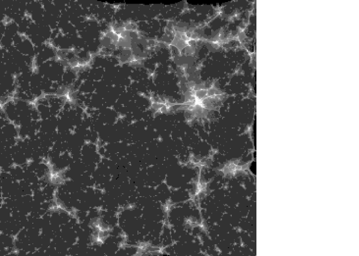
Figure 3: Magnification maps for the three cosmological models: (a) SCDM (b) LCDM (c) CHDM at redshift $z=6$ with symbols defined in the text.

Fig. 3b -

Fig. 3c -

Figure 4: Cumulative magnification probability for four different redshifts $z=3$ (solid line), $z=5$ (dotted), $z=7$ (dashed), and $z=9$ (dot-dashed) for (a) SCDM, (b) LCDM, (c) CHDM models, respectively.

Fig. 4b -

Fig. 4c -

Figure 5: Values of magnification with associated probability larger than 10% as a function of source redshift in the three cosmological models: SCDM (solid line), LCDM (dashed), CHDM (dotted).

Figure 6: Probability associated with magnifications higher than $\mu=10$ as a function of source redshift in the three cosmological models: SCDM (solid line), LCDM (dashed), CHDM (dotted).

References

- (1) Babul, A. & Lee, M.H. 1991, MNRAS, 250, 407
- (2) Bardeen, J.M., Bond, J.R., Kaiser, N., Szalay, A.S. 1986, ApJ, 304, 15
- (3) Brainerd, T.G. & Villumsen, J.V. 1992, ApJ, 394, 409
- (4) Bond, J.R., Cole, S., Efstathiou, G., Kaiser, N. 1991, ApJ, 379, 440
- (5) Carr, B. J., Bond, J. R. & Arnett, W. D. 1984, ApJ, 277, 445
- (6) Carrol, S.M., Press, W.H., Turner, E.L. 1992, ARA&A, 30, 499
- (7) Catelan, P, Lucchin, F., Matarrese, S. & Porciani, C. 1997, MNRAS, in press (astro-ph/9708067)
- (8) Ciardi, B. & Ferrara, A. 1997, ApJ, 483, 5L
- (9) Couchman, H. M. P. & Rees, M. J. 1986, MNRAS, 221, 53
- (10) Dyer, C. C. & Roeder,R. C. 1972, ApJ, 174, 115L
- (11) Efstathiou, G., Bond, J. R. & White, S. D. M. 1992, MNRAS, 258, 1P
- (12) El Eid, M.F.,Fricke, K. J., Ober, W. W., 1983, A&A, 119, 54
- (13) Ferrara, A. 1998, ApJL, in press (astro-ph/9802114)
- (14) Futamase, T. & Sasaki, M. 1989, Fermilab-pub-89/111-A.
- (15) Garnavich, P. M. et al. 1997, ApJ, in press (astro-ph/9710123)
- (16) Gelb, J.M. & Bertschinger, E. 1994, ApJ, 436, 467
- (17) Gnedin, N. Y. & Ostriker, J. P. 1997, ApJ, 486, 581
- (18) Grogin, N. A. & Narayan, R. 1996, ApJ, 473, 570
- (19) Haiman, Z., Rees, M. J., & Loeb, A. 1997, ApJ, 484, 985
- (20) Haiman, Z. & Loeb, A. 1997, ApJ, 483, 21
- (21) Hamilton, A. J. S., Kumar, P., Lu, E. & Mathews, A. 1991, ApJ, 374, L1
- (22) Jaroszyński, M. 1991, MNRAS, 249, 430
- (23) Jaroszyński, M. 1992, MNRAS, 255, 655
- (24) Kashlinsky, A. & Rees, M. J. 1983, 205, 955
- (25) Kauffmann, G., Nussen, A. & Steinmetz, M. 1997, MNRAS, 286, 795
- (26) Kirshner, R. P. & Kwan, J. 1974, ApJ, 193, 27
- (27) Kirshner, R. P. 1990, in ”Supernovae”, ed. A. G. Petschek, (Springer: New York), 59
- (28) Klypin, A., Borgani, S., Holtzman, J., Primack, J. 1995, ApJ, 444, 1
- (29) Kim, A. G. et al. 1997, ApJ, 476, 63L
- (30) Kochanek, C. S. 1995, ApJ, 453, 545
- (31) Kneib, J.-P. 1998, in ”Large Scale Structure: Tracks and Traces”, 12th Postdam Cosmology Workshop, (World Scientific), in press (astro-ph/9711334)
- (32) Lacey, C. & Cole, S. 1994, MNRAS, 271, 676
- (33) Lee, M. H. & Paczyński, B. 1990, ApJ, 357, 32
- (34) Linder, E.V. 1988a, A&A, 206, 175
- (35) Linder, E.V. 1988b, A&A, 206, 190
- (36) Matarrese, S., Coles, P., Lucchin, F. & Moscardini, L. 1997, MNRAS, 286, 115
- (37) Miralda-Escudé, J. & Rees, M.J., 1997, ApJ, 478, 57L
- (38) Mo, H. J. & White, S. D. M. 1996, MNRAS, 282, 347
- (39) Montes, M. J. & Wagoner, R. V. 1995, ApJ, 445, 828
- (40) Nakamura, T.T. 1997, PASJ, 49, 151
- (41) Nakamura, T.T. & Suto, Y. 1997, Prog. Theor. Phys., 97, 49
- (42) Narayan, R. & White, S. D. M. 1988, MNRAS, 231, 97P
- (43) Narayan, R., & Bartelmann, M. 1997, in “Formation of Structure in the Universe”, Proceedings of the 1995 Jerusalem Winter School, eds. A. Dekel & J. P. Ostriker (Cambridge: UniPress), 123
- (44) Navarro, J.F., Frenk, C.S., & White, S.D.M., 1997, ApJ, 490, 493
- (45) Ober, W. W., El Eid, M.F., Fricke, K. J.,1983, A&A, 119, 61
- (46) Palla, F., Salpeter, E. E. & Stahler, S. W. 1983, ApJ, 271, 632
- (47) Patat, F., Barbon, R., Cappellaro, E. & Turatto, M. 1994, A&A, 282, 731
- (48) Peacock, J. A. & Heavens, A. F. 1990, MNRAS, 243, 133
- (49) Perlmutter, S. et al. 1998, Nature, 391, 51
- (50) Porciani, C., Ferrini F., Lucchin, F., Matarrese, S. 1996, MNRAS, 281, 311
- (51) Premadi, P., Martel, H. & Matzner, R. 1997, astro-ph/9708129
- (52) Press, W. H. & Schechter, P. 1974, ApJ, 187, 425
- (53) Salucci, P. & Persic, M. 1997, in Dark and Visible Matter in Galaxies, eds. M. Persic & P. Salucci, ASP Ser. 117, 1
- (54) Schmidt, B. P. et al. 1994a, AJ, 107, 1444
- (55) Schmidt, B. P. et al. 1994b, ApJ, 432, 42
- (56) Seitz, S. & Schneider, P., 1994, A&A, 287, 349
- (57) Seitz, S., Schneider, P. & Ehlers, J. 1994, Class. Quant. Grav., 11, 2345
- (58) Schneider, P., Ehlers, J., Falco, E.E., 1992, Gravitational Lenses, Springer-Verlag, Berlin
- (59) Schneider, P. 1997, MNRAS, 292, 673
- (60) Schneider, P., & Weiss, A. 1988, ApJ, 330, 1
- (61) Shapiro, P. R., Giroux, M. & Babul, A. 1994, ApJ, 427, 25
- (62) Silk, J. 1977, ApJ, 211, 638
- (63) Tegmark, M., Silk, J., Rees, M.J., Blanchard, A., Abel, T. & Palla, F. 1997, ApJ, 474, 1
- (64) Vietri, M. 1985, ApJ, 293, 343
- (65) Wambsganss, J. 1990, ”Gravitational Microlensing”, MPA Report 550, Garching
- (66) Wambsganss, J., Cen, R., Ostriker, J.P. 1996, astro-ph/9610096
- (67) Woosley, S. E. & Weaver, T. A. 1986, ARA&A, 24, 205
- (68) Yano, T., Nagashima, M., Gouda, N. 1996, ApJ, 466, 1