Time Dilation in the Peak-to-Peak Time Scale of GRBs

Abstract

We present strong evidence of time stretching in the peak-to-peak time scales in the light curves of BATSE Gamma Ray Bursts (GRBs). Extensive tests are performed on artificially dilated bursts to verify that the procedure for extracting the peak-to-peak time scales correctly recovers the stretching of bursts. The resulting robust algorithm is then applied to the 4B GRB database. We derive a stretching factor of $1.92\pm 0.13$ between the brightest burst group ($P>7.7photon\cdot cm^{-2}\cdot s^{-1}$) and the dimmest burst group ($P=1.0\sim 1.4photon\cdot cm^{-2}\cdot s^{-1}$) with several independent peak-to-peak time scale definitions and they agree within uncertainties. Such an agreement strongly supports the interpretation of the observed time stretching as time dilation caused by the cosmological expansion, rather than physical selection effects. We fit the result to cosmological models with $\Lambda=0$, $\Omega_{0}$ from 0.2 to 1.0, and contrained the standard candle luminosity to be $L_{0}=7.0\pm 2.0\pm 2.7\times 10^{56}photons\cdot s^{-1}$. Our luminosity value is fully consistent with the value from the combined PVO and BATSE LogN-LogP curve with the BATSE bright bursts at low redshifts of $z_{bright}=0.11\pm 0.02\pm 0.025$. This luminosity fit is definitely inconsistent with the the larger distance scale implied from associating burst density with star formation rates.

1 Introduction

Observations taken by the BATSE instrument aboard the Compton Gamma Ray Observertory have identified $\sim 1800$ GRBs and shown that their angular distribution is highly isotropic, and their distribution in space is inhomogeneous (Meegan et al. 1992, Briggs et al. 1996). Such a distribution naturally arises if GRBs are at cosmological distances. The logN-LogP distribution of GRBs is well studied and shown (e.g. Fenimore et al. 1993) to be consistent with cosmological models. The recent measurement of the redshift of GRB970508 (Metzger et al. 1997) between $0.835\sim 2.1$, and the possible identification of the host galaxy of GRB971214 (Kulkarni et al. 1998) at $z\sim 3.42$ provide further evidence supporting the cosmological scenario.

Piran (1992) and Paczyński (1992) suggested that the light curves of the GRBs should be stretched due to the cosmological time dilation. This effect applies to all time scale in the GRB lightcurves. In the past, different groups (Norris et al. 1994; Mitrofanov et al. 1996; Bonnel et al. 1996; Rutledge et al. 1996 ) have investigated the correlation of the duration of bursts ($T_{50}$ , $T_{90}$, width of the main peak) and the burst brightness (peak flux). The results have been contradictory, with different groups getting different results using identical method and similar data sets.

Furthermore, questions have been raised whether the time stretching found is due to intrinsic correlation (Brainerd 1994, 1997) between pulse width and burst brightness for bursts drawn from a volume limited sample. It is argued that the observed correlation could arise either from the beaming of relativistic jets (Brainerd 1994), or the conservation of total energy in monoenergetic sources (Wijers & Paczyński 1994). Thus the controversial claims of temporal stretching need neither imply cosmological distances nor be of any utility in understanding burst demographics.

In this Letter, we investigate the correlations of the time intervals between peaks with brightness indicators peak flux P. The peak-to-peak time scale is independent of earlier pulse width measurements. Attempts (Pozanenko et al. 1997, Norris et al. 1996) have been made to search for peaks separated by a valley with intensity difference of at least $4\sigma$. Such a definition is biased towards identifying more peaks in the bright bursts than in the dimmer bursts since the latter have less photon counts above background. We used artificially stretched bursts to identify a peak-to-peak time scale which correctly recovers the input stretching relations.

2 Peak Finder Algorithm

We have used the updated BATSE 64ms ascii database which contains 1252 bursts ranging from trigger 105 to trigger 5624. This database provides 64ms time bins from the concatenation of three standard BATSE datatypes, DISCLA, PREB and DISCSC. All three data types are derived from the on-board data stream of BATSE’s eight Large Area Detectors (LADs), and all three data types have four energy channels, with approximate channel boundaries: $25-55keV$, $55-110keV$, $110-320keV$, and $>320keV$ (see Fishman et al. 1989). The peak flux values are derived on the $256ms$ time scale as in the 4th BATSE catalog.

The data were binned to 256ms to achieve better S/N ratio for the dim bursts. Bursts with $T_{90}$ shorter than 2s are excluded (Norris et al. 1994, Mitrofanov et al. 1996) from our analysis. The noise biases are rendered uniform (Norris et al. 1994) by diminishing the background subtracted signal to a canonical peak intensity of $2400counts\cdot s^{-1}$, and adding a canonical flat background of $8000counts\cdot s^{-1}$. The elimination of bursts with peak flux below the $1.0photon\cdot cm^{-2}\cdot s^{-1}$ threshold is introduced to avoid trigger threshold effects and ensure the statistical significance of the peaks identified.

The detailed procedure to find all the peaks in a burst is as follows: (1) We fit the background using a quadratic function to the pre- and postburst regions. The background is subtracted from the data. (2) The maximum peak counting rate $C_{max}$ at 256ms is identified. (3) Identify all local maximums $C_{p}$ that are separated by local minimums $C_{min}$ which satisfy $C_{p}-C_{min}>N_{v}\cdot C_{max}$. (4) Each such local maximum also has to be greater than a threshold level, $C_{p}>T\cdot C_{max}$. $N_{v}$ is a parameter to ensure the peaks are distinct enough statistically. $T$ is a threshold level for accepting a local maximum as a significant peak.

We used four definitions of peak-to-peak time scales. The first method uses all time intervals between successive peaks, $\tau_{i}$. Thus a burst with N peaks will provide N-1 peak-to-peak time scales, all of which have equal weight. Our second method is to logarithmically average all the time intervals between successive peaks $\tau_{p-p}$ for each individual burst, resulting in one time scale per burst. Our third method is to consider only the time interval $\tau_{HS}$ between the highest and the second highest peak. The fourth method is to consider the time interval $\tau_{FL}$ between the first and the last peaks identified.

3 Simulation Tests

The intervals between peaks for long bursts ($T_{90}>2s$) varies from less than 1 second to tens of seconds, thus any dilation effect can be detected only in a statistical sense. Furthermore, the identification of peaks are complicated by small S/N ratios in weak bursts which might introduce noise peaks. The highly significant peaks do not suffer from these problems, while having more peaks identified will improve the statistics of our analysis. Therefore, it is not known a priori which parameters $N_{v}$ and $T$ are the best choice to measure the time intervals between peaks of GRBs, nor do we have a priori knowledge of which peak-to-peak time scale definition yields reliable results. A faithful procedure should be able to distinguish the time stretching effect from any systematic effects.

To find a faithful procedure, we simulated the time stretching effects of the bursts and tested whether our procedure of using the peak finder algorithm in extracting the time scale correctly recovers the time stretching despite the systematic effects. Our procedure is to search the parameter space for $N_{v}$ and $T$ to find regions where the peak finder algorithm recovers the input dilation with high confidence. The details of the simulation procedure go as follows:

We assume a standard cosmology with $\Lambda=0,\Omega_{0}=2q_{0}$. Hence there is the following relationship between peak flux and redshift.

$$P(z)=\frac{5.2\times 10^{-58}\cdot q_{0}^{4}\cdot(1+z)^{-\alpha+2}\cdot L}{[zq_{0}+(q_{0}-1)(\sqrt{2q_{0}z+1}-1)]^{2}}$$ (1)

Here $q_{0}$ is the deceleration parameter, $\alpha$ is the power law spectral index of GRBs, $L$ is the burst luminsity in $photons\cdot s^{-1}$. In deriving this relationship, we assumed a Hubble constant of $75km\cdot s^{-1}\cdot Mpc^{-1}$. The power law spectral index varies from 1.0 to 3.0 for a majority of the bursts (Schaefer et al. 1994). We assumed $q_{0}=0.5$, $\alpha=2.0$, and a typical (Horack et al. 1996, Hakkila et al. 1996) GRB power law luminosity function $\phi(L)=A_{0}L^{-\beta}$ ($L_{min}<L<L_{max}$, $K=L_{max}/L_{min}=100.0$) with $\beta=2.0,L_{min}=2.3\times 10^{57}photons\cdot s^{-1}$ in the simulation process of stretched bursts.

With this cosmology, we created a database of simulated BATSE light curves. Each burst was simulated to have peak flux value P randomly sampled from the $LogN-LogP$ relation of the 4B catalog, and its luminosity $L$ randomly sampled from the luminosity function $\phi(L)$ assumed. Both of them are sampled using the rejection method (Press et al. 1992). Its redshift $z$ is then determined by Eq. 1. We then randomly select a burst from a library of 100 bright BATSE bursts, and determined its redshift $z_{bright}$ from the above relation. Burst photon counts from the 4 different channels from the Large Area Detectors are redistributed by a smooth interpolation function to redshift the photon energy. The energy shift factor is $\epsilon=(1+z_{bright})/(1+z)$.

For the burst at redshift z to be simulated, the relative time dilation factor is $S=\epsilon^{-1}=(1+z)/(1+z_{bright})$. The light curve is then stretched by a factor of S. The photon count of $ith$ bin $N_{i}$ in the stretched light curve is dependent upon the photon count of two bins $O_{p}$ and $O_{p+1}$ in the original light curve, where $p$ is the integer portion of $i/S$. The fraction of $O_{p+1}$ that will contribute is $f=i-p\cdot S$ ($f=1.0$ if $i-p\cdot S>1.0$). Taking account of the new background, the new count $N_{i}$ should be:

$$N_{i}=O_{p+1}\cdot f+O_{p}\cdot(1-f)+p(d),d=O_{p+1}\cdot f^{2}+O_{p}\cdot(1-f)^{2}$$ (2)

where p(d) is a Poisson variable whose standard deviation is $d^{1/2}$. The resulting light curve is then dimmed by a factor of $P(z)/P(z_{bright})$ as prescribed by Norris et al. 1994.

This process is repeated 1250 times to generate a simulated database of gamma ray burst light curves, with the same $LogN-LogP$ distribution as the real 4B GRB database. Each database simulation is repeated 10 times with different seeds for random number generation. By looking at the scatter between these 10 simulations we estimate the uncertainty associated with the simulation procedure.

The peak finder algorithm is applied to each simulated database. We divide the bursts into 6 brightness bins with equal numbers of bursts, and logarithmically averaged the individual peak-to-peak times within each bin. The average peak-to-peak time scales derived are normalized to that of the brightest bin. The resulting relation is then compared to the input dilation relationship of Eq. 1 by a $\chi^{2}$ test. The $\chi^{2}$ values were calculated for a wide range of $N_{v}$ and $T$.

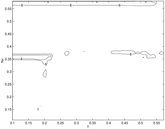
Figure 1: The $\chi^{2}$ contour of the peak-to-peak algorithm for cosmological model with $L_{0}=2.3\times 10^{57}photons\cdot s^{-1}$ . There are two level of $\chi^{2}$s, 4 and 6. The x and y axis are $T$ and $N_{v}$ values respectively. The $\chi^{2}$ values are calculated by fitting $\tau vs.P$ relation recovered by the algorithm to the input stretching relation of 6 burst brightness groups. There are 4 degrees of freedom for the fit, hence the region within $\chi^{2}=4$ provides a faithful algorithm which correctly recovers the input stretching relation.

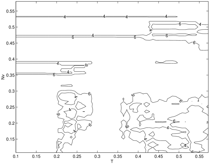
Figure 2: The $\chi^{2}$ contour of the peak-to-peak algorithm for no dilation model. There are two level of $\chi^{2}$s, 4 and 6. The x and y axis are $T$ and $N_{v}$ values respectively. The $\chi^{2}$ values are calculated by fitting $\tau vs.P$ relation recovered by the algorithm to the input stretching relation of 6 burst brightness groups. There are 4 degrees of freedom for the fit, hence the region within $\chi^{2}=4$ provides a faithful algorithm. Notice that the faithful areas are much larger in this case.

In Fig. 1, the $\chi^{2}$ dependency on $N_{v}$ and $T$ is shown by a contour plot for the simulation with the stretching relation of Eq. 1. We also performed simulations for bursts with no stretching, the $\chi^{2}$ dependency on $N_{v}$ and $T$ is shown in Fig. 2. The contour areas that reside within $\chi^{2}=4$ in each figure provide $N_{v}$ and $T$ values that define a peak-to-peak time scale which faithfully recovers the input relation. Obviously, such areas are much larger when we have no stretching (Fig. 2). The overlapping areas ($N_{v}\sim 0.37,T<0.22$) provide a definition that reproduce the dilation relation with high confidence for both the stretched and unstretched simulated database. We repeated the simulation with a variety of cosmological parameters and luminosity values and found that such a conclusion consistently holds. In Table 1, the time stretching relation recovered from the algorithm is compared to the input relation. These simulation procedures ensure that we have a peak-finding algorithm which faithfully returns the stretching factors regardless of the size of stretching.

The primary parameter that ensures the peaks found are nonstatistical is $N_{v}$. It is defined to be the peak-to-valley amplitude (measured in units of the highest peak height above background) separating each candidate peak from its neighbors. When $N_{v}$ is small, the algorithm picks up many statistical fluctuations as peaks, which distort the stretching relation. When $N_{v}$ is large, very few peaks are identified, and the statistics are poor. Nevertheless, these few peaks will result in large uncertainties if they are used as a measurement of $\tau_{i}$ such that $\tau_{i}$ vs. $P$ relation can be fitted to any model with a reasonable $\chi^{2}$. In figures 1 and 2, this is evidenced by a region of $\chi^{2}<6$ across the top for large $N_{v}$ values. While faithful, these regions carry little information as to distinguish between models. Therefore the algorithm only works for intermediate $N_{v}$ values.

The parameter $T$ in the algorithm is defined to be a threshold level that all peaks identified have to exceed. When $N_{v}>T$, the $T$ constraint is primarily important to reject some large statistical fluctuations above and below the background. Although rare, such fluctuations usually yield a peak in the background data far away from the burst activity, creating large $\tau_{i}$ values that are false and distort the apparent $\tau_{i}$ vs. $P$ relation.

4 Results and Conclusions

We applied the algorithm to the real BATSE database, and the result is shown in Fig. 3. A stretching factor $S$ is calculated by fitting the resulting $\tau vs.P$ relationship to Equation 1. The same procedure for simulation test is repeated for the other definitions of peak-to-peak time scales and the resulting algorithm is applied to the real BATSE bursts. The results are summarized in Table 2. The time stretching factor $S$ of $1.92\pm 0.13$ between the brightest ($P>7.7photon\cdot cm^{-2}\cdot s^{-1}$) and dimmest group ($P=1.0\sim 1.4photon\cdot cm^{-2}\cdot s^{-1}$) is found. Within the uncertainties, the different definitions of the peak-to-peak time scales give consistent results.

Recently, two spectral class of bursts have been identified (Pendleton et al. 1997): those bursts with high energy emission (HE), and those with no high energy (NHE) emission. The latter group is predominantly fainter than HE bursts and is found to have a homogeneity to much lower flux values. We applied the peak finder algorithm (see Table 3) to this subgroup with 232 bursts in the 3B catalog. Since the NHE bursts are inherently much fainter, there are fewer bursts with peak flux P above the $1.0photon\cdot cm^{-2}\cdot s^{-1}$ threshold (66 out of 232) and hence the uncertainties are much larger. The time stretching factors of the NHE bursts appears to be consistent with those of the HE bursts (reduced $\chi^{2}_{5}=1.01$) and those of a no stretching model (reduced $\chi^{2}_{5}=1.11$). Therefore, it is safe to conclude that the limited statistics available is not enough to determine whether any stretching exist in NHE bursts.

It should be noted that the time dilation relation is independent of the GRB density evolution. We fit the result to the Eq. 1 and constrain the luminosity value $L_{0}$ in a standard candle scenario. This provides an estimate of the redshift $z_{bright}$ of brightest BATSE bursts independent of previous estimates from the $LogN-LogP$ relation. We fit the data with varying values of deceleration parameters $q_{0}$ from $0.1$ to $0.5$, and power index of GRB spectra $\alpha$ from $1.0$ to $2.0$. We find the best fitting luminosity $L_{0}=7.0\pm 2.0\pm 2.7\times 10^{56}photons\cdot s^{-1}$ (reduced $\chi^{2}_{4}=1.23$), and the brightest bursts (peak flux $P=30photons\cdot cm^{-2}s^{-1}$) at $z_{bright}=0.11\pm 0.02\pm 0.025$. The first error denotes the uncertainty associated with the varying values of $q_{0}$ and $\alpha$, the second error is derived from the $\chi^{2}$ fits. This result favors the simple cosmological scenario of bright bursts at small redshifts rather than evolutionary scenario of bursts at much larger redshifts based on some theoretical arguments (Totani 1997, Paczyński 1997) that burst density traces star formation rates.

It is well known that GRBs might have a broad luminosity function. We performed our simulation adopting a range dominated luminosity model (Horack 1996, Hakkila 1996) and demonstrated that for typical luminosity function $\phi(L)\propto L^{-\beta}$ ($L_{min}<L<L_{max}$, $K=L_{max}/L_{min}=100.0$) with power-law index $\beta$ near 2, the broadening of the luminosity distribution will not smear the time dilation effect out. Our simulation shows that our technique can correctly recover the time stretching on a bright burst sample for this case. However, the time dilation data alone can not be used to constrain all the parameters $L_{min},L_{max},\beta$ in the power law luminosity function as it involves too many free parameters in the cosmological model.

In summary, we have measured several peak-to-peak time scales of GRBs. Simulation tests are performed to verify that the time scales identified correctly reflect the physical time scale intrinsic to the bursts. The $\tau_{HS}$ and $\tau_{FL}$ time scales are similar to the durations, while the $\tau_{i}$ and $\tau_{p-p}$ peak-to-peak time scales measurements are independent of previous duration and pulse width measurements. Our result unambiguously shows the existence of time stretching factor of $s=1.92\pm 0.13$ between the bright and dimmest GRB time profiles, and the agreement found between these multiple independent time scale measurements indicates that the temporal profiles of GRBs are universally stretched. Such an agreement implies that the time stretching relation comes from cosmological expansion rather than physical selection effects affecting particular property of bursts.

We thank G. N. Pendleton for providing the list of NHE bursts. This work has made use of the data obtained though the Compton Gamma Ray Observatory Science Support Center Online Service, provided by the Goddard Space Flight Center.

$P(photons\cdot cm^{-2}\cdot s^{-1})$	$s_{Nodilation}$	$s_{recovered}$
$1.0\sim 1.4$	1.00	$1.04\pm 0.10$
$1.4\sim 1.8$	1.00	$1.05\pm 0.09$
$1.8\sim 2.5$	1.00	$1.13\pm 0.09$
$2.5\sim 3.6$	1.00	$0.98\pm 0.08$
$3.6\sim 7.7$	1.00	$1.10\pm 0.09$
$>7.7$	1.00	$1.00\pm 0.09$
$P(photons\cdot cm^{-2}\cdot s^{-1})$	$s_{Dilation}$	$s_{recovered}$
$1.0\sim 1.4$	1.69	$1.82\pm 0.12$
$1.4\sim 1.8$	1.56	$1.67\pm 0.09$
$1.8\sim 2.5$	1.44	$1.58\pm 0.11$
$2.5\sim 3.6$	1.30	$1.28\pm 0.12$
$3.6\sim 7.7$	1.17	$1.12\pm 0.11$
$>7.7$	1.00	$1.00\pm 0.08$

Table 1: The input stretching factor and the measured factor using the definition of peak-to-peak time scales $<\tau_{p-p}>$ with $N_{v}=0.375$ and $T=0.100$ for both simulated stretched bursts and unstretched bursts.

Peak-to-peak Timescale	Stretching Factor
Definition	$s_{observed}$
$\tau_{i}$	$1.92\pm 0.13$
$<\tau_{p-p}>$	$1.96\pm 0.17$
$\tau_{HS}$	$1.92\pm 0.26$
$\tau_{FL}$	$1.92\pm 0.20$

Table 2: The observed time stretching factor between the brightest burst group ($P>7.7photon\cdot cm^{-2}\cdot s^{-1}$) and the dimmest burst group ($P=1.0\sim 1.4photon\cdot cm^{-2}\cdot s^{-1}$) using different definition of time scales.

$P(photons\cdot cm^{-2}\cdot s^{-1})$	$s_{NHE}$	$s_{HE}$	$s_{All}$
$1.0\sim 1.4$	$1.68\pm 0.49$	$1.83\pm 0.23$	$1.92\pm 0.24$
$1.4\sim 1.8$	$2.97\pm 1.28$	$1.56\pm 0.22$	$1.65\pm 0.20$
$1.8\sim 2.5$	$0.90\pm 0.28$	$1.40\pm 0.18$	$1.27\pm 0.16$
$2.5\sim 3.6$	$1.54\pm 0.60$	$1.24\pm 0.14$	$1.42\pm 0.16$
$3.6\sim 7.7$	$1.40\pm 0.70$	$1.03\pm 0.12$	$1.08\pm 0.13$
$>7.7$	$1.00\pm 0.29$	$1.00\pm 0.10$	$1.00\pm 0.09$

Table 3: The stretching factor relative to the brightest burst group for NHE bursts, HE bursts and all the bursts. Notice that the uncertainties associated with the NHE bursts are substantially larger due to the relative scarcity of such events in the 4B catalog.

Figure 3: The average peak-to-peak intervals of BATSE GRB database. Each dot in the graph represents the peak-to-peak interval identified $\tau_{i}$ in a mutipeak burst. P is the peak flux in $photons\cdot cm^{-2}\cdot s^{-1}$. $\tau_{i}$ is the peak-to-peak interval in units of seconds. The solid curve is the best fit to a cosmological model with $q_{0}=0.2$, $\Lambda=0$, $\alpha=1.5$, and burst standard candle luminosity $L_{0}=7.0\pm 2.7\times 10^{56}photons\cdot s^{-1}$.

References

- (1) Brainerd J. J., 1994, ApJ, 428, 21
- (2) Brainerd J. J., 1997, ApJ, 487, 96
- (3) Briggs M. S., et al. 1996, ApJ, 459, 40
- (4) Fenimore E. E., et al. 1993, Nature, 366, 40
- (5) Fishman G. J., 1989, in Proc. Gamma Ray Observatory Science Workshop, ed. W. N. Johnson(Greenbelt, MD: NASA/GSFC), 2-39
- (6) Hakkila J. et al. 1996, ApJ, 462, 125
- (7) Horack J. M. et al. 1996, ApJ, 462, 131
- (8) Kulkarni S. R. et al. 1998, Nature, 393, 35
- (9) Meegan C. A. et al. 1992, Nature, 355, 143
- (10) Metzger M. R. et al. 1997, IAU Circ. 6655
- (11) Mitrofanov I. G. et al. 1994, AIP Conf. Proc. 307, Gamma-Ray Bursts: 2d Huntsville Symp., ed. G. J. Fishman, J. J. Brainerd, & K. Hurley(New York:AIP), 187
- (12) Mitrofanov I. G. et al. 1996, ApJ, 459, 570
- (13) Norris J. P. et al. 1994, ApJ, 424, 540
- (14) Norris J. P. et al. 1996, AIP Conf. Proc., 384, Gamma-Ray Bursts: 3d Huntsville Symp., ed. C. Kouveliotou, M. Briggs, & G. Fishman(New York:AIP), 77
- (15) Paczyński B., 1992, Nature, 355, 521
- (16) Paczyński B., 1997, astro-ph/9710086
- (17) Pendleton G. N. et al. 1997, ApJ, 489, 175
- (18) Piran T., 1992, ApJ, 389, L45
- (19) Pozanenko A. S. et al. 1997, in press, Gamma-Ray Bursts: 4th Huntsville Symp.
- (20) Press et al., 1992, Numerical Recipes in Fortran (Cambridge University Press), 281
- (21) Rutledge R. E. et al. 1996, AIP Conf. Proc., 384, Gamma-Ray Bursts: 3d Huntsville Symp., ed. C. Kouveliotou, M. Briggs, & G. Fishman(New York:AIP), 527
- (22) Schaefer et al. 1994, ApJS, 92, 285
- (23) Totani T., 1997, ApJ, 486, L71
- (24) Wijers R. A. M. J., & Paczyński, B. 1994, ApJ, 437, L107