Shell formation and star formation in superbubble DEM 192
Accepted 28-05-98 to the Astronomical Journal

Abstract

Was star formation in the OB associations, LH 51 and LH 54, triggered by the growth of the superbubble DEM 192? To examine this possibility, we investigate the stellar contents and star formation history, and model the evolution of the shell. H-R diagrams constructed from $UBV$ photometry and spectral classifications indicate highly coeval star formation, with the entire massive star population having an age of $\lesssim$ 2–3 Myr. However, LH 54 is constrained to an age of $\sim$ 3 Myr by the presence of a WR star, and the IMF for LH 51 suggests a lower-mass limit implying an age of 1–2 Myr. There is no evidence of an earlier stellar population to create the superbubble, but the modeled shell kinematics are consistent with an origin due to the strongest stellar winds of LH 54. It might therefore be possible that LH 54 created the superbubble, which in turn may have triggered the creation of LH 51. Within the errors, the spatial distribution of stellar masses and IMF appear uniform within the associations.

We reinvestigate the estimates for stellar wind power $L_{w}(t)$, during the H-burning phase, and note that revised mass-loss rates yield a significantly different form for $L_{w}(t)$, and may affect stellar evolution timescales. We also model superbubble expansion into an ambient medium with a sudden, discontinuous drop in density, and find that this can easily reproduce the anomalously high shell expansion velocities seen in many superbubbles.

M. S. Oey and S. A. Smedley Shell and Star Formation

and

1 Introduction

As early as the work of Bok, Bok, & Basinski (1962), the OB associations LH 51 and LH 54 (Lucke & Hodge 1970) in the Large Magellanic Cloud (LMC) have been recognized as an extremely young star-forming region. However, the complex is especially notable for its associated superbubble, which is one of the most prominent such objects in the LMC that is seen in H$\alpha$ (e.g., Meaburn 1980). This nebula has been cataloged in H$\alpha$ surveys of the LMC as DEM 192 (Davies, Elliott, & Meaburn 1976) and N51 D (Henize 1956). Figure 1 shows images kindly obtained by R.C. Smith with the U. Michigan/CTIO Curtis Schmidt Telescope, in the light of H$\alpha$ (Figure 1$a$, Plate *) and [S 2] (Figure 1$b$, Plate *). Interestingly, the young, massive stars are not centered within the the superbubble, but are located toward the east and west edges of the nebular shell. The geometry of the complex is therefore suggestive of triggered, or propagating star formation induced by the accumulation and compression of gas in the expanding shell.

1$a$

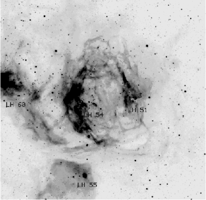
Figure 1: DEM 192 in H$\alpha$, provided by R. C. Smith from the U. Michigan/CTIO Magellanic Clouds Emission-Line Survey.

1$b$

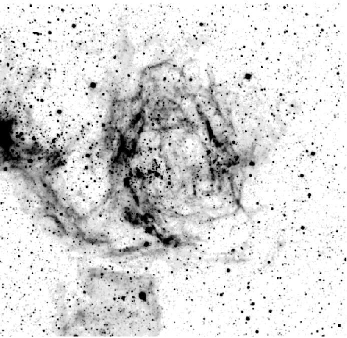
Figure 2: DEM 192 in [S 2], also obtained by R. C. Smith.

Since both OB associations, especially LH 54, are aligned radially with respect to the shell, it is particularly suggestive that star formation may be propagating outward as the superbubble expands. If this were the case, then quantifying the age gradient would be of primary interest in understanding the progression of triggered star formation, as well as confirming superbubble expansion timescales, which are not well-understood (Oey 1996a). We therefore wish to determine the star formation history in this complex, and shell evolution, in relation to each other. This will require a detailed investigation of the stellar population, with subsequent modeling of the superbubble. The stellar data will also allow us to examine the initial mass function (IMF) across the region.

2 Observations

We have presented $UBV$ photometry for 1460 stars in this region in a previous study (Oey 1996b), where a CCD mosaic image of the stellar population may be found, which identifies the visually brightest members. Subsequent spectroscopic observations of the hottest stars were obtained as part of the sample studied by Oey (1996c). The observational details may be found in that paper, so we summarize them only briefly here.

Figure 2: Classification spectra of the visually brightest stars.

The spectra were obtained in 1994 January at the CTIO 4-m Blanco telescope, using the Argus multi-fiber spectrograph. A 632 line mm^-1 grating was used in second order, yielding a wavelength coverage of about 3800–4900 Å. The spectra, having a resolution of $2.2$ Å, were recorded on a Reticon II 1200 $\times$ 400 pixel CCD. After standard CCD reduction procedures, the target observations in each exposure were sky-subtracted with spectra combined from the 24 or more fibers set on sky positions. The target spectra were then rectified and classified according to the criteria of Walborn & Fitzpatrick (1990). A few spectra of the brightest stars are shown in Figure 2$a$ and $b$.

In keeping with the companion study of OB associations, the stellar data were transformed to $M_{\rm bol}$ and $T_{\rm eff}$ according to the prescription in that work (Oey 1996c). For stars with spectral types, we used the $T_{\rm eff}$ calibrations and bolometric corrections of Chlebowski & Garmany (1991) and Humphreys & McElroy (1984). Stars with only photometric data were transformed with the relations given by Massey et al. (1995). As described in Oey (1996c), stars with errors in color $>0.07$ mag have $T_{\rm eff}$ derived from their $B-V$ color alone, while those with more reliable colors use both $B-V$ and $U-B$ to obtain $T_{\rm eff}$. We find a median and mean reddening of $E(B-V)=0.08$ and 0.09, respectively, derived from the 141 stars with combined photometric errors $\lesssim 0.05$ mag. Since the reddening distribution is asymmetric, we adopt the median value for all stars for which $T_{\rm eff}$ was derived from the $B-V$ color only. We use the extinction function of Savage & Mathis (1979), with $A_{V}=3.1\times E(B-V)$ and $E(U-B)=0.66\times E(B-V)$. As in the other papers in this series, we adopted a distance modulus to the LMC of 18.4.

Table 1 presents empirical parameters for the 47 stars in the spectroscopic sample. The stars are identified in the first column, according to the nomenclature of Oey (1996b), where photometric data for the entire sample may be found. In columns 2 and 3, we list the stellar coordinates for epoch J2000.0. Columns 4 – 6 give the photometric data, uncorrected for extinction: $V$, $B-V$ and $U-B$. Columns 7 – 10 give the color excess $E(B-V)$, $\log\ T_{\rm eff}$, $M_{\rm bol}$, and the spectral classification. Three spectroscopic binaries were treated as described in Oey (1996c), and are identified in Table 1 with “a” and “b” notations. Among these is the WC 5 star Br 31 (Sk –67 104), whose $T_{\rm eff}$ and $M_{\rm bol}$ are indeterminate. Its companion had been classified as O9 by Breysacher (1981), and we refine this to O8 Iaf (Figure 2$b$). Three additional binary candidates are noted with the “#” symbol on their spectral classifications. A few bright stars with identifications from other catalogs are cross-referenced in Oey (1996b).

Table 1: Stellar Parameters of Stars with Spectral Types

Star ID	R.A.  (J2000)  Dec.	$V$	$B-V$	$U-B$	$E(B-V)$	$\log T_{\rm eff}$	$M_{\rm bol}$	Sp. Type
L54SA-1b	5 26 04.31   –67 29 58.7	11.418	–0.118	–1.014	0.08	4.53	–10.5	O8 Iaf
L54SA-2	5 26 15.51   –67 30 01.8	11.963	–0.158	–1.048	0.15	4.56	–10.4	O8 III((f))
L54S-2	5 26 20.91   –67 29 57.7	12.674	–0.165	–1.021	0.12	4.51	–9.2	O9 Ib(f)
L51N-1	5 25 15.84   –67 28 06.5	13.019	–0.199	–1.006	0.11	4.54	–9.1	O8.5 III((f))
L54S-1a	5 25 56.57   –67 30 30.1	13.111	–0.187	–1.021	0.08	4.58	–9.2	O7: III(f)
L54S-4	5 26 24.27   –67 30 17.4	13.130	–0.215	–1.010	0.10	4.65	–9.6	O4 III(f*)
L54S-5	5 26 15.80   –67 29 44.3	13.159	–0.173	–1.054	0.14	4.56	–9.1	O8 III((f))
L54S-3a	5 26 08.95   –67 29 47.5	13.311	–0.218	–1.008	0.08	4.61	–9.2	O6.5: V
L54S-3b	5 26 08.95   –67 29 47.5	13.511	–0.218	–1.008	0.08	4.26	–6.7	B2: II:
L54S-1b	5 25 56.57   –67 30 30.1	13.611	–0.187	–1.021	0.08	4.41	–7.5	B0.5: III:
L54N-2	5 26 08.19   –67 28 28.3	13.739	–0.190	–0.979	0.13	4.61	–8.9	O6.5 V
L54N-3	5 26 23.75   –67 29 07.1	13.841	–0.139	–0.928	0.12	4.32	–6.9	B1 IIIe
L54N-4	5 26 05.47   –67 29 07.7	13.909	–0.196	–1.037	0.11	4.56	–8.3	O9 V
L54S-8	5 26 32.16   –67 29 51.3	13.966	–0.178	–0.872	0.04	4.36	–6.6	B0.5 Ib
L51N-3	5 25 31.03   –67 28 38.9	13.992	–0.223	–0.999	0.09	4.56	–8.1	O9 V
L54S-9	5 26 20.78   –67 29 52.1	14.066	–0.197	–0.882	0.10	4.48	–7.6	B0 III
L54N-6	5 26 28.13   –67 27 23.1	14.310	–0.189	–0.992	0.12	4.56	–7.9	O9 V
L54S-10	5 26 03.31   –67 32 10.4	14.355	0.045	–1.097	0.30	4.38	–7.5	early B:: +neb
L54N-7	5 26 18.51   –67 26 45.6	14.369	–0.063	–0.963	0.22	4.40	–7.3	B0.5:: V +neb
L51S-2	5 25 28.42   –67 29 13.3	14.418	–0.221	–1.043	0.10	4.63	–8.2	O6 V((f))e
L54SA-4	5 26 15.85   –67 29 49.9	14.472	–0.217	–0.941	0.06	4.41	–6.6	B0.5 III
L54S-12	5 26 04.42   –67 29 35.6	14.624	–0.196	–0.962	0.10	4.47	–7.1	B0 V #
L54S-13	5 26 19.98   –67 30 01.7	14.640	–0.191	–0.896	0.09	4.40	–6.6	B0.5 Ve
L54S-14	5 26 16.85   –67 29 38.0	14.641	–0.197	–0.976	0.10	4.54	–7.5	O9.5 V
L54S-15	5 26 24.13   –67 30 33.6	14.645	–0.222	–1.007	0.09	4.58	–7.6	O8 Ve
L54S-16	5 26 02.91   –67 29 33.2	14.646	–0.237	–0.979	0.06	4.54	–7.3	O9.5 V #
L51S-3	5 25 27.36   –67 29 10.0	14.675	–0.239	–1.019	0.07	4.58	–7.6	O8 V
L51S-4	5 25 35.31   –67 28 56.7	14.688	–0.222	–0.960	0.06	4.40	–6.5	B0.5 V
L54S-18	5 26 14.43   –67 29 34.6	14.692	–0.229	–0.998	0.08	4.56	–7.4	O9 V
L54S-19	5 26 06.45   –67 29 50.7	14.820	–0.114	–1.004	0.17	4.40	–6.7	B0.5: V #
L51S-5	5 25 30.74   –67 29 26.1	14.948	–0.225	–0.953	0.06	4.40	–6.2	B0.5 V
L51N-9	5 25 31.86   –67 26 51.7	14.999	–0.219	–0.909	0.04	4.38	–6.0	B1: V +neb
L51N-10	5 25 32.50   –67 28 37.5	15.041	–0.211	–0.967	0.09	4.47	–6.6	B0 V
L54S-20	5 26 08.51   –67 30 25.6	15.078	–0.199	–1.010	0.10	4.54	–7.0	O9.5 V
L54SA-5	5 26 15.14   –67 30 06.2	15.087	–0.210	–0.815	0.05	4.38	–6.0	B1:: V +neb
L51S-7	5 25 14.19   –67 29 07.0	15.101	–0.203	–0.946	0.10	4.54	–7.0	O9.5 V
L54SA-1a	5 26 04.31   –67 29 58.7	15.118	–0.118	–1.014	0.08			WC 5
L51N-12	5 25 28.17   –67 27 59.0	15.121	–0.218	–0.943	0.06	4.40	–6.1	B0.5 V +neb
L54S-22	5 26 04.20   –67 29 25.5	15.188	–0.156	–0.972	0.14	4.54	–7.0	O9.5-B0 V
L54S-24	5 26 21.81   –67 29 24.2	15.264	–0.211	–0.993	0.09	4.54	–6.8	O9.5 V +neb
L54N-14	5 25 56.15   –67 28 10.5	15.279	–0.204	–0.990	0.10	4.54	–6.8	O9.5 V
L54S-25	5 26 17.93   –67 30 42.5	15.288	–0.190	–0.885	0.06	4.30	–5.1	B1.5 III +neb
L54N-16	5 26 14.25   –67 28 43.6	15.313	–0.196	–0.975	0.10	4.54	–6.8	O9.5 V
L54S-26	5 26 12.42   –67 30 45.1	15.408	–0.197	–0.991	0.06	4.38	–5.7	B1:: V +neb
L54N-18	5 26 08.80   –67 26 34.8	15.461	0.052	–0.903	0.37	4.63	–8.0	O6: Ve
L51S-9	5 25 40.62   –67 30 40.9	15.473	–0.238	–0.919	0.06	4.47	–6.1	B0:: V
L54SA-7	5 26 05.06   –67 29 58.5	15.499	–0.260	–0.735	0.03	4.34	–5.2	B1.5 V
L54N-19	5 26 14.30   –67 27 11.2	15.527	–0.169	–0.993	0.13	4.54	–6.7	O9.5 V
L54N-21	5 25 53.87   –67 26 43.4	15.593	–0.152	–0.797	0.07	4.28	–4.9	B2.5 V
L54S-36	5 26 09.22   –67 31 11.1	15.789	–0.184	–0.967	0.07	4.34	–5.0	B1.5:: Ve
L54N-25	5 26 24.95   –67 28 53.0	15.816	–0.002	–0.854	0.24	4.29	–5.3	B2:: V +neb
L54N-27	5 26 29.30   –67 27 09.9	15.921	–0.149	–0.946	0.15	4.47	–5.9	O9.5-early Be
L51S-14	5 25 21.44   –67 31 26.6	15.960	–0.201	–0.882	0.06	4.38	–5.1	B1:: V
L54N-33	5 25 55.86   –67 27 44.4	16.390	–0.164	–0.939	0.10	4.38	–4.8	B1:: V

3 The Stellar Population and Formation History

Figure 3: Assumed boundaries for ($a$) LH 51 and LH 54; and ($b$) subregions A – E. Point size is assigned according to $M_{\rm bol}$, with bin separations at $M_{\rm bol}=-7,\ -4,$ and $-1$. Panel ($a$) also shows the central region studied in Figure 8$a$. The WC 5 + O8 Iaf binary star, Sk –67 104, is identified by the solid point.

Figure 4: CMDs of $V$ vs. $B-V$ for ($a$) LH 51 and ($b$) LH 54, with isochrones overplotted for 4, 6, and 8 Myr. Point sizes are assigned as in Figure 3. Representative photometric error bars are shown along the left side of Figure 4$a$, at the corresponding $V$ mag.

In Figure 4$a$ and $b$, we show the color-magnitude diagrams (CMDs) of $V$ vs. $B-V$ for LH 51 and LH 54, respectively, as delineated by the boundaries shown in Figure 3$a$. There are four point sizes, assigned according to the derived bolometric magnitude, separated by $M_{\rm bol}$ of –7, –4, and –1. These CMDs show the data uncorrected for reddening, but with the isochrones adjusted for the median $E(B-V)=0.08$. The overplotted isochrones are for 4, 6, and 8 Myr, computed with the code of G. Meynet. We ran this code with the stellar models of Schaerer et al. (1993), which include convective overshooting, and adopt a metallicity of $Z=0.008$, appropriate to the LMC.

The data are remarkable in the extremely narrow locus of the association members, suggesting coeval star formation, low differential reddening, and small photometric errors. This of course does not preclude the effect of systematic uncertainties, which we estimate to be $\lesssim 0.03$ mag for stars with $V\lesssim 17$, dominated by transformation errors and aperture corrections (Oey 1996b). These are included in the error bars shown in Figure 4$a$. At first glance, the CMDs appear to be well-fitted by isochrones up to 6 or 8 Myr. However, it is apparent that only the very brightest stars are positioned to differentiate between the isochrones. The H-R diagrams we construct below will demonstrate that the associations are in fact much younger.

Figure 5: CMDs of $V$ vs. $U-B$ for $(a)$ LH 51 and ($b$) LH 54, with isochrones overplotted.

It is apparent that the relative unreliability of the $B-V$ CMD stems from the degeneracy in $B-V$ colors (e.g., Massey et al. 1995). This can also be seen from the inconsistency in age determinations suggested by the $V$ vs. $U-B$ CMDs (Figure 5). Since $U-B$ is more sensitive to $T_{\rm eff}$ for OB stars, the same isochrones diverge more, allowing a more reliable age determination. A younger isochrone is implied in Figure 5, in order to match the most luminous stars. However, even in these CMDs one can see that the hottest stars are also degenerate in their colors. Furthermore, there appears to be a problem in the $U-B$ isochrones, which may stem from the poor constraints on the UV energy distributions of OB stars. The isochrones in Figure 5 do not match the locus of the stars in the CMD. The difference appears to be roughly 0.2 mag in $U-B$, which is much larger than the typical errors for the stars. While transformation errors are largest in $U$, they do not exceed 0.023 mag, the worst uncertainty among the four nights of observations. The transformations were computed from observations of 12 to 17 standard stars per night. The mismatch in observed and predicted $U-B$ colors has also been reported by other studies (e.g., Will, Bomans, & Dieball 1997; Hunter et al. 1995). Ultimately, more reliable $U-B$ isochrones will naturally be more useful than those in $B-V$.

Figure 6: H-R diagrams for ($a$) LH 51 and ($b$) LH 54. Solid points indicate stars with spectral classifications; open circles show stars placed using $U-B$ and $B-V$ colors; crosses show those placed from $B-V$ only; and triangles show components of spectroscopic binaries. The WR star Br 31 is not shown. Evolutionary tracks (solid lines) are shown for stellar models with the masses indicated, and the isochrones (dashed lines) shown are for 2 (upper), 4 (middle), and 6 Myr (lower).

In Figure 6 we show the physical H-R diagram (HRD) for LH 51 and LH 54, with stellar evolutionary tracks overplotted for the indicated masses (solid lines). We also show isochrones for 2, 4, and 6 Myr with the dashed lines. Stars plotted with solid circles are those with spectral classifications; open circles show those whose parameters were derived from both $U-B$ and $B-V$ colors; crosses show those derived from $B-V$ only; and triangles show components of spectroscopic binaries. The Wolf-Rayet (WR) star Br 31 is not included on the HRDs. From Figure 6, the isochrones now show an age of $\lesssim 4$ Myr for LH 51, and $\lesssim 3$ Myr for LH 54. With this age constraint, the presence of the WR star suggests that LH 54 must be about 3 Myr old (e.g., Schaerer et al. 1993). There is no evidence of any age spread among or between the associations, and no evolved stars below the upper-mass turnoff, as is often seen in other OB associations (Massey et al. 1995). The star formation therefore appears to be coeval to within 2–3 Myr, the lifetimes of the highest-mass stars. However, in §3.2 below, we suggest the possibility of an age differential between LH 51 and LH 54 based on evidence from the IMF.

Figure 7: H-R diagrams for subregions ($a$) A, ($b$) B, and ($c$) C in LH 54; and ($d$) D and ($e$) E in LH 51. Symbols are as in Figure 6.

3.1 Populations in Subregions

Given this limit for coevality of the star formation, it is therefore difficult to infer an age gradient in the superbubble. However, we can examine different subgroups of stars within the associations, to search for possible hints revealed by the spatial distribution of stellar masses. Figure 3$b$ shows the finding chart for groups A, B, and C in LH 54; and groups D and E in LH 51. The HRDs for these regions are shown in Figure 7. The subgroups in LH 54 all show high-mass stars around $60\rm\,M_{\odot}$ or above, and regions D and E in LH 51 both show stars near $40\rm\,M_{\odot}$. Thus the spatial distribution of masses appears to be highly uniform. The age differentials again appear to be no greater than $\sim 2$–3 Myr, and could well be less. These OB associations therefore do not internally exhibit propagating star formation on any greater timescales. This is in marked contrast to star forming complexes like DEM 34, which, like DEM 192, has an associated superbubble, but shows clear age differences among different subgroups (Walborn & Parker 1992).

If the stars were truly coeval, then what would be the origin of the superbubble? It is peculiar that the stars are concentrated toward the edges of the shell, rather than within the center. If LH 51 and LH 54 were born before the superbubble, then presumably we would expect two shells centered on the associations. This is clearly not the case. We suspect that pre-existing geometry of the gas must play a role in the position of the shell, but it is difficult to believe that two separate gas clouds have conspired to create an almost perfectly spherical shell, with fairly well-behaved expansion kinematics (Lasker 1980; Meaburn & Terrett 1980).

One clue may lie in the fact that the western edge of LH 54 is located closer toward the center of the superbubble, where the gas appears relatively cleared out (Figure 1). It may therefore be that the stars on the west side of LH 54 were surrounded by less gas from the natal cloud, therefore initiating the superbubble’s formation around this region. The position of the stars in LH 51 suggests that they have not contributed substantially to the formation of the superbubble. This may be because they younger, within the age constraints found above. We note that LH 51 contains no evolved stars whatsoever, whereas LH 54 contains the WR star Br 31. LH 51 also contains fewer stars, and somewhat lower-mass stars, as is expected from the stochastic nature of the highest-mass star formation in sparser clusters. This association therefore has less stellar wind power to disperse its surrounding gas, although we note that the reddening values for LH 51 actually appear to be slightly lower than those for LH 54.

Figure 8: H-R diagrams for ($a$) the central region defined in Figure 3$a$, and ($b$) the region south of $-67.52^{\circ}$. Evolutionary tracks for stars of 7 and 15 $\rm\,M_{\odot}$ are shown as indicated (solid lines), and the dashed line shows the isochrone for 1 Gyr. Symbols are as in Figure 6.

Could it be that a previous stellar population, more closely centered within the superbubble, is the origin of the shell? In Figure 8$a$, we show the HRD for stars in the central region between LH 51 and LH 54, delineated in Figure 3$a$. Figure 8$b$ shows the HRD for all stars south of $-67.52^{\circ}$, which, lying on the outskirts of the region, should resemble the background population. We do caution that most of this region still appears to be within the confines of the superbubble in projection, but given the fairly concentrated distribution of stars in the OB associations, this area is likely to yield characteristics of the background. There appears to be no significant difference in the HRDs in Figure 8. The highest-mass stars in each population ($7-15\ \rm\,M_{\odot}$) could be members of the OB associations, so the age determinations are not well-constrained. However, both the central region and outskirts suggest ages of several$\times 10^{7}$ yr, with an older, underlying background of red giants with an age of order $\sim 1$ Gyr. This is consistent with the burst in field star formation beginning around 2 Gyr ago (e.g., Vallenari et al. 1996). Given that the younger populations in Figure 8 appear to be similar both in the center and outskirts of the shell, we infer a continuous background with this age of several$\times 10^{7}$ yr, which is therefore unlikely to have spawned the superbubble.

3.2 The Initial Mass Function

We compute the IMF for the OB associations following Massey et al. (1989), where $\xi(\log m)$ is defined as the number of stars per logarithmic mass interval per kpc². Assuming coeval star formation as suggested above, the present-day mass function reflects the IMF. The evolutionary tracks for the different masses are used to define the mass bins for the stellar census (Figure 6), where the tracks define the bin limits. We then correct for the bin size and spatial area for each region defined in Figure 3 to obtain $\xi(\log m)$, for all stars with masses $>7\ \rm\,M_{\odot}$. We computed the slope $\Gamma$ with a least-square polynomial fit, weighted by root-$N$ in each bin.

Figure 9: The IMF for ($a$) LH 51, and ($b$) LH 54. For reference, the Salpeter slope is $\Gamma=-1.35$.

In Figure 9 we show the IMF for LH 51 and LH 54. LH 51 shows an excessively large number of stars between 12 and 15 $\rm\,M_{\odot}$, but the IMF for both associations agree, within the errors, with the Salpeter (1955) value: the slope $\Gamma=-1.07\pm 1.14$ and $-1.43\pm 0.46$ for LH 51 and LH 54, respectively. For comparison, the Salpeter value is $\Gamma=-1.35$ in the $\log-\log$ space.

We also briefly examined subregions A – E to check for variations in the slope of the IMF. For regions A, B, C, and D, we found $\Gamma=-1.53=\pm 0.69,\ -1.33\pm 1.05,\ -1.32\pm 1.04,$ and $-1.19\pm 1.23$, respectively. In region E, no meaningful fit can be obtained since there are only 4 stars with masses $>7\ \rm\,M_{\odot}$. It is again apparent that there is no noticeable variation among the subregions. The small numbers of stars in each subregion cause the uncertainties in the slope fit to be large, but it is apparent from the values of $\Gamma$ that the IMF remains broadly consistent with the Salpeter value on smaller spatial scales within the associations.

In LH 51, the anomalously large number of stars in the 12–15$\rm\,M_{\odot}$ bin is intriguing: could this represent the overlap between the underlying field star mass function and the lower-mass limit of the extremely young OB association? The isochrones for 1 and 2 Myr have lower-mass limits of 12 and 20$\rm\,M_{\odot}$, respectively. The field star mass function appears to have a present-day upper-mass limit in the range 7–15$\rm\,M_{\odot}$, as inferred from the outlying regions examined above (Figure 8). These ages and masses are therefore consistent with the interpretation of an overlap between the two mass functions. Since a similar excess feature in the mass function is not observed in LH 54, this supports the older age of 3 Myr, inferred above for this association. For reference, a 3 Myr isochrone has a lower-mass limit of 9 $\rm\,M_{\odot}$. We note that field star contamination may therefore be present in the IMF computation for LH 54 as well, resulting in slight overpopulation in the 1–2 lowest bins shown in Figure 9$a$. With this hint of a younger age for LH 51, it thus might be possible that the superbubble was created by LH 54, which may then have triggered the creation of LH 51.

4 Superbubble Modeling

The evolution of the superbubble itself can shed light on its relationship to the OB associations. To study the dynamics of this shell, we use the same code described by Oey & Massey (1995) and Oey (1996a). This code numerically integrates the equations of motion for an adiabatic bubble with a thin shell (e.g., Weaver et al. 1977; Ostriker & McKee 1988), allowing variable input wind power. We have seen in the previous section that the stars in LH 51 are lower mass and at shell’s western edge. These factors indicate that LH 51 is unimportant as a contributor to the growth of the superbubble. In fact, the most intrinsically luminous star in LH 51 is L51N-1, which appears to be located on the external side of the shell (Oey 1996b). We therefore conclude that LH 54 is primarily responsible for the superbubble.

As shown by Oey & Massey (1995) and Oey (1996a), it is the very most massive stars that dominate shell growth. We will consider the observed stars in LH 54 with masses $\geq 40\rm\,M_{\odot}$. The masses are assigned as the nearest evolutionary track in the HRD. As in our previous work, we estimate the mechanical wind power $L_{w}$ based on the stellar evolution models of Schaerer (1993) for LMC metallicity. These assume the stellar mass-loss rates ($\hbox to0.0pt{\raise 6.45831pt\hbox{\hskip 3.0pt$\mathchar 513\relax$}\hss}M$) parameterized by de Jager, Niewenhuijzen, & van der Hucht (1988; hereafter JNH88), scaled for LMC metallicity. However, here, we reexamine the formulation for computing the expected power $L_{w}$ for the H-burning main sequence.

4.1 What is $\hbox to0.0pt{\raise 6.45831pt\hbox{\hskip 3.0pt$\mathchar 513\relax$}\hss}M(t)$?

Figure 10: Comparison of $L_{w}(t)$ in units of $\log L_{w}/(10^{35}\ {\rm\,erg\,s^{-1}})$, estimated from the $\hbox to0.0pt{\raise 6.45831pt\hbox{\hskip 3.0pt$\mathchar 513\relax$}\hss}M$ parameterizations of JNH88 (solid line), P+96 (long-dashed line), and HP89 (short-dashed line). The upper set of models is for an 85 $\rm\,M_{\odot}$ star, and the lower set is for a 40 $\rm\,M_{\odot}$ star. Beware that $L_{w}(t)$ for P+96 and HP89 are not self-consistent with the stellar evolution timescales (see text).

In our earlier work, we estimate the wind power by,

$$L_{w}=\frac{1}{2}\hbox to0.0pt{\raise 6.45831pt\hbox{\hskip 3.0pt$\mathchar 513\relax$}\hss}Mv_{\infty}^{2}\quad,$$ (1)

where $\hbox to0.0pt{\raise 6.45831pt\hbox{\hskip 3.0pt$\mathchar 513\relax$}\hss}M$ is from JNH88, as used to compute the stellar models. We obtain the stellar wind terminal velocity ($v_{\infty}$) from the escape velocity, as given by the empirical parameterization of Howarth & Prinja (1989, equations 10–11, hereafter HP89). The $L_{w}(t)$ resulting from this formulation is shown in Figure 10 for 85 and 40 $\rm\,M_{\odot}$ models (solid line). We now consider the wind momentum – stellar luminosity relation determined by Puls et al. (1996, hereafter P+96), using the empirical calibration,

$$\log(\hbox to0.0pt{\raise 6.45831pt\hbox{\hskip 3.0pt$\mathchar 513\relax$}\hss}Mv_{\infty})=1.49\log\biggl{(}\frac{L_{*}}{\rm\,L_{\odot}}\biggr{)}-\log\biggl{(}\frac{R_{*}}{\rm\,R_{\odot}}\biggr{)}^{1/2}+20.26\quad,$$ (2)

derived for luminosity class II - V (J. Puls, private communication). $L_{*}$ and $R_{*}$ denote the stellar luminosity and radius, respectively. We then estimate $L_{w}(t)$ from equation 1, using $v_{\infty}$ obtained as before. The resulting wind power is shown by the long-dashed line in Figure 10. Finally, we also compute $L_{w}(t)$ using the empirical parameterization for $\hbox to0.0pt{\raise 6.45831pt\hbox{\hskip 3.0pt$\mathchar 513\relax$}\hss}M$ of HP89 (their equation 18). This result is shown by the short-dashed line in Figure 10.

Since $v_{\infty}$ is computed the same way in all three recipes for $L_{w}(t)$, the comparison in Figure 10 essentially reflects the different behavior in $\hbox to0.0pt{\raise 6.45831pt\hbox{\hskip 3.0pt$\mathchar 513\relax$}\hss}M(t)$. It is apparent that the $\hbox to0.0pt{\raise 6.45831pt\hbox{\hskip 3.0pt$\mathchar 513\relax$}\hss}M$ relations of JNH88 show a different evolution than those of P+96 and HP89. $L_{w}(t)$ for P+96 and HP89 are similar in form to each other, showing fairly constant wind power over the H-burning period. In contrast, $L_{w}(t)$ for JNH88 increases by an order of magnitude or more over the same period, with initially much lower $L_{w}$ than those for P+96 and HP89. Castor (1993) points out that the discrepancy of the JNH88 parameterization is caused by fitting the relations without the benefit of recent understanding of massive star evolution. Hence, it is desireable to use the more updated relations of P+96 or HP89.

However, we caution that the stellar models assume the $\hbox to0.0pt{\raise 6.45831pt\hbox{\hskip 3.0pt$\mathchar 513\relax$}\hss}M$ relations of JNH88, and therefore the $L_{w}(t)$ plotted for P+96 and HP89 are not self-consistent with the modeled stellar evolution. We may expect that the evolution would progress much more rapidly if the higher mass-loss rates of P+96 or HP89 are incorporated in the models. The net result is that the H-burning phase might be shortened, as would our estimated $L_{w}(t)$ in Figure 10. It would be useful to constrain stellar models with independent empirical tests for the lifetimes of the most massive stars.

4.2 Models for DEM 192

Given the caveats for the estimates of $L_{w}(t)$, we now proceed to model the superbubble DEM 192. We estimate the rms electron density $n_{e}$, and thereby the H density, of the shell from the H$\alpha$ emission measure, as described by Oey (1996a). Consideration of both center and edge lines of sight yield $n_{e}\sim 8\ \rm cm^{-3}$. For an originally uniform and homogenenous ambient density, the swept-up material in the shell represents an initial ambient density of $n\sim 2\ \rm cm^{-3}$. Studies of the shell kinematics by Lasker (1980) and Meaburn & Terrett (1980) indicate an expansion velocity $v_{s}\sim 35{\rm\,km\,s^{-1}}$.

In LH 54, there are two 85 $\rm\,M_{\odot}$ stars, one 60 $\rm\,M_{\odot}$ star, and five 40 $\rm\,M_{\odot}$ stars (Figure 6). In addition, there is also the WC 5 star, Br 31. If we assume coeval star formation, stellar evolution predicts that that this star evolved from a progenitor more massive than any of its currently H-burning siblings. In addition, DEM 192 also shows enhanced X-ray emission (Chu & Mac Low 1990; Wang & Helfand 1991), which is likely to be the signature of a recent supernova remnant (SNR) impact. The large shell velocity also suggests that it belongs to the category of objects whose shells have been accelerated, most likely by SNR activity (Oey 1996a; see below). Indeed, the IMF for LH 54 derived in §3.2 predicts that one additional star with mass in the range 85–120 $\rm\,M_{\odot}$ should be expected, which would correspond to a supernova (SN) progenitor. We assign a mass of 120 $\rm\,M_{\odot}$ for the SN progenitor, and 85 $\rm\,M_{\odot}$ to the progenitor of Br 31. This yields a model stellar population of one 120, three 85, one 60, and five 40 $\rm\,M_{\odot}$ stars.

Figure 11: Evolution of shell parameters for the coeval creation of LH 54: one 120, three 85, one 60, and five 40 $\rm\,M_{\odot}$ stars. The evolution of the shell radius $R_{s}$/pc (solid line), expansion velocity $v_{s}/{\rm\,km\,s^{-1}}$ (dotted line), and $10\log(L_{w}/10^{35}\ {\rm\,erg\,s^{-1}})$ (dashed line) are shown, for $\hbox to0.0pt{\raise 6.45831pt\hbox{\hskip 3.0pt$\mathchar 513\relax$}\hss}M$ given by JNH88 ($a$) and P+96 ($b$). Note that $R_{s}$ and $v_{s}$ are shown for $0.1\times L_{w}/n$, although $L_{w}$ shown is not adjusted. The short, horizontal solid and dotted lines indicate the observed shell radius and expansion velocity for DEM 192, over the predicted age range suggested by the presence of the WR star.

Figure 11 shows the models for the superbubble evolution resulting from the combined mechanical power of these stars in LH 54 with masses $\geq 40\rm\,M_{\odot}$, assuming coeval star formation. The input wind power is shown by the dashed line, in units of $10\log(L_{w}/10^{35}{\rm\,erg\,s^{-1}})$, as a function of time $t$ in Myr. Figure 11$a$ shows the model for $L_{w}(t)$ estimated as in our previous work, based on $\hbox to0.0pt{\raise 6.45831pt\hbox{\hskip 3.0pt$\mathchar 513\relax$}\hss}M$ of JNH88; and Figure 11$b$ shows the model for $L_{w}(t)$ estimated from the momentum-luminosity relation of the Munich group (equation 2). We refer the reader to Oey & Massey (1995) for details concerning evolution beyond the H-burning phase; as can be seen in that work, and Oey (1996a), these stages are dynamically unimportant for young superbubbles $\lesssim 4$ Myr old. The brief WR and SN stages can be seen in the form of $\log L_{w}(t)$, however, where the WR phase corresponds to the double-peaked structure preceding the final SN spike.

The solid line in Figure 11 shows the growth of the superbubble radius ($R_{s}$) in pc, and the dotted line shows the evolution of its expansion velocity ($v_{s}$) in ${\rm\,km\,s^{-1}}$. The observed superbubble radius of 58 pc and observed expansion velocity of $35{\rm\,km\,s^{-1}}$ are shown by the horizontal solid and dotted lines, respectively. We use the extent of the horizontal lines representing the observed parameters, to indicate the “observation window,” which is the range in age that is consistent with the observed stellar population. For the model to agree with observation therefore requires that the solid lines and short-dashed lines intersect at the same age $t$. For DEM 192, the presence of the WR star severely constrains the age of the shell for coeval star formation, since this stellar phase is extremely short-lived. Figure 11 therefore shows a short observation window during the WR phase of Br 31.

The study of superbubble dynamics by Oey (1996a) implied a growth-rate discrepancy, also suggested by previous authors (e.g., García-Segura & Mac Low 1995; Drissen et al. 1995), of up to a factor of 10 overestimate in the implied $L_{w}/n$ for the standard evolution. For our model of DEM 192, we therefore take $0.1\times L_{w}/n$ of the observed stellar and ambient parameters. Figure 11$a$ shows that this produces reasonable agreement in the predicted and observed shell radius $R_{s}$, considering the uncertainties in $L_{w}$ and structure of the ambient medium (see §4.3), as well as the strong age constraint for the shell. Similar agreement, with less stringent age constraints, was found for virtually all of the seven objects studied by Oey (1996a) and Oey & Massey (1995). We therefore find that the shell kinematics are fully consistent with an origin from the stellar winds of LH 54, which also supports the age estimate of $\sim 3$ Myr for the system. This again refutes the existence of an earlier stellar population for creating DEM 192.

Can the more realistic representation of $\hbox to0.0pt{\raise 6.45831pt\hbox{\hskip 3.0pt$\mathchar 513\relax$}\hss}M$ given by P+96 and HP89, discussed above, resolve the growth-rate discrepancy for the superbubbles? The more constant evolution for $L_{w}(t)$ in Figure 11$b$ produces a shell that initially grows faster. However, if the H-burning phase is significantly shortened, this model is likely to yield $R_{s}$ that is the same size, or even smaller than, the shell size during the equivalent WR stage in Figure 11$a$. It is thus conceivable that a more realistic representation of $\hbox to0.0pt{\raise 6.45831pt\hbox{\hskip 3.0pt$\mathchar 513\relax$}\hss}M$ in the stellar models might help reconcile the growth-rate discrepancy for the superbubbles. However it appears unlikely that the problem would be resolved altogether.

Oey (1996a) identified two categories of objects: “low-velocity” superbubbles, whose kinematics are consistent with the standard, adiabatic shell growth, aside from the growth-rate discrepancy; and “high-velocity” objects, whose observed expansion velocities were too high relative to their shell radii to be consistent with the standard evolution. These objects also showed enhanced X-ray emission, hence the anomalous dynamics were suggested to result from SNR impacts on the shell walls. Given that the size of DEM 192 is similar to the objects examined in our earlier work, and that the observed expansion velocity is $\gtrsim 25\ {\rm\,km\,s^{-1}}$, we would suspect that this system falls in the “high-velocity” category. Indeed, Figure 11 shows that, while it is possible to match the observed shell radius close to the observation window, the modeled $v_{s}$ is too low, and cannot be matched simultaneously. As mentioned earlier, DEM 192 also shows excess X-ray emission, in keeping with with the other superbubbles in this category. Our assumption of a SN progenitor in the parent stellar population therefore appears to be justified.

4.3 Shell acceleration

As described by Oey (1996a), the elevated $v_{s}$ for the high-velocity superbubbles is energetically consistent with acceleration by SNR impacts. While the excess X-ray emission seen in all these objects also suggests SN activity, here we also explore an alternative explanation: a sudden drop in ambient density. Oey & Massey (1995) show the effect of an exponential radial decrease in ambient density from the center. Although such a model can accelerate the shell velocities to the observed values, it cannot simultaneously match the observed shell radius, since $R_{s}$ grows far too rapidly. However, it is possible that a sudden, discontinuous drop in ambient density could create a “blowout” situation that better matches the observations. This situation may apply to many objects, as the shells break out of parent molecular clouds.

Figure 12: Bubble model for an 85 $\rm\,M_{\odot}$ star expanding into an initially higher density medium, then dropping to a lower-density environment. The initial ambient density $n=2.1$ cm^-3, and models for a density drop at $R_{s}=40$ pc to $n=0.5$ and 0.1 are shown, along with the model for a continuous $n$. Line types and units are as in Figure 11.

Figure 12 shows the bubble model for an 85 $\rm\,M_{\odot}$ star expanding into an initially uniform density. To avoid confusion, we assume here that the growth-rate discrepancy is caused entirely by an overestimate in $L_{w}$, rather than the combination $L_{w}/n$. $L_{w}$ in Figure 12 is therefore reduced by a factor of 0.1. This implies that the ambient density for DEM 192 is 2.1 cm^-3, which we take as the initial, uniform environment for the growing shell. We assume that at a radius of 40 pc, the density instantaneously drops to a lower value. Figure 12 shows the second zone at $n=0.5$ and 0.1 cm^-3, as well as continuing at the original value.

It is apparent that a sudden, discontinuous drop in ambient density quickly accelerates the shell expansion velocity before the shell radius has time to respond. This results in much lower ratios of $R_{s}/v_{s}$, and is capable of reproducing values observed in the high-velocity category of superbubbles. For example, a drop to values in the range $0.1n$ to $0.3n$ can easily reproduce the observed parameters for DEM 192. A spherically uniform drop in density modeled here could correspond to spherical symmetry found for a star in an isolated cloud. However, a more realistic and commonplace situation is unlikely to present perfectly spherical symmetry, in which case the blowout acceleration will be localized and even more pronounced. Our models therefore represent an upper limit in the density differential required to match the observations. While the observed X-ray enhancements do suggest SNR acceleration for DEM 192, it is apparent that a low-density blowout can beautifully mimic the shell kinematics. Such a situation is furthermore likely to apply to other superbubbles.

5 Conclusion

The positions of the OB associations, LH 51 and LH 54, close to the edges of the superbubble DEM 192, suggest that their star formation was triggered by the expansion of the shell. However, the results of our investigation do not entirely support this scenario. There is no evidence of an earlier stellar population to initiate the shell growth. Instead, the stellar populations and superbubble modeling suggest that the stellar winds of the most massive stars in LH 54 are responsible for creating the superbubble. The modeled kinematics of DEM 192 are fully consistent with those of the “high-velocity” category of superbubbles examined by Oey (1996a), that show evidence of shell acceleration by SNR impacts. The inferred SN progenitor whose wind was probably significant in creating the shell, may have been located closer to the center than the remainder of LH 54, which could explain the puzzling location of the shell center with respect to the OB associations. The WC 5 + O8 Iaf binary Sk –67 104 (Br 31; L54SA-1) is also located closer to the center than most of the other cluster members (Figure 3), lending plausibility to this scenario. It is also likely that the initial distribution of the ambient gas played an important role in the location of the superbubble with respect to the stars. We find that LH 51, on the other hand, is too poor to contribute significantly to the growth of DEM 192.

OB membership within each association appears to be coeval at least to within the H-burning lifetime of the most massive stars, $\lesssim 2-3$ Myr. There are no evolved stars below the high-mass turnoff, as is often seen in other OB associations of the Magellanic Clouds (Massey et al. 1995). However, for LH 51, an excess number of stars in the range 12–15$\rm\,M_{\odot}$ might represent the overlap between the lower-mass limit of the OB association and the upper-mass limit of the field star mass function. This therefore may be evidence that LH 51 has an age of 1–2 Myr, and could indeed have been triggered by the action of the superbubble, whose age must match that of LH 54, roughly 3 Myr old.

Investigation of five spatial subgroups shows that the stellar masses appear to be uniformly distributed within each association, and are again consistent with coeval star formation to within 2 – 3 Myr for both LH 51 and LH 54. The IMF agrees with the Salpeter (1955) value within the large uncertainties, for all the subgroups.

We have reexamined the inferred input wind power $L_{w}(t)$, by computing $L_{w}(t)$ from stellar $\hbox to0.0pt{\raise 6.45831pt\hbox{\hskip 3.0pt$\mathchar 513\relax$}\hss}M$ relations of Puls et al. (1996) and Howarth & Prinja (1989). The $\hbox to0.0pt{\raise 6.45831pt\hbox{\hskip 3.0pt$\mathchar 513\relax$}\hss}M$ and $L_{w}(t)$ from these relations differ substantially from those of de Jager et al. (1988), whose relations are used in the Geneva stellar evolution models. While the JNH88 models increase by an order of magnitude over the H-burning phase, those of P+96 and HP89 remain almost constant, yielding a slightly different shell evolution. However, it is necessary to use stellar models that incorporate these $\hbox to0.0pt{\raise 6.45831pt\hbox{\hskip 3.0pt$\mathchar 513\relax$}\hss}M$ to reliably obtain $L_{w}(t)$ from these models, since $\hbox to0.0pt{\raise 6.45831pt\hbox{\hskip 3.0pt$\mathchar 513\relax$}\hss}M$ could significantly affect the stellar evolution timescales.

We also investigated the effect of a sudden drop in ambient density on the modeled shell evolution. Thus far, all the objects studied in this series, including DEM 192, show enhanced X-ray emission and a depleted IMF, suggesting SN acceleration of the shells. However, a discontinuous drop in $n$ by a factor of a few at a given distance from the origin can fully reproduce the shell kinematics seen in the “high-velocity” superbubbles such as DEM 192 and objects studied by Oey (1996a). Shell acceleration by SNR impacts are therefore not necessary to explain a high observed $v_{s}$ in comparison to $R_{s}$.

- [1] Bok, B. J., Bok, P. F., & Basinski, J. M. 1962, MNRAS, 123, 33
- [2] Breysacher, J. 1981, AAS, 43, 203
- [3] Castor, J. I. 1993, in Massive Stars: Their Lives in the Interstellar Medium, eds. J. P. Cassinelli & E. B. Churchwell, (San Francisco: ASP), 297
- [4] Chlebowski, T. & Garmany, C. D. 1991, ApJ, 368, 241
- [5] Chu, Y.-H., & Mac Low, M.-M. 1990, ApJ, 365, 510
- [6] Davies, R. D., Elliott, K. H., & Meaburn, J. M. 1976, Mem.R.A.S., 81, 89
- [7] de Jager, C., Niewenhuijzen, H., & van der Hucht, K. A. 1988, AAS, 72, 259 (JNH88)
- [8] Drissen, L, Moffat, A. F. J., Walborn, N. R., & Shara, M. R. 1995, AJ, 110, 2235
- [9] García-Segura, G. & Mac Low, M.-M. 1995, ApJ, 455, 145
- [10] Howarth, I. D. & Prinja, R. K. 1989, ApJS, 69, 527 (HP89)
- [11] Henize, K. G. 1956, ApJS, 2, 315
- [12] Humphreys, R. M., & McElroy, D. B. 1984, ApJ, 284, 565
- [13] Hunter, D. A., Shaya, E. J., Holtzman, J. A., Light, R. M., O’Neil, E. J., Lynds, R. 1995, ApJ, 448, 179
- [14] Lasker, B. M. 1980, ApJ, 239, 65
- [15] Lucke, P. B. & Hodge, P. W. 1970, AJ, 75, 171
- [16] Massey, P., Parker, J. W., & Garmany, C. D. 1989, AJ, 98, 1305
- [17] Massey, P., Lang, C. C., DeGioia-Eastwood, K., & Garmany, C. D. 1995, ApJ, 438, 188
- [18] Meaburn, J. 1980, MNRAS, 192, 365
- [19] Meaburn, J. & Terrett, D. L., 1980 AA, 89, 126
- [20] Oey, M. S. 1995, ApJ, 452, 210
- [21] Oey, M. S. 1996a, ApJ, 467, 666
- [22] Oey, M. S. 1996b, ApJS, 104, 71
- [23] Oey, M. S. 1996c, ApJ, 465, 231
- [24] Oey, M. S., & Massey, P. 1995, ApJ, 452, 210
- [25] Ostriker, J. P. & McKee, C. F. 1988, Rev. Mod. Phys., 60, 1
- [26] Puls, J. et al. 1996, AA, 305, 171 (P+96)
- [27] Salpeter, E. E. 1955, ApJ, 121, 161
- [28] Savage, B. D., & Mathis, J. S. 1979, ARAA, 17, 73
- [29] Schaerer D., Meynet G., Maeder A., & Schaller G. 1993, AAS, 98, 523
- [30] Vallenari, A., Chiosi, C., Bertelli, G., Aparicio, A., & Ortolani, S. 1996, AA, 309, 367
- [31] Walborn, N. R. & Fitzpatrick, E. L. 1990, PASP, 102, 379
- [32] Walborn, N. R. & Parker, J. W. 1992, ApJ, 399, L87
- [33] Wang, Q., & Helfand, D. J. 1991, ApJ, 373, 497
- [34] Weaver, R., McCray, R., Castor, J., Shapiro, P., Moore, R. 1977, ApJ, 218, 377
- [35] Will, J.-M., Bomans, D. J., & Dieball, A. 1997, AAS, 123, 455