Numerical Computation of Two Dimensional Wind Accretion of Isothermal Gas

Abstract

A new numerical algorithm for calculating isothermal wind accretion flows has been developed and is applied here to the analysis of the hydrodynamics of two-dimensional plane symmetric accretion flows in wind-fed sources. Polar coordinates are used to ensure fine resolution near the object. It is found that a thin accretion column is formed which shows wave-like oscillations. Small accretion disks are formed temporarily around the object. Mass accretion rate and angular momentum accretion rate exhibit quasi-periodic oscillations. The amplitudes of the oscillations depend on the size of the inner boundary, the number of grid points and the method of calculation. For a smaller size of the inner boundary, finer grids and more accurate numerical schemes, the amplitudes of the oscillation become larger.

1 Introduction

Wind-fed accretion by a compact gravitating object is an important astrophysical phenomenon, which arises in many situations including massive X-ray binaries.

Wind accretion has been studied extensively both analytically and numerically. Hoyle & Lyttleton (Hoy (1939)) were the first to study an axisymmetric wind accretion onto a gravitating object immersed in a uniform flow. Assuming that the fluid particles collide at the axis and lose their tangential momentum, they obtained a mass accretion rate of,

$$\dot{M}=\pi\rho_{\infty}V_{\infty}R_{\rm a}^{2}$$ (1)

where the accretion radius, $R_{\rm a}$, is given by

$$R_{\rm a}=\frac{2GM}{V^{2}_{\infty}},$$ (2)

and $\rho_{\infty}$, $V_{\infty}$, $G$, $M$ are the density, velocity of the gas at infinity upstream, the gravitational constant and the mass of the object, respectively. In this estimate the pressure is neglected which means that the Mach number of the gas is infinitely large.

Bondi & Hoyle (bon44 (1944)) have worked on the model in more detail and Bondi (bon52 (1952)) obtained a formula for the case of spherical accretion. The latter case means that the Mach number at infinity is zero. He also proposed an interpolation formula for flows with finite Mach number.

The numerical computation of axisymmetric wind accretion was first attempted by Hunt (Hun71 (1971, 1979)) and general agreement between the accretion rates from analytical estimates and his numerical calculations was found. Shima et al. (Shi (1985)) and Koide et al. (Koi (1991)) calculated the same problem using a finer mesh, a modern algorithm and a supercomputer, and found accretion rates about a factor two larger than those obtained by Bondi.

If the flow at large distances is not uniform, angular momentum can be transferred to the compact object causing spin up or spin down. Ho et al. (ho (1989)) considered this problem based on non-axisymmetric simulations. Two-dimensional (planar) numerical computations of an inhomogeneous flow were carried out and non-steady ’flip-flop’ motions were found by several authors (Matsuda et al. Mat87 (1987), Taam & Fryxell Taa (1988), Fryxell & Taam fry (1988))

Furthermore it was found that non-steady motion occurs even in a homogeneous medium (Matsuda et al. Mat91 (1991)). Livio et al. (Liv (1991)) suggested a possible cause of the instability. Boffin & Anzer (bof (1994)) calculated two–dimensional wind accretion using a smoothed particle method (SPH) and confirmed the unsteadiness. Benensohn et al. (ben (1997)) calculated uniform wind accretion of an adiabatic gas with polytropic index $\gamma=\frac{4}{3}$ and got ’flip-flop’ nonsteady motions.

Three–dimensional simulations of wind accretion were performed and compared with two-dimensional cases by Sawada et al. (Saw (1989)) and Matsuda et al. (Mat91 (1991, 1992)). The three–dimensional calculations performed by Ishii et al. (Ish (1993)), Ruffert (1994a ; 1994b ; Rufc (1995, 1996)) and Ruffert & Arnett (Rufe (1994)) have sufficient spatial resolution to lead to non-steady oscillatory flows. Generally these oscillations have lower amplitudes than the corresponding two dimensional flows.

Since the real size of any astrophysical object is usually many orders of magnitude smaller than the accretion radius, it seems impossible to calculate the flow all the way to the surface. Thus the inner boundary of the computations is much larger than the real object. This is an artifact of the simulations.

But one finds that most of these calculations show non-steady behaviours of various degrees. The flows for which $\gamma$ is close to units tend to exhibit the largest fluctuations.

In this present investigation we want to focus on the special case of isothermal flows. Wind accretion with $\gamma$ close to unity has been studied by Matsuda et al (Mat91 (1991)), Boffin & Anzer (bof (1994)), and Ruffert (1996). Since these flows were more violent than those of higher $\gamma$ they seem of particular interest. Physically they can be thought of as approximations to configuration of low optical depth and efficient radiative losses resulting in a temperature distribution which is almost uniform.

In principle it would be desirable to include an energy equation which describes all gain and loss mechanisms of the flow. But this approach would complicate our calculations enormously. Therefore we shall use the approximation of isothermality.

The objective of this study is to calculate the wind accretion flows of an isothermal gas at various Mach numbers, $\cal{M}$, and to study the unsteadiness of the accretion column and the appearance of accretion disks around compact objects using a fine mesh and high resolution scheme.

Here we present the results for two dimensional wind accretion of an isothermal gas by a new high resolution numerical scheme with fine numerical meshes.

2 Governing Equations and Numerical Procedure

2.1 Governing Equations

The governing equations are the hydrodynamic equations of an isothermal gas with gravity. The selfgravity of the gas is neglected. These equations are written in integral form as,

$$\int_{\Omega}\frac{\partial\bf Q}{\partial t}d\tau+\oint_{\partial\Omega}\@vec{F}ds=\int_{\Omega}\@vec{G}d\tau,$$ (3)

$$\@vec{Q}=\pmatrix{\rho\cr\rho u\cr\rho v\cr},$$ (4)

$$\@vec{F}=m{\bf\Phi}+p{\bf N}\leavevmode\nobreak\ ,\leavevmode\nobreak\ \@vec{\Phi}=\pmatrix{1\cr u\cr v\cr}\leavevmode\nobreak\ ,\leavevmode\nobreak\ \@vec{N}=\pmatrix{0\cr x_{n}\cr y_{n}\cr},$$ (5)

$$m=\rho{\bf\Phi}\cdot{\bf N}$$ (6)

$$\@vec{G}=\pmatrix{0\cr-\frac{\rho GMx}{r^{3}}\cr-\frac{\rho GMy}{r^{3}}\cr},r=\sqrt{x^{2}+y^{2}},$$ (7)

where $\rho,u,v,p$ represent density, velocity in x-y direction and pressure,$d\tau$ and $ds$ are the differential volume and surface elements and ($x_{n},y_{n}$) is the outward normal of the surface element. The pressure for an isothermal gas is defined by.

$$p=\rho c^{2},$$ (8)

where $c$ is the constant sound speed.

The two momentum equations can be also written in terms of the angular momentum and of the momentum in the local radial direction, leading to

$$\int_{\Omega}\frac{\partial}{\partial t}(y\rho u-x\rho v)\leavevmode\nobreak\ d\tau$$ (9)

$$\mbox{}+\oint_{\partial\Omega}[y(mu+px_{n})-x(mv+py_{n})]\leavevmode\nobreak\ ds=0,$$

$$\int_{\Omega}\frac{\partial}{\partial t}\left[\rho(uX_{r}+vY_{r})\right]\leavevmode\nobreak\ d\tau$$ (10)

$$\mbox{}+\oint_{\partial\Omega}\left[X_{r}(mu+px_{n})+Y_{r}(mv+py_{n})\right]\leavevmode\nobreak\ ds$$

$$\mbox{}=\int_{\Omega}\left[-X_{r}\frac{\rho GMx}{r^{3}}-Y_{r}\frac{\rho GMy}{r^{3}}\right]\leavevmode\nobreak\ d\tau,$$

$$X_{r}=\frac{x}{r},Y_{r}=\frac{y}{r},$$ (11)

These momentum equations are used in the angular momentum conserving (AMC) scheme which will be described later.

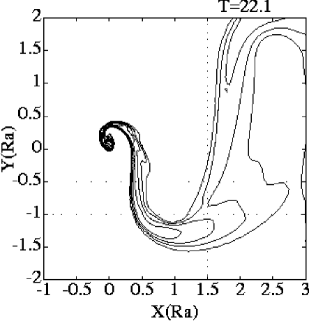
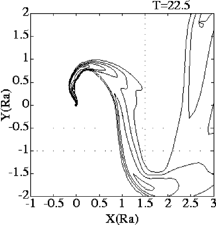
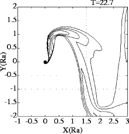
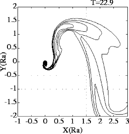
Figure 1: Density contour for the AM040_005 case, at times T=22.1, 22.3, 22.5, 22.7 and 22.9. The scale is logarithmic from 0 to 3, in steps of 0.3 .

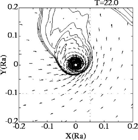
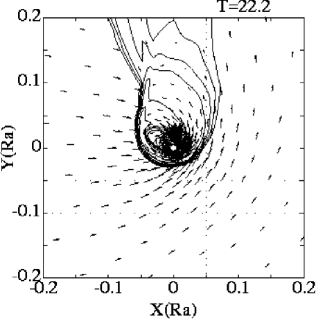
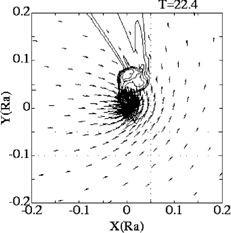
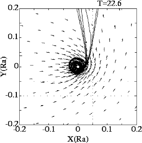
Figure 2: Density contour for the AM040_005 case, at times T=22., 22.2, 22.4, 22.6 and 22.8. The scale is logarithmic from 0 to 3, in steps of 0.6, and we have zoomed close to the star. The arrows visualize the velocity field

2.2 Initial and Boundary Conditions

Initially the whole computational field is filled with a uniform gas. The outer boundary condition is given by the analytic solution of Bisnovatyi-Kogan et al. (bis (1979)). An absorbing boundary condition, in which the density is very low and the flow velocity is zero, is used at the inner boundary.

2.3 Computational Mesh

A two dimensional cylindrical grid is used for our computations. The mesh is divided uniformly in angular zones and is divided nonuniformly in radius. The mesh size in the radial direction ($\Delta R$) changes exponentially such as, $\Delta R_{i}=\Delta R_{1}\alpha^{i-1}$.

The radius of the absorbing inner boundary ($R_{\rm min}$) is 0.01 $R_{\rm a}$ and that of the outer boundary ($R_{\rm max}$) is 10 $R_{\rm a}$. The standard grid is made of 200 mesh points in the angular direction and 140 mesh points in the radial direction. For the fine grid, these numbers are 400 and 250, respectively. The finest mesh size in the radial direction ($\Delta R_{1}$) is 0.001 $R_{\rm a}$ in both the standard and the fine grid (see Table 1).

Under astrophysical conditions, the inner boundary is usually located at the magnetopause of the compact accreting object. This radius is in general much smaller than the inner boundary of our computational domain. But even if the two values are comparable one has to realize that the numerical boundary conditions do not describe the physical situation at the magnetopause which will be much more complex. The absorbing boundary condition at the inner radius is more or less an artificial construction. In order to study the influence of $R_{\rm min}$, computations with different values of $R_{\rm min}$ were carried out.

	Angular Mesh	Radial Mesh	$R_{\rm max}/R_{\rm a}$	$R_{\rm min}/R_{\rm a}$	$\Delta R_{1}/R_{\rm a}$	$\alpha$
Standard grid	200	140	10	0.01	0.001	1.04533
Fine grid	400	250	10	0.01	0.001	1.02200

Table 1: Computational grids used in the simulations

2.4 Finite Volume Method

By applying the hydrodynamic equations in integral form to a rectangular volume constructed by mesh lines, a finite volume formulation is obtained. In order to obtain high spatial resolution, a MUSCL type approach and van Albada’s flux limiter are used. The numerical fluxes which are used by the MUSCL scheme are described in section 2.5.

Hydrodynamic and gravitational terms are integrated simultaneously. A two-step Runge-Kutta method is used for time integration. This scheme is accurate to second order in both space and time.

2.5 Simplified Flux Splitting (SFS) for Isothermal Gas

The finite volume method for solving the hydrodynamic equations takes the approximation of the flux normal to the interface which are denoted by Eqs.( 5),( 6) and ( 8).

The numerical flux in the MUSCL scheme is computed from the values defined on both sides of the cell interface by,

$$\@vec{F}=\@vec{F}(Q_{+},Q_{-})$$ (12)

where $\pm$ denote the values on the left($+$) and right($-$) side, and $m$ is the mass flux. This flux is computed by solving the Riemann initial value problem using the left and right side physical values. It is in principle possible to solve this problem exactly, but this would require a very large amount of computer time. Therefore approximate but very fast algorithms have been developed.

The way in which these are calculated is vital for the MUSCL type scheme, since it influences the computer time, robustness and accuracy. Both the robustness for strong shock waves and the accuracy for slip surfaces are necessary for this study, because of the high mach number near the object and the strong shearing in the accretion column and the disk.

Many algorithms for the numerical flux have been developed. Approximate Riemann values of the fluxes were obtained by the Roe (Roe (1981)) and (Chakravarthy & Osher Osher (1982)). Although they are exact for shocks or rarefactions of moderate strength, they give unphysical results for strong rarefactions or shocks respectively. Thus they are not robust enough for hypersonic computations like this study where very strong shocks and rarefactions are produced by the high speed flow accelerated by gravity. Flux vector splitting schemes (Steger & Warming SW (1981), van Leer VL (1982), Hänel & Schwane Haenel (1989) ) are simple and more robust, and it has been shown that they have enough accuracy for the shock tube problem or flows around airfoils. However they are not accurate for contact discontinuities such as slip surfaces, since they have excess numerical shear stress which influences the momentum transfer especially in accretion disks. Thus these existing schemes are not good enough for the supersonic accretion flow. Wada & Liou (Wada (1994)) discussed these problems in the context of to aerospace applications. Note that we consider only discontinuities in one-dimension or those aligned to grid lines in multidimensional flows. In general, discontinuities do not align to grid lines and all schemes including exact Riemann solver can not capture them exactly. Nevertheless it has been recognized that those characteristics strongly affect the accuracy.

Recently Liou & Steffen (Liou (1993)) developed an Advection Upstream Splitting Method (AUSM). Althogh the AUSM exhibits small overshoots at shocks, it is as simple and robust as flux vector splitting schemes and as accurate as the exact solver for contact discontinuities. Inspired by this work, a family of AUSM type schemes have been developed (Jounouchi et al. sfs (1993), Wada & Liou Wada (1994), Shima & Jounouchi SIMA (1997)). It has been shown that these AUSM type schemes are sufficiently simple robust and accurate.

Jounouchi et al. (sfs (1993), see also Shima & Jounouchi SIMA (1997)) developed a new AUSM type numerical flux scheme named Simplified Flux Splitting (SFS). They reduced the overshoot at the shock wave. Originally the SFS was developed for adiabatic gas, but it has been modified for an isothermal gas in this study. The SFS scheme for an isothermal gas can be written as follows.

$$\@vec{F}_{SFS}=\frac{m+|m|}{2}\@vec{\Phi}_{+}+\frac{m-|m|}{2}\@vec{\Phi}_{-}+\tilde{p}\@vec{N},$$ (13)

where $\tilde{p}$ is an average value of the pressure defined by the following relations:

$$\tilde{p}=\beta_{+}p_{+}+\beta_{-}p_{-},$$ (14)

$$\beta_{\pm}=\frac{1}{4}(2\mp\tilde{M}_{\pm})(\tilde{M}_{\pm}\pm 1)^{2},$$ (15)

$$\tilde{M}_{\pm}=min(1,max(0,M_{\pm})),$$ (16)

and

$$M_{\pm}=\frac{V_{n\pm}}{c}.$$ (17)

The mass flux $m$ is given by the flux vector splitting method as follows:

$$m=m_{+}+m_{-},$$ (18)

$$\left\{\begin{array}[]{ll}m_{\pm}=\pm 0.25\leavevmode\nobreak\ \rho_{\pm}c(M_{\pm}\pm 1)^{2}&for|M_{\pm}|\leq 1\\ m_{\pm}=0.5\leavevmode\nobreak\ \rho_{\pm}(V_{n\pm}\pm|V_{n\pm}|)&for|M_{\pm}|>1.\end{array}\right.$$ (19)

Note that the usage of the flux vector splitting does not degrade the accuracy of a contact discontinuity for isothermal gas, because at the slip surface the SFS scheme gives zero flux normal to the surface.

2.6 Angular momentum conserving scheme

Finite volume methods are usually based on the conservation laws of mass, linear momentum and total energy. Conservation of energy is not used in the present computations because the gas is isothermal. These conservation laws, of course, also imply the conservation of angular momentum for the exact solutions. The conservation of linear momentum, however, is just an approximation for the angular momentum in a discretized description. As the accuracy is at most second order in mesh size with any finite volume method, it depends on the numerical mesh.

If the accreting matter in the accretion column does not collide with itself and if it keeps some angular momentum , it will follow a Keplerian orbit and cannot accrete. Thus the formation of an accretion disk near the object directly reflects the angular momentum of the accreting matter, and it therefore depends crucially on the accuracy of the conservation of angular momentum.

The angular momentum conserving (AMC) scheme based on Eqs. (9) and (10) shows less mesh dependency than the linear momentum conserving (LMC) scheme as will be shown later. The AMC scheme can easily be obtained from the LMC scheme. In fact, the difference between the AMC and LMC computer codes is only a few lines.

2.7 Accurate local time stepping

The solutions of wind accretion are nonsteady in most cases. Therefore, the numerical scheme has to be accurate in time to capture the motion correctly. Two-step Runge-Kutta time stepping with a small Courant number (less than 0.2) was used for this purpose. Near the object, the flow has very high velocity and a fine mesh is required there for spatial resolution, thus, the size of the time step is very restricted by the Courant condition and very long computing times are required to reach physically meaningful solutions, when the usual uniform step is taken.

In order to avoid this problem, time accurate local time stepping was used in this investigation. First a global time step is defined, then the time step at each cell is divided into two if the Courant number is larger than our limit. This procedure is repeated until Courant condition is satisfied in all cells. The inner iteration is carried out in one global iteration when the local time step is smaller than the global time step The conservation laws are fulfilled by summing up the fractional fluxes correctly. A speed up by about a factor 20 was obtained by this procedure. However, over 100 hours of computer time on a 2 GFLOPS class supercomputer (Fujitsu VPP-300) were still needed for the fine mesh case.

2.8 Units

The obvious reference length is the accretion radius $R_{\rm a}$. The fluid velocity far upstream, $V_{\infty}$, is used as a reference velocity, thus the time unit is

$$T_{\rm ref}=\frac{R_{\rm a}}{V_{\infty}}.$$ (20)

The mass accretion rate is normalized by the two-dimensional Hoyle & Lyttleton rate given by

$$\dot{M}_{\rm HL}=2\rho_{\infty}V_{\infty}R_{\rm a}.$$ (21)

The angular momentum accretion rate is normalized by

$$\dot{J}_{\rm ref}=\rho_{\infty}{V_{\infty}}^{2}R^{2}_{\rm a}.$$ (22)

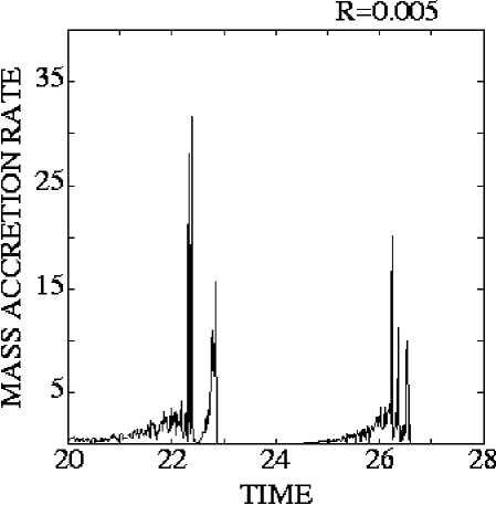
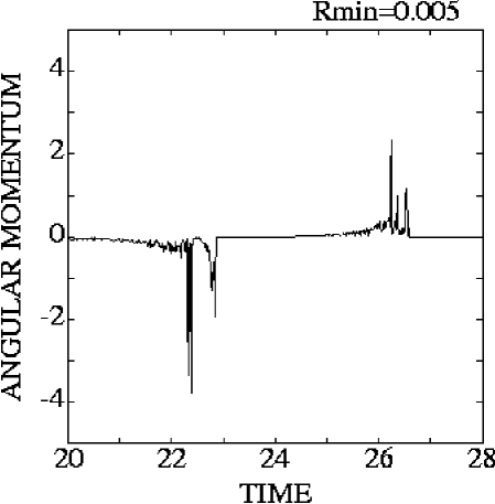
Figure 3: Time history of the mass accretion rate (left) and angular momentum accretion rate (right) for the AM040_005 case at times corresponding to Fig. 2, AMC scheme

Case	Scheme	Grid	$\cal{M}$	$R_{\rm min}$	$R_{\rm max}$	$AVE(\dot{M})$	$\dot{M}^{\prime}$	$AVE(\dot{J})$	$RMS(\dot{J})$
AF040_01	AMC	Fine	4.0	0.01	10.0	0.967	1.331	0.008	0.219
AM010_01	AMC	Standard	1.0	0.01	10.0	1.239	0.092	0.000	0.000
AM014_01	AMC	Standard	1.4	0.01	10.0	0.971	1.623	0.005	0.272
AM020_01	AMC	Standard	2.0	0.01	10.0	0.944	1.961	0.000	0.308
AM040_005	AMC	Standard	4.0	0.005	5.0	0.855	2.031	0.009	0.240
AM040_01	AMC	Standard	4.0	0.01	10.0	0.838	1.176	0.017	0.206
AM040_02	AMC	Standard	4.0	0.02	20.0	0.951	0.786	-0.008	0.201
AM080_01	AMC	Standard	8.0	0.01	10.0	1.020	1.090	0.007	0.160
AM160_01	AMC	Standard	16.0	0.01	10.0	0.982	0.938	0.010	0.125
TF040_01	LMC	Fine	4.0	0.01	10.0	1.033	3.040	0.000	0.362
LM040_005	LMC	Standard	4.0	0.005	5.0	0.420	0.395	0.0377	0.058
LM040_01	LMC	Standard	4.0	0.01	10.0	0.695	0.643	0.016	0.128
LM040_02	LMC	Standard	4.0	0.02	20.0	0.817	0.683	0.011	0.183
LM040_05	LMC	Standard	4.0	0.05	50.0	0.979	0.3355	0.0177	0.197

Table 2: Parameters and nondimensional values of each case. $\dot{M}^{\prime}$ is the root mean square of fluctuations from the averaged value of $\dot{M}$. $AVE(\dot{M})$ and $AVE(\dot{J})$ are the average of mass and momentum accretion rate respectively, and $RMS(\dot{J})$ is the root mean square of $\dot{J}$.

3 Numerical Results

3.1 Calculated Cases

The cases which we have calculated are summarized in table 2. Our main interest is in the thin accretion column of supersonic flows, thus Mach number $\cal{M}$=4 was chosen as the standard case. The results obtained with the LMC scheme exhibited more mesh dependency than those of the AMC scheme, therefore we show mainly the AMC results

3.2 Mesh Dependency of the LMC and AMC schemes

Table 2 summarizes how for both the LMC and AMC scheme the mass accretion rate, $\dot{M}$, and the RMS value of the angular momentum accretion rate, $RMS(\dot{J})$ depend on the details of the models. The mass accretion rate changes from 0.420 to 0.817 when the size of the central hole increases from 0.005 $R_{\rm a}$ to 0.02 $R_{\rm a}$ in the LMC calculations (case LM040_005, LM040_01, LM040_02). On the other hand, the mass accretion rates for the AMC cases are in the range 0.838 to 0.951.

For the LMC scheme, as the central hole becomes smaller, mass and angular momentum accretion also become smaller with the standard grid. When the central hole is large, a temporary accretion disk is formed and the averaged mass accretion rate is close to the Hoyle & Lyttleton value. But for a small central hole an almost permanent accretion disk is formed near the hole which blocks further accretion. However in the fine grid case this decrease of the mass accretion is not found and the existence of the accretion disk is temporary. On the other hand for the AMC scheme, accretion disks are always transient and accretion rates are similar.

This fact indicates that the conservation of angular momentum is very important for the accretion problem. Since the results based on the AMC scheme have less mesh dependency, they seem to be more reliable. Thus only the results from the AMC scheme will be shown in the rest of this section.

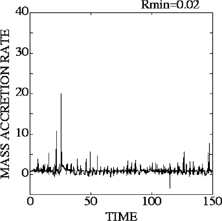
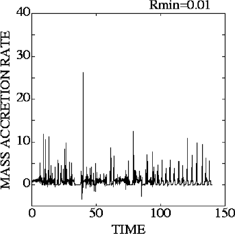
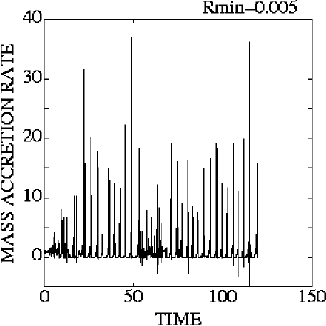
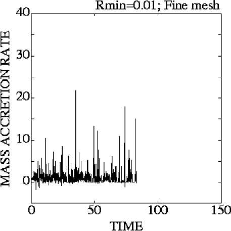
Figure 4: Time history of the mass accretion rate. $\cal{M}$=4.0; $R_{\rm min}$=0.02, .01, .005 and .01 fine grid, AMC scheme

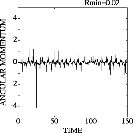
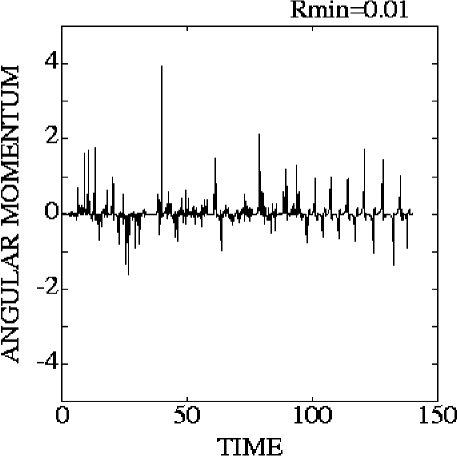
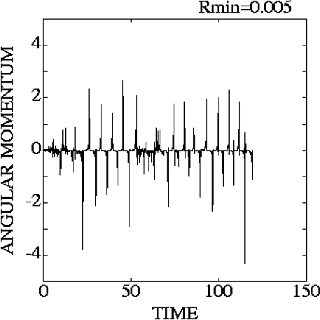
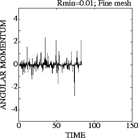
Figure 5: Time history of the angular momentum accretion rate. $\cal{M}$=4.0; $R_{\rm min}$=0.02, .01, .005 and .01 fine grid, AMC scheme

3.3 Occurrence of Oscillations and Formation of Accretion Disks

The accretion column of the supersonic accretion flow is narrow and large oscillations are found. In Figure 1, the typical sequence of the swinging of the accretion column of case AM040005 is shown. The oscillating accretion column swings over 180 degrees. This oscillation is similar to that shown in the computation of Boffin and Anzer (bof (1994)), but there is also an accretion disk in our computation. The radius of the accretion disk is about 0.1 $R_{\rm a}$.

Enlarged views are shown in Fig. 2. The formation and destruction of the accretion disk is clearly seen in these figures. An anti-clockwise rotating accretion disk is formed at T=22. The accreting matter falls from the upper-left direction through the accretion column, thus this matter has anti-clockwise angular momentum and it accelerates the disk. Then the column is pushed backward by accreting matter from upstream. When the column moves behind the object, the accreting matter has clockwise angular momentum (T=22.2). This matter collides with the disk and destroys the disk (T=22.4). Then a clockwise rotating disk is formed (T=22.6 and following). As shown in Fig. 3, mass and angular momentum is accreted when the disk collapses.

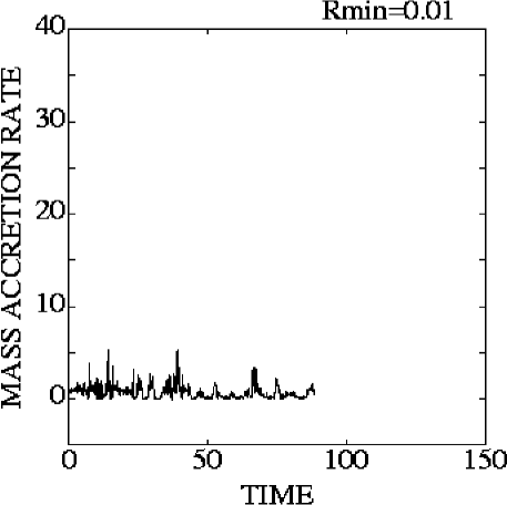
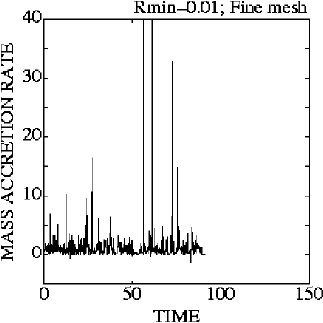
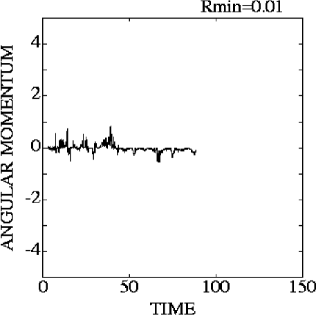
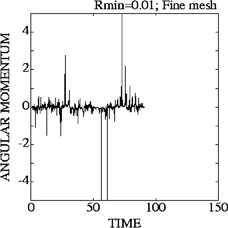
Figure 6: Time history of the mass accretion rate (upper frames) and angular momentum accretion rate (lower frames). $\cal{M}$=4.0 $R_{\rm min}=0.01$. The results from the standard grid (left) and from the fine grid (right) are shown, LMC scheme

The averaged mass accretion rate of this case is 0.855, but the instantaneous rate is over 10 times larger than the Hoyle & Lyttleton estimate. The averaged momentum accretion is almost zero. However, a fair amount of instantaneous angular momentum accretion with altering direction is also found. This can be understood as follows: the symmetric accretion column cannot have angular momentum, but the portions of an asymmetric accretion column can have angular momentum. When the positive angular momentum portion falls downward, a positive accretion disk is formed. This accretion disk loses its angular momentum and accretes onto the object, when it collides with the following portion which has negative angular momentum.

3.4 History of Mass Accretion Rate and Angular Momentum Accretion

The histories of mass accretion and angular momentum accretion of representative cases from the AMC scheme are shown in Fig. 4 and 5. Those from the LMC scheme are shown in Fig. 6.

3.4.1 Effects of $R_{\rm min}$ and Mesh size

The histories of accretion rates for $\cal{M}$=4.0 from the AMC scheme with different $R_{\rm min}$ and mesh size are shown in Figs. 4 and 5. As seen in those figures, the fluctuations of the accretion rate become bigger with smaller $R_{\rm min}$.

Figure 7: Mach number dependency of characteristic values for the AMC case with standard grid

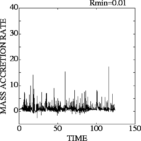
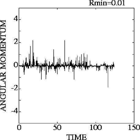
Figure 8: Time history of the mass accretion rate (left) and of the angular momentum accretion rate (right). $\cal{M}$=8.0 $R_{\rm min=0.01}$

We can see from table 2 and Fig. 4 that the mean values of the mass accretion rate are quite similar for different values of $R_{min}$, whereas the peak amplitudes of $\dot{M}$ increase with decreasing $R_{min}$. This then implies that the accretion bursts are correspondingly shorter for smaller values of $R_{min}$. Although the results for the fine grid (Fig. 4 & 5) have fluctuations of higher frequency and are more chaotic, they are generally similar to those for the standard grid. The similarity is also clearly seen in Table 2. All values except $\dot{M}^{\prime}$ are similar for different $R_{\rm min}$. The sequences of the oscillations are also similar. The difference in $\dot{M}^{\prime}$ can be explained by the mechanism of the accretion disk destruction. The orbits of the anti-clockwise rotating accretion disk in Fig. 2 are almost circular, but become elliptical when the accreting mater which has clockwise angular momentum interacts with matter of the anti-clockwise rotating disk (T=22.2 in Fig. 2). The matter is taken away from the computational space when its elliptic orbit touches the central hole. Thus, the bigger central hole absorbs the matter over a longer period than the smaller hole. Therefore the fluctuation of mass accretion becomes larger for a smaller hole.

On the other hand, the LMC scheme shows a different $R_{\rm min}$ dependence. For the standard grid, the mass accretion rate becomes smaller as $R_{\rm min}$ decreases, as can be seen from the average values of $\dot{M}$ which are given in table 2.. Because an almost permanent accretion disk is formed it blocks further accretion. But this permanent accretion disk is not found for the fine grid. In this case the accretion rates show large fluctuations. The conservation of angular momentum is only achieved to second order accuraey in the LMC scheme. Thus, we believe that the standard grid is not fine enough for the LMC scheme to capture the accretion disk formation.

3.4.2 Effects of the Mach Number

If the Mach number of the uniform flow is 1, the flow is perfectly steady, but for larger Mach number it is always non-steady. Note that the case of $\cal{M}$=1.4 is also non-steady and shows small fluctuations from the beginning. However, non-steadiness with large amplitudes occurs only after 40 time units. The Mach number dependence of the averaged mass accretion rate, the fluctuation of the mass accretion rate and the fluctuation of the angular momentum accretion rate are summarized in Fig. 7. These are the results from the AMC scheme with the standard grid.

As shown in Fig. 7 the amplitude of the oscillations is largest when the Mach number is 2, and the fluctuations become smaller as the Mach number becomes greater than 4. This is also shown in the history of the mass and angular momentum accretion of the Mach 8 case (case AM080_01) in Fig. 8.

As the Mach number increases, the amplitudes of the accretion column oscillation become smaller. This behavior is clearly shown in the time averaged density contours of Fig. 9. In the time averaged solution, the wiggles of the accretion column are smeared out and the high density regions around the accreting object are seen. The high density regions are concentrated in a narrow cone in the high Mach number cases (see the ${\cal{M}}$=8 case in Fig. 9). It is interesting that the transient accretion disks are also seen as high density regions in the averaged solutions and that averaged accretion columns look like bow shocks.

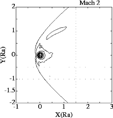
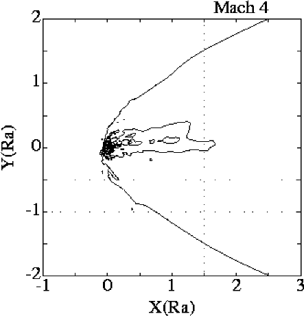
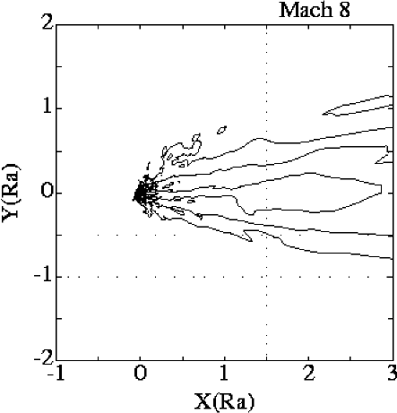
Figure 9: Time averaged density contour. Rmin=0.01, $\cal{M}$=2,4 and 8. The contours are logarithmically spaced between 0 and 3, in steps of 0.3

4 Summary and discussion

Two dimensional planar wind accretion flows of a supersonic isothermal gas were analyzed numerically. The computational efficiency was improved as compared to earlier calculations by using an accurate local time stepping and a new type of upwind scheme.

Comparing our new results with earlier calculations one realises that 2D flows with $\gamma$ close to unity have so far not been studied very systematically. Matsuda et al. (1992) presented one case with $\gamma=1.05$ and one with $\gamma=1.005$. Their resolution near the central object was much coarser than our resolution. They had also obtained flip-flop configurations, but the instability took much longer to develop. Their amplitudes were smaller and the widths of the accretion columns considerably larger. Boffin and Anzer (1994) also calculated one model with $\gamma=1.1$ which has a narrow oscillating accretion column, but again a low amplitude. 3D flows with $\gamma=1.01$ have been systematically studied by Ruffert ( 1996). In these flows the accretion regions are always much wider and do not show the systematic oscillations of entire accretion region, although the accretion itself is non-steady. There differences between 3D and 2D flows are quite general and independent of the value of $\gamma$.

We also have developed a numerical scheme which exactly conserves angular momentum (AMC scheme) and compared its performance to the earlier linear momentum conserving (LMC) scheme. We found that the results obtained with our LMC scheme depend very strongly on the resolution of the grid used, whereas the AMC scheme gives almost no difference for the two types of resolution considered here. Therefore we feel that the AMC calculations are much more reliable and all the results presented in the previous section are based on this scheme. The fact that our AMC and LMC results differ by large amounts suggests to us that many of the earlier calculations which basically conserve linear momentum should be taken with caution. This will be particularly important for the temporal behavior of the accretion of angular momentum $\dot{J}$ (t).

Our calculations of supersonic flows show that in all cases the accretion of both mass and angular momentum is very erratic. It occurs in very short intervals and at extremely high rates. This behavior can be explained by the formation of Keplerian disks near the inner boundary. If the specific angular momentum of the infalling material is larger than that of the Kepler orbit at the innermost radius then this material cannot accrete.

If such high angular momentum material is flowing in long enough, a disk will form which blocks further accretion very efficiently. Material with very low angular momentum or with opposite rotation falling in during a subsequent phase interacts with the disk and can destroy it. This will lead to a burst of the accreted mass and angular momentum. After such a burst the process can be repeated and a new disk will form. Our calculations indicate that reversals of the disk rotation are quite common.

For the modeling of X-ray binaries fed by wind accretion the fluctuations of $\dot{J}$ are of major importance. They can be brought into relation with the observed spin-up and spin-down of these X-ray pulsars; see Anzer & Börner (anz (1995)). In their investigation they showed that the random fluctuations calculated by Ruffert (1994a ) for 3d models were by a factor $\approx 10$ too low in order to explain the pulse period variations observed in the source Vela X-1. However our new calculations give variations of $\dot{J}$ which are substantially larger than those found by Ruffert. We have obtained typical values of RMS $(\dot{J})$ of the order of 0.2 in our dimensionless units (see Table 2). This result can also be formulated as:

$$RMS(\dot{J}) = 0.2\leavevmode\nobreak\ \rho_{\infty}\leavevmode\nobreak\ {v^{2}_{\infty}}\leavevmode\nobreak\ R_{\rm a}^{2}$$

$$= 0.1\leavevmode\nobreak\ \dot{M}_{HL}\leavevmode\nobreak\ {v_{\infty}}\leavevmode\nobreak\ R_{\rm a}$$

$$\approx 0.1\leavevmode\nobreak\ {v_{\infty}}\leavevmode\nobreak\ R_{\rm a}$$

since $\dot{M}$ is typically of the order unity. On the other hand Ruffert (Rufd (1996)) gives RMS(j)=0.01${v_{\infty}}R_{\rm a}$ for $\gamma=1.01$ and RMS(j) = 0.03${v_{\infty}}R_{\rm a}$ for $\gamma=5/3$. Taking into account that RMS($\dot{J}$)=RMS ($\overline{\dot{M}}$j) and $\overline{\dot{M}}$ $\approx 1$ we have RMS ($\dot{J}$) = (0.01-0.03)${v_{\infty}}R_{\rm a}$. Therefore our values for the fluctuations area factor 3 to 10 larger than those of Ruffert’s 3D calculations. Therefore on the basis of our calculations one might conclude that the observed period fluctuations could in principle, be caused by random fluctuations of $\dot{J}$. But the amplitudes are only marginally large enough and any slight reduction of the efficency would rule out this interpretation. There is in particular the aspect that our calculations are two–dimensional whereas the real flows are three–dimensional and the difference in amplitudes between 2D and 3D flows could be sufficiently large to make the described interpretation invalid. To really answer this question requires full 3D computations, taking angular momentum conservation into account.

- (1) Anzer, U., Börner, G., 1995, A&A, 299, 62
- (2) Benensohn, J.S., Lamb, D.Q., Taam, R.E., 1997, ApJ, 478, 123
- (3) Bisnovatyi-Kogan, G.S., Kazhdan, Ya.M., Klypin, A.A., Lustkii, A.E., Shakura, N.I., 1979, SvA, 23, 201
- (4) Boffin, H.M.J., Anzer, U., 1994, A&A, 284, 1026
- (5) Bondi, H., 1952, MNRAS, 112, 195
- (6) Bondi, H., Hoyle, F., 1944, MNRAS, 104, 273
- (7) Chakravarthy, S.R., Osher, S., 1982, AIAA Paper 82-0975
- (8) Fryxell, B.A., Taam, R.E., 1988, ApJ, 335, 862
- (9) Hänel, D., Schwane, R., AIAA Paper 89-0274, 1989
- (10) Ho, C., Taam, R.E., Fryxell, B.A., Matsuda, T., Koide, H., Shima, E., 1989, MNRAS, 238, 1447
- (11) Hoyle, F., Lyttleton, R.A., 1939, Proc.Cam.Phil.Soc., 35,405
- (12) Hunt, R., 1971, MNRAS, 154, 141
- (13) Hunt, R., 1979, MNRAS, 188, 83
- (14) Ishii, T., Matsuda, T., Shima, E., Livio, M., Anzer, U., Börner, G., 1993, ApJ, 404, 706
- (15) Jounouchi, T., Kitagawa, I., Sakasita, S., Yasuhara, M., 1993, Proceedings of 7th CFD Symposium, in Japanese
- (16) Koide, H., Matsuda, T., Shima, E., 1991, MNRAS, 252, 473
- (17) Liou, M.S., Steffen, C.J., 1993, J. Comp. Phys., 107, 23
- (18) Livio, M., Soker, N., Matsuda, T., Anzer, U., 1991, MNRAS, 253, 633
- (19) Matsuda, T., Inoue, M., Sawada, K., 1987, MNRAS, 226, 785
- (20) Matsuda, T., Sekino, N., Sawada, K., Shima, E., Livio, M., Anzer, U., Böner, G., 1991, A&A, 248, 301
- (21) Matsuda, T., Ishii, T., Sekino, N., Sawada, K., Shima, E., Livio, M., Anzer, U., 1992, MNRAS 255, 183.
- (22) Roe, P.L, 1981, J.Comp.Phys., 43, 357
- (23) Ruffert, M., 1994a, ApJ, 427, 342
- (24) Ruffert, M., 1994b, A&AS, 106, 505
- (25) Ruffert, M., 1995, A&AS, 113, 133
- (26) Ruffert, M., 1996, A&A, 311, 817
- (27) Ruffert, M., Arnett, D., 1994, ApJ, 427, 351
- (28) Sawada, K., Matsuda, T., Anzer U., Börner, G., Livio, M., 1989, A&A, 231, 263
- (29) Shima, E. , Jounouchi, T., 1997, NAL-SP34,Proceedings of 14th NAL symposium on Aircraft Computational Aerodynamics, p.7
- (30) Shima, E., Matsuda, T., Takeda, H., Sawada, K., 1985, MNRAS 217, 367
- (31) Steger, J.L., Warming, R.F., 1981, J.Comp.Phys., 40, 263
- (32) Taam, R.E., Fryxell, B.A., 1988, ApJ, 327, L73
- (33) van Leer, B., 1982, Lecture Note in Physics, 170, 507
- (34) Wada, Y. , Liou, M.S., 1994, AIAA Paper 94-0083