The Cosmic Microwave Background and Observational Convergence in the ${\Omega_{m}}-{{\Omega_{\Lambda}}}$ Plane

Abstract

I use the most recent cosmic microwave background (CMB) anisotropy measurements to constrain the leading cold dark matter models in the ${\Omega_{m}}-{{\Omega_{\Lambda}}}$ plane. A narrow triangular region is preferred. This triangle is elongated in such a way that its intersection with even conservative versions of recent supernovae, cluster mass-to-light ratios and double radio source constraints, is small and provides the current best limits in the ${\Omega_{m}}-{{\Omega_{\Lambda}}}$ plane: ${{\Omega_{\Lambda}}}=0.62\pm 0.16$ and ${\Omega_{m}}=0.24\pm 0.10$. This complementarity between CMB and other observations rules out ${{\Omega_{\Lambda}}}=0$ models at more than the $99\%$ confidence level.

1 INTRODUCTION

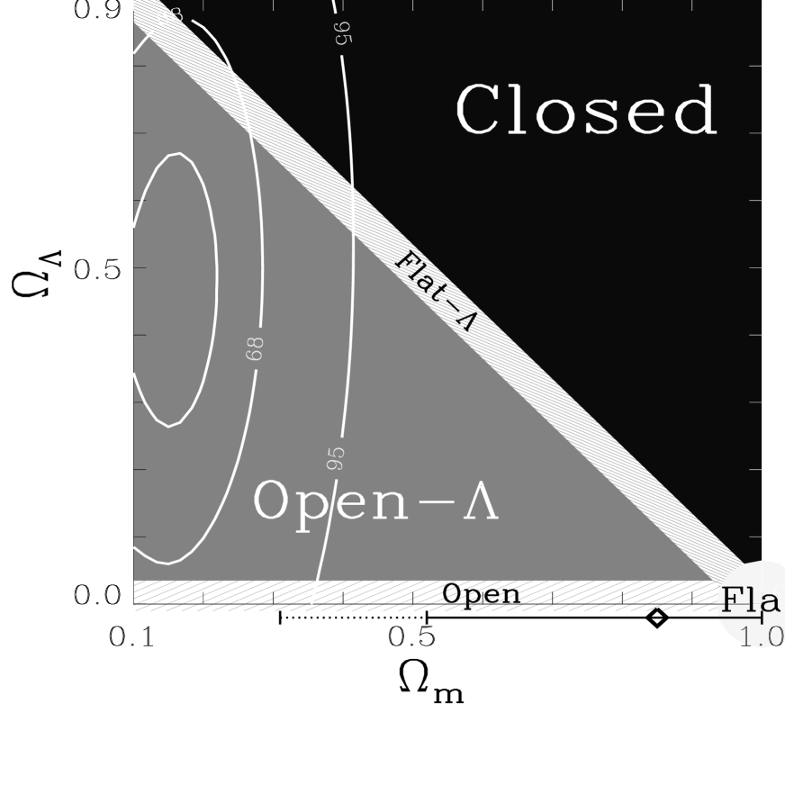
Figure 1: Overview of cold dark matter (CDM) models in the ${\Omega_{m}}-{{\Omega_{\Lambda}}}$ plane. This parameter space includes the popular cosmological candidates: flat, flat-$\Lambda$ and open models as well as the less popular open$-\Lambda$ models. Closed models (upper right triangle) are not considered here. The white contours indicate the region favored by the joint likelihood of constraints from recent supernovae, cluster mass-to-light ratios, and double radio sources. They are approximate $38.3\%,68.3\%$ and $95.4\%$ confidence regions (see Table 1 and Section 4). In open models (${{\Omega_{\Lambda}}}=0$) there is a significant inconsistency between CMB results and these other observations. Previously reported constraints from the CMB in open models are indicated just below the ${\Omega_{m}}$ axis: ${\Omega_{m}}=0.85$ with a $68.3\%$ lower limit of $0.53$ and a $99.9\%$ lower limit of $0.31$ (Lineweaver & Barbosa 1998b).

The main goal of CMB measurements and the two new satellite missions MAP and Planck Surveyor is to determine a host of cosmological parameters at the unprecedented accuracy of a few percent (Jungmann et al. 1996, Zaldarriaga et al. 1997, Bond et al. 1997). As part of this goal it is important to keep track of what can already be determined from the CMB without conditioning on certain families of models or on certain values of parameters within these families. In this Letter, the analysis of CMB anisotropy measurements is expanded to include the most popular families of cold dark matter (CDM) models such as flat, flat-$\Lambda$ and open models, as well as the less popular open$-\Lambda$ models. Figure 1 presents an overview of this parameter space. Open-$\Lambda$ models are considered here because they subsume all of the above models and thus provide a parameter space in which the most popular models can be directly compared.

The popularity of non-zero ${{\Omega_{\Lambda}}}$ models has waxed and waned over the years; for excellent reviews see Felten & Isaacman (1986) and Carroll et al. (1992). ${{\Omega_{\Lambda}}}$ was introduced by Einstein (1917) to solve the discrepancy between an apparently static universe and the dynamic cosmology of general relativity. Since this inauspicious beginning ${{\Omega_{\Lambda}}}$ has been invoked many times and seems to be a surprisingly multi-purpose cure-all for theory-observation mismatches. Several recent papers (Turner 1991, Ostriker & Steinhardt 1995, Roos & Harun-or-Rachid 1998), have pointed out the effectiveness of ${{\Omega_{\Lambda}}}$ in resolving apparent conflicts between various observational constraints. Recently, ${{\Omega_{\Lambda}}}$ has been invoked to solve the discrepancy between globular cluster ages and the age of the Universe inferred from measurements of Hubble’s constant.

Recent supernovae results in ${{\Omega_{\Lambda}}}=0$ models yield ${\Omega_{m}}$ values so low that they are unphysical: ${\Omega_{m}}=-0.4\pm 0.5$ (see column 2 of Table 1, error bars and limits in this Letter are $68\%$ confidence levels unless stated otherwise). Not only are they unphysically low but the highest ${\Omega_{m}}$ values allowed by the error bars are in strong disagreement with the high values of ${\Omega_{m}}$ preferred by the CMB in these same models (Lineweaver 1998). In Lineweaver & Barbosa (1998b) we report a 99.9% confidence lower limit of ${\Omega_{m}}>0.31$ (see Figure 1). This supernovae/CMB inconsistency is strong motivation to use CMB data to explore a larger parameter space which includes ${{\Omega_{\Lambda}}}$. If the inconsistency is caused by the incorrect assumption that ${{\Omega_{\Lambda}}}=0$, then such an analysis will show it. The result of the analyis presented here is that ${{\Omega_{\Lambda}}}>0$ can resolve this inconsistency.

Testing large parameter spaces is important to minimize the model dependence of the results. For example, in Lineweaver & Barbosa (1998a) the CMB data favored ${h}=0.30^{+0.18}_{-0.07}$ (if ${\Omega_{m}}=1$, if ${{\Omega_{\Lambda}}}=0$ and if all the other assumptions made are valid). In Lineweaver & Barbosa (1998b), hereafter LB98b, we dropped the ${\Omega_{m}}=1$ assumption and still found low ${h}$ values (${h}=0.40$ but with large error bars: $0.26<{h}<0.97$) and ${\Omega_{m}}>0.57$. Thus the CMB data prefer high ${\Omega_{m}}$ values (if ${{\Omega_{\Lambda}}}=0$). These may be big if ’s. The purpose of this paper is to make these if ’s smaller by exploring a still larger region of parameter space.

Other workers have used CMB observations to constrain cosmological parameters in CDM models ( e.g. Bond & Jaffe 1997, deBernardis et al. 1997, Ratra et al. 1997, Hancock et al. 1998, Lesgourgues et al. 1998, Bartlett et al. 1998, Webster et al. 1998, White 1998). The previous work most similar to this Letter is White (1998). White (1998) combined supernovae results with the Hancock et al. (1998) estimate of the position in $\ell-$space of the peak in the CMB power spectrum. In Section 5, I compare my results to White (1998) and other work.

2 Method

I use $\chi^{2}$ minimization to identify the best fit and $\Delta\chi^{2}=[1,4,9,16]$ to identify $[68.3\%,95.4\%,99.7\%,99.9\%]$ confidence regions around the minima. The $\chi^{2}$ computation is

$$\chi^{2}({\mathbf{\theta}})=\sum_{i}\frac{(model({\mathbf{\theta}})-data_{i})^{2}}{\sigma_{i}^{2}},$$ (1)

where ${\mathbf{\theta}}=[{{\Omega_{\Lambda}}},{\Omega_{m}},{h},{\Omega_{b}h^{2}},{n},{Q_{10}}]$ which are, respectively, the cosmological constant, the matter density, Hubble’s constant, the baryonic density, the primordial power spectrum index and the primordial power spectrum amplitude at $\ell=10$. ${{\Omega_{\Lambda}}}$ and ${\Omega_{m}}$ are normalized to the critical density (${{\Omega_{\Lambda}}}={\Lambda}/3H_{o}^{2}$, ${\Omega_{m}}=\rho_{m}/\rho_{crit}$) and ${h}$ is the dimensionless Hubble constant normalized at $100\>km\;s^{-1}\;Mpc^{-1}$. The following ranges for these parameters were used: $0\leq{{\Omega_{\Lambda}}}\leq 0.9,\>0.1\leq{\Omega_{m}}\leq 1.0,\>0.15\leq{h}\leq 1.00,\>0.005\leq{\Omega_{b}h^{2}}\leq 0.030,\>0.58\leq{n}\leq 1.42,14.0\>\mu$K $\leq{Q_{10}}\leq 23\;\mu$K with respective stepsizes $0.05,0.05,0.05,0.005,0.03,0.5$. Although I am exploring a 6 dimensional parameter space I limit the discussion in this Letter to the ${\Omega_{m}}-{{\Omega_{\Lambda}}}$ plane. A $\chi^{2}$ value is calculated for all points in the ranges above, consistent with the condition ${\Omega_{b}}\leq{\Omega_{m}}$. All 6 parameters are free to take on any value which minimizes the $\chi^{2}$. See §2 of Lineweaver et al. (1997) and §2 of LB98b for more details of the method. Compared to LB98b the improvements here are: 1) inclusion of ${{\Omega_{\Lambda}}}$ as an extra dimension of parameter space ( not just flat$-\Lambda$), 2) new and updated CMB data points, 3) a larger range and higher resolution in the ${\Omega_{b}h^{2}}$ dimension, 4) the weak dependence of the helium fraction $Y_{He}$ on ${\Omega_{b}h^{2}}$ is included (Sarkar 1996, Hogan 1996). Previously we had just set $Y_{He}=0.24$ for all values of ${\Omega_{b}h^{2}}$.

The models in Eq. (1) were computed with CMBFAST (Seljak & Zaldarriaga 1996). The sum on $i$ in Eq. (1) is over 35 independent CMB anisotropy measurements. These data points are given in Table 1 of LB98b with the following updates: two new points from Femenía et al. (1998), updated values from Baker (1998) and Leitch (1998) to conform to the final published results and improved estimates of the error bars on the earlier MSAM results. The previous 5 MAX points have been combined into one point (Tanaka 1997) and I use the uncorrelated DMR points reported in Tegmark & Hamilton (1997). I also now include the data point from Picirillo & Calisse (1993). In this analysis I use the Leitch (1998) recalibration of the Saskatoon measurements (Netterfield et al. 1997) which involves a $5\%$ increase in amplitude with a $4\%$ dispersion about the new central values (see Section 2.3 of LB98b).

I have compared the results from LB98b with results from this updated data set in open models (${{\Omega_{\Lambda}}}=0$). The difference is small. LB98b reported $0.26<{h}<0.97$ and ${\Omega_{m}}>0.53$, (${\Omega_{m}}>0.31$ at 99.9% confidence level) with central values of ${h}=0.40$ and ${\Omega_{m}}=0.85$. The analogous result with the new data set is $0.30<{h}<0.98$ and ${\Omega_{m}}>0.57$ (${\Omega_{m}}>0.34$ at 99.9% confidence level) with central values ${h}=0.55$ and ${\Omega_{m}}=0.75$.

3 CMB Results

The main result of the CMB analysis is shown in Fig. 2. The CMB data prefer the narrow hashed region (68.3% confidence level) enclosed by approximate 95.4%, 99.7% and 99.9% contours. The ‘X’ marks the best fit: $({\Omega_{m}},{{\Omega_{\Lambda}}})=(0.45,0.35)$. The minimum $\chi^{2}$ value is 22.1. With normally distributed errors, the probability of obtaining a $\chi^{2}$ this low or lower is $22.3\%$.

Since we have not considered closed models, the 68.3% confidence region is cut off by the ${\Omega_{m}}+{{\Omega_{\Lambda}}}=1$ limit. However the $\chi^{2}$ values along this cutoff are very close to the 68.3% confidence level. Thus when the entire square is explored one should expect the 68.3% confidence region to widen only for ${\Omega_{m}}\mbox{$\>\stackrel{{\scriptstyle>}}{{{}_{\sim}}}\>$}0.5$ and only by a narrow strip approximately parallel to the ${\Omega_{m}}+{{\Omega_{\Lambda}}}=1$ line. If one restricts the analysis to flat-${\Lambda}$ models, the best-fit is ${{\Omega_{\Lambda}}}=0.1$ with an upper limit ${{\Omega_{\Lambda}}}<0.61$.

This analysis also yields new constraints on the power spectral index and on the power spectrum normalization. At the $\chi^{2}$ minimum ${n}=1.06^{+0.12}_{-0.18}$ and ${Q_{10}}=18\pm 1\;\mu$K. The best-fit Hubble’s constant is $h=0.75$ but with a large 68.4% confidence range $0.35<{h}<0.98$. Thus ${h}$ is not very usefully constrained by the CMB alone. The $\chi^{2}$ minimum is obtained at the maximum value considered for the baryonic density: ${\Omega_{b}h^{2}}=0.030$ with a 68.4% lower limit of $0.025$. Thus the CMB prefers high ${\Omega_{b}h^{2}}$ values.

4 Combining Constraints

Current observational constraints from supernovae, cluster mass-to-light ratios and double radio sources in the ${\Omega_{m}}-{{\Omega_{\Lambda}}}$ plane are given in Table 1. To approximate the region of the ${\Omega_{m}}-{{\Omega_{\Lambda}}}$ plane favored by non-CMB observations, I form likelihoods from the limits in Table 1 and from published contours (e.g. Riess et al. 1998, Fig. 6, Carlberg et al. 1998, Fig. 1, Daly et al. 1998, Fig. 1). I then form joint likelihoods ${\mathcal{L}}_{non-CMB}={\mathcal{L}}_{SN}\times{\mathcal{L}}_{Clusters}\times{\mathcal{L}}_{radio}$, where all terms are functions of ${\Omega_{m}}$ and ${{\Omega_{\Lambda}}}$. The CMB results are combined with the non-CMB results in the same way: ${\mathcal{L}}_{tot}={\mathcal{L}}_{CMB}\times{\mathcal{L}}_{non-CMB}$.

There are a variety of ways in which the limits can be selected and combined. My strategy is to be reasonably conservative by trying not to over-constrain parameter space. Practically this means using contours large enough to include possible systematic errors. For example, two independent supernovae groups are in the process of taking data and refining their analysis and calibration techniques. Table 1 lists their current limits (ref. 3 & 6) which are consistent. I combine each supernovae result separately with the CMB constraints and list the result in the row marked ‘+ CMB’ directly under the supernovae result. However, the main result I quote in the abstract (last row of Table 1) comes from using the least-constraining of the two (ref. 3) in the conservative combination of non-CMB constraints, i.e., ${\mathcal{L}}_{tot}={\mathcal{L}}_{CMB}\times{\mathcal{L}}_{non-CMB(conservative)}$. Figure 3 shows each of the three terms in this equation.

I apply the same strategy with the Carlberg et al. (1997, 1998) cluster mass-to-light ratios. They report 30% errors in their ${\Omega_{m}}$ result but also cite a “worst case” of a 73% error if all the systematic errors conspire and add linearly. In Table 1, I give the result of combining the 30% and 73% versions separately with the CMB constraints. However, I use the 73% error in the conservative combination of non-CMB constraints. Thus the ${{\Omega_{\Lambda}}}=0.62\pm 0.16$ and ${\Omega_{m}}=0.24\pm 0.10$ quoted in the abstract are conservative in the sense that the error bars from the SNIa and cluster mass-to-light ratios are “worst case” error bars. A summary of the systematic error analysis of the cluster mass-to-light ratios result is given in Section 9 of Carlberg et al. (1997) and of the supernovae results in Section 5 of Riess et al. (1998).

The conservative result we quote is robust in the sense that when any one of these non-CMB constraints is combined with the CMB constraints, similar results are obtained: ${{\Omega_{\Lambda}}}=0$ is more than the $95.4\%$ confidence level away from the best-fit. Systematic errors may compromise one or the other of the observations but are less likely to bias all of the observations in the same way.

Those confident in the Riess et al. (1998) and the Carlberg et al. (1997, 1998) results should quote the extremely tight limits labelled ‘optimistic’ in the penultimate row of Table 1: ${\Omega_{m}}=0.18\pm 0.04$ and ${{\Omega_{\Lambda}}}=0.71^{+0.07}_{-0.08}$. In this small region of the ${\Omega_{m}}-{{\Omega_{\Lambda}}}$ plane the CMB data prefer ${h}=0.80\pm 0.10$, ${Q_{10}}=18\pm 0.5\>\mu$K, ${n}=1.0\pm 0.1$ and ${\Omega_{b}h^{2}}\sim 0.025$.

Table 1: Non-CMB and Non-CMB + CMB Constraints on ${{\Omega_{\Lambda}}}$ and ${\Omega_{m}}$

Reference) Method	${{\Omega_{\Lambda}}}=0$	${\Omega_{m}}+{{\Omega_{\Lambda}}}=1$		${\Omega_{m}}+{{\Omega_{\Lambda}}}\leq 1$
	${\Omega_{m}}$	${\Omega_{m}}$	${{\Omega_{\Lambda}}}$	${\Omega_{m}}$	${{\Omega_{\Lambda}}}$
1) SNIa	$0.88^{+0.69}_{-0.60}$	$0.94^{+0.34}_{-0.28}$	$0.06^{+0.28}_{-0.34}$
2) SNIa	$-0.2\pm 0.4$	$0.6\pm 0.2$	$0.4\pm 0.2$
3) SNIa	$-0.4\pm 0.51^{a}$	$0.27\pm 0.3^{b}$	$0.73\pm 0.3$
3) SNIa + CMB				$0.33^{+0.15}_{-0.18}$	$0.52^{+0.25}_{-0.22}$
4) SNIa	$-0.1\pm 0.5$	$0.65\pm 0.3^{c}$	$0.35\pm 0.3$
5) SNIa	$-0.2^{+1.0}_{-0.8}$	$0.4^{+0.5}_{-0.4}$	$0.6^{+0.4}_{-0.5}$
6) SNIa	$-0.35\pm 0.18$	$0.24^{+0.17}_{-0.10}{}^{d}$	$0.76^{+0.10}_{-0.17}$
6) SNIa + CMB				$0.26^{+0.09}_{-0.11}$	$0.63^{+0.14}_{-0.15}$
7) Cluster M/L	$0.19\pm 0.14^{e}$
7) Cluster M/L + CMB				$0.24\pm 0.10$	$0.62^{+0.17}_{-0.19}$
7) Cluster M/L	$0.19\pm 0.06^{f}$
7) Cluster M/L + CMB				$0.17^{+0.04}_{-0.03}$	$0.73^{+0.07}_{-0.08}$
8) Double Radio Sources	$-0.1^{+0.5}_{-0.4}$	$0.2^{+0.3}_{-0.2}$	$0.8^{+0.2}_{-0.3}$
8) Double Radio Sources + CMB				$0.33^{+0.16}_{-0.18}$	$0.52\pm 0.25$
Non-CMB(optimistic)g				$0.16\pm 0.05$	$0.57\pm 0.25$
Non-CMB(conservative)h				$0.15\pm 0.13$	$0.46^{+0.41}_{-0.41}$
Non-CMB(optimistic) + CMBg				$0.18\pm 0.04$	$0.71^{+0.07}_{-0.08}$
Non-CMB(conservative) + CMBh				${\mathbf{0}.24\pm 0.10}$	${\mathbf{0}.62\pm 0.16}$

^a $-0.4\pm 0.1\pm 0.5$ (statistical and systematic errors respectively) I have added the statistical and systematic errors in quadrature
^b $0.27\pm 0.06\pm 0.3$ (statistical and systematic errors respectively) I have added the statistical and systematic errors in quadrature
^c as quoted in Riess et al. 1998
^d Riess et al. (1998), Figure 6 (‘MLCS method’ + ‘snapshot method’) using either the solid or dotted contours whichever is larger (corresponding respectively to the analysis with and without SN1997ck).
^e “worst case” result with $73\%$ errors (Carlberg et al. 1997, p 473)
^f 30% error cited as the main result
^g optimistic combined constraints using SNIa results from ref. 6) (rather than ref. 3) and using the 30% error bars (rather than the 73% error bars) from Carlberg et al. (1997)
^h conservative combined constraints using SNIa results from ref. 3) (rather than ref. 6) and using the 73% error bars (rather than the 30% error bars) from Carlberg et al. (1997)

1) Perlmutter et al. (1997), 2) Perlmutter et al. (1998), 3) Perlmutter private communication (1998), 4) Garnavich et al. (1998), 5) Schmidt et al. (1998), 6) Riess et al. (1998), 7) Carlberg et al. (1997) and Carlberg et al. (1998), 8) Daly et al. (1998)

It would be useful to add constraints on ${{\Omega_{\Lambda}}}$ from lensing. Although Kochanek (1996) and Falco, Kochanek & Muñoz (1998) report ${{\Omega_{\Lambda}}}\mbox{$\>\stackrel{{\scriptstyle<}}{{{}_{\sim}}}\>$}0.7$, the lensing estimates from Chiba & Yoshii (1997) (${{\Omega_{\Lambda}}}\sim 0.8$) and Fort et al. (1997) (${{\Omega_{\Lambda}}}\sim 0.6$) are in agreement with the result found here. Thus lensing limits on ${{\Omega_{\Lambda}}}$ still seem too uncertain to add much to the analysis. However, when I fold ${{\Omega_{\Lambda}}}<0.7$ into the analysis the result for ${{\Omega_{\Lambda}}}$ comes down less than $0.5\;\sigma$.

5 Comparison with Previous Results

White (1998) combined his supernovae analysis with CMB results and pointed out the important complementarity of the two. He used the Hancock et al. (1998) estimate of the position in $\ell-$space of the peak in the CMB power spectrum based on $\Omega_{o}(={\Omega_{m}}+{{\Omega_{\Lambda}}})-$dependent (but not ${{\Omega_{\Lambda}}}-$dependent) phenomenological models introduced by Scott, Silk & White (1995). The Hancock et al. (1998) result is: ${\ell_{peak}}=263^{+139}_{-94}$. This should be compared to the LB98b result of ${\ell_{peak}}=260^{+30}_{-20}$. The tighter limits are presumably due to the more precise parameter dependencies of the power spectrum models and the more recent data set. In Figure 3 of White (1998), the $1\sigma$ contours from supernovae and CMB overlap in a region consistent with the results reported here.

Another result of the Hancock et al. (1998) analysis is ${\Omega_{m}}+{{\Omega_{\Lambda}}}=0.7^{+0.8}_{-0.5}$. This is consistent with the CMB results presented here. A rough approximation of the elongated triangle in Figure 2 is a strip parallel to the ${\Omega_{m}}+{{\Omega_{\Lambda}}}=1$ line approximated by ${\Omega_{m}}+{{\Omega_{\Lambda}}}=0.8\pm 0.3$.

By combining CMB and IRAS power spectral constraints, Webster et al. (1998) obtain ${\Omega_{m}}=0.32\pm 0.08$ in flat-${\Lambda}$ models with ${n}=1$. This is in very good agreement with the values obtained here from the combination of CMB, supernovae, cluster mass-to-light ratios and double radio sources.

The result presented in this Letter is consistent with a large and respectable subset of observational constraints (Turner 1991, Ostriker & Steinhardt 1995, Roos & Harun-or-Rachid 1998). However models in this region of the ${\Omega_{m}}-{{\Omega_{\Lambda}}}$ plane appear to have problems fitting the shape of the large-scale power spectrum measured from the APM survey around $k=0.1\>{h}\>Mpc^{-1}$ (Peacock 1998) and are in disagreement with constraints on ${\Omega_{m}}$ from the POTENT analysis of the local velocity field (Dekel et al. 1997).

We have assumed Gaussian adiabatic fluctuations. However Ferreira et al. (1998) have analyzed the DMR four-year maps and found tentative evidence for non-Gaussianity. Peebles (1998) has presented the case for isocurvature rather than adiabatic initial conditions. If either non-Gaussian processes or isocurvature initial conditions play significant roles in CMB anisotropy formation, then the CMB results presented here are significantly compromised.

6 Summary

The results presented here are largely observational but are model dependent. In a series of papers (Lineweaver et al. 1997, Lineweaver & Barbosa 1998a, 1998b), and now in this work, we have looked at increasingly larger regions of parameter space. Each time the $\chi^{2}$ minimum has been found to lie within the new region. This might be taken as a sign of caution not to take the currently favored region too seriously. On the other hand, our choice of new parameter space to explore has been guided by independent observational results.

I have used the most recent CMB data to constrain the leading CDM models in the ${\Omega_{m}}-{{\Omega_{\Lambda}}}$ plane. A narrow triangular region is preferred. This triangle is elongated in such a way that its intersection with even conservative versions of other constraints is small and provides the current best limits in the plane: ${{\Omega_{\Lambda}}}=0.62\pm 0.16$ and ${\Omega_{m}}=0.24\pm 0.10$. This complementarity between CMB and other observations rules out ${{\Omega_{\Lambda}}}=0$ models at more than the $99\%$ confidence level.

Until recently observations could not discriminate between a zero and a non-zero cosmological constant. However a wide range of observations have indicated that ${\Omega_{m}}<1$ and the most recent observations appear to favour ${{\Omega_{\Lambda}}}>0$. The addition of the CMB constraints presented here to these other cosmological observations strengthens this conclusion substantially.

I gratefully acknowledge discussions with Saul Perlmutter and Brian Schmidt about the supernovae data sets and I acknowledge Uros Seljak and Matias Zaldarriaga for providing the Boltzmann code. I am supported by a Vice-Chancellor’s fellowship at the University of New South Wales, Sydney, Australia.

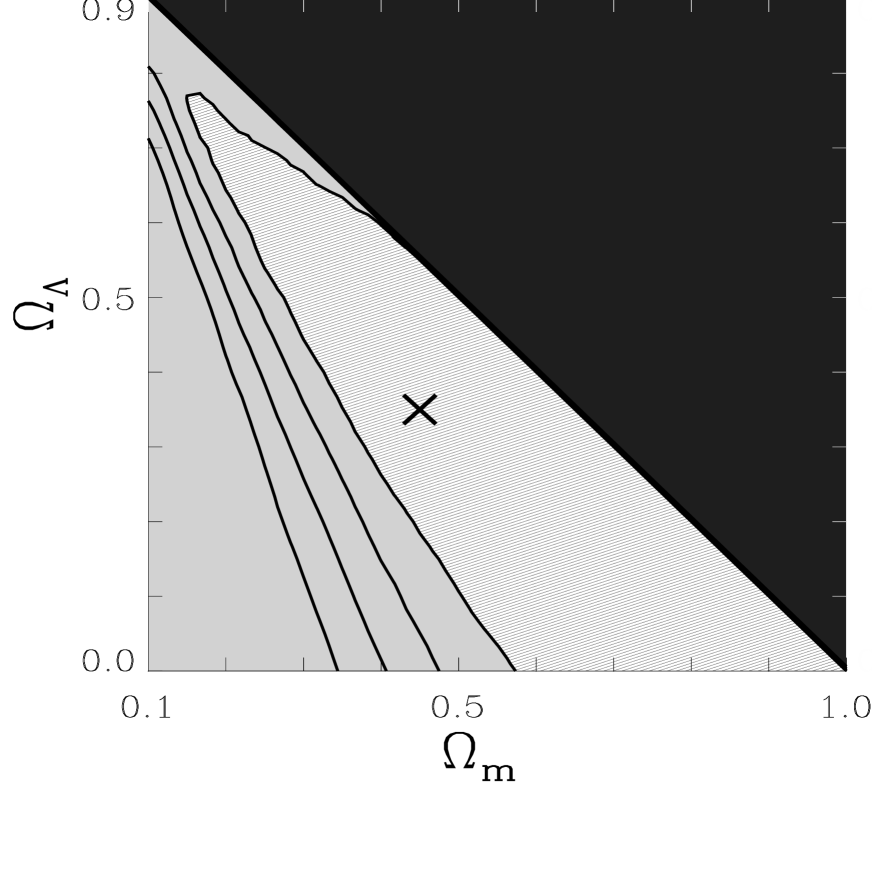
Figure 2: The current CMB data prefer the narrow hashed triangular region (68.3% confidence level) enclosed by approximate $95.4\%,99.7\%$ and $99.9\%$ contours. The ‘X’ marks the best fit: $({\Omega_{m}},{{\Omega_{\Lambda}}})=(0.45,0.35)$. This region is bounded by the limits: ${{\Omega_{\Lambda}}}<0.77$ and ${\Omega_{m}}>0.15$. Assuming ${{\Omega_{\Lambda}}}=0$, yields the lower limit ${\Omega_{m}}>0.57$. Restricting consideration to flat-${\Lambda}$ models, the best-fit is ${{\Omega_{\Lambda}}}=0.1$ with an upper limit ${{\Omega_{\Lambda}}}<0.61$.

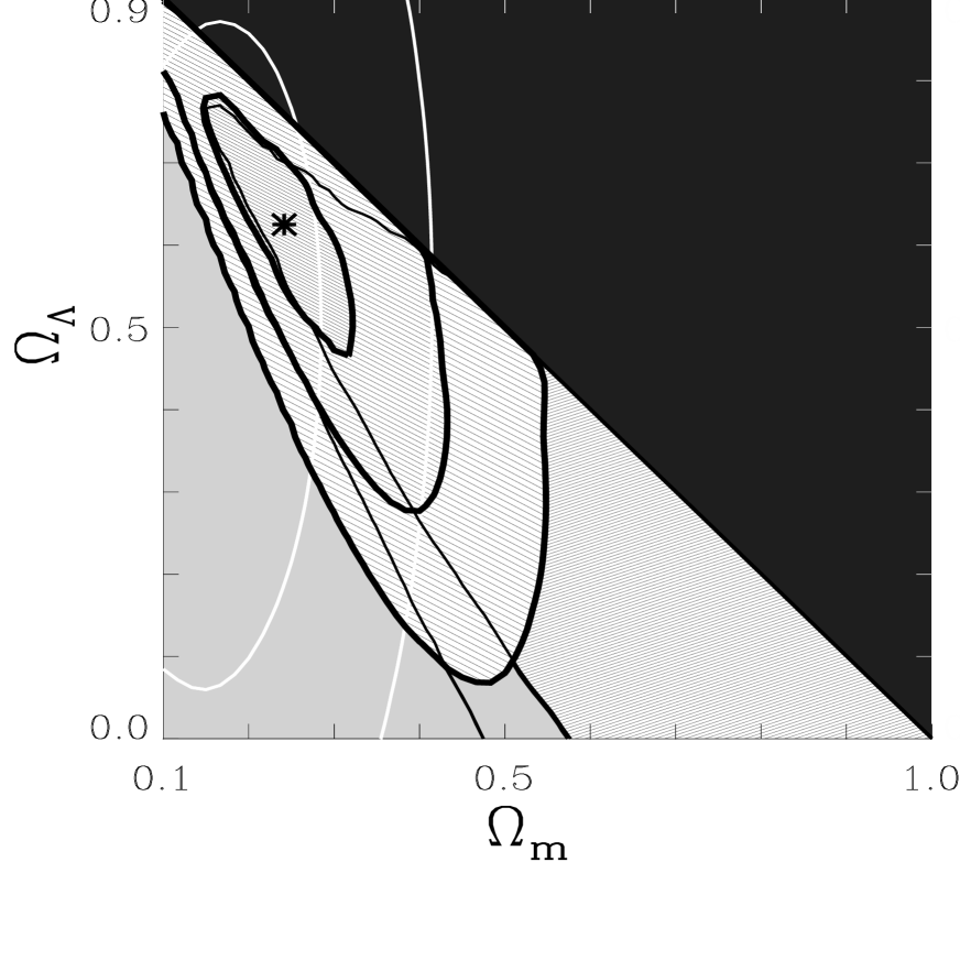
Figure 3: The thick dark lines are the approximate $68.3\%$, $95.4\%$ and $99.7\%$ contours from the joint likelihood of the CMB and non-CMB constraints. The $68.3\%$ and $95.4\%$ confidence levels from non-CMB observations are in white (same as in Figure 1). The $68.3\%$ and $95.4\%$ confidence levels from CMB observations are the thin black lines (same as in Figure 2 but partially obscured here). The best fit is : ${\Omega_{m}}=0.24\pm 0.10$ and ${{\Omega_{\Lambda}}}=0.62\pm 0.16$. ${{\Omega_{\Lambda}}}=0$ models are excluded at more than the $99.7\%$ confidence level.

References

- Baker (1997) Baker, J. 1997, in Proc. of Conf Particle Physics and the Early Universe ed. R. Batley, M. Jones & D. Green (Cambridge:Mullard Radio Astronomy Observatory)
- (2) Bartlett, J. et al. 1998, Fundamental Parameters in Cosmology, Moriond Proceedings, eds. J. Tran Thanh Van & Y.Giraud-heraud (Paris:Editions Frontieres) 1998, astro-ph/9804158
- (3) Bond, J. R. & Jaffe, A.H. 1997, Microwave Background Anisotropies, Proc. of the XVIth Moriond Astrophysics Meeting, edt. F.R.Bouchet et al. , Editions Frontieres, p. 197
- (4) Bond, J.R. et al. 1997, MNRAS, 291, 33
- car (97) Carlberg, R.G. et al. 1997, Ap.J. , 478, 462
- car (98) Carlberg, R.G. et al. 1998, astro-ph/9804312
- car (92) Carroll, S.M. et al. 1992, ARAA, 30, 499
- chi (97) Chiba, M. & Yoshii, Y. 1997, Ap.J. , 490, L73
- (9) Daly, R. et al. 1998, Fundamental Parameters in Cosmology, Moriond Proceedings, eds. J. Tran Thanh Van & Y.Giraud-heraud (Paris:Editions Frontieres), astro-ph/9803265
- deB (97) deBernardis, P et al. 1997, Ap.J. , 480, 1
- (11) Dekel, A. et al. 1997, in “Critical Dialogs in Cosmology”, edt. N. Turok, in press, (Princeton: PUP), astro-ph/9705033
- Ein (17) Einstein, A. 1917, Sitz. Preuss. Akad. Wiss.; translation in H.A.Lorentz et al. Principle of Relativity (Dover:New York) 1952, pp 175-188
- Fal (98) Falco, E.E., Kochanek, C., & Muñoz 1998, Ap.J. , 494, 47
- fel (86) Felten, J.E. & Isaacman, R. 1986, Rev. Mod. Phys. 58, 689
- Femenia et al. (1998) Femenía, B. et al. 1998, Ap.J. , 498, 117
- fer (98) Ferreira, P.G. et al. 1998, 503, L1, astro-ph/9803256
- for (97) Fort B. et al. 1997, A&A, 321, 353
- gar (98) Garnavich, P.M. et al. 1998, Ap.J. , 493, L53
- han (98) Hancock, S. et al. 1998, MNRAS, 294, L1
- Ho (96) Hogan, C.J. astro-ph/9609138
- (21) Jungmann, G. et al. 1996, Phys. Rev. D., 54, 1332
- (22) Kochaneck, C. 1996, Ap.J. , 466, 638
- Leitch (1998) Leitch, E.M. 1998, Ph.D. thesis, California Institute of Technology
- (24) Lesgourgues, J. et al. 1998, MNRAS, in press, astro-ph/9711139
- (25) Lineweaver, C.H. et al. 1997, A&A, 322, 365
- (26) Lineweaver, C.H. & Barbosa, D. 1998a, A&A, 329, 799
- (27) Lineweaver, C.H. & Barbosa, D. 1998b, Ap.J. , 496, 624
- (28) Lineweaver, C.H. 1998, astro-ph/9803100, Proc. of ESO/Australia Looking Deep in the Southern Sky, edt R. Moganti, W. Couch, (Springer:Berlin), 1998, in press
- Netterfield et al. (1997) Netterfield, C. B. et al. 1997, Ap.J. , 474, 47
- (30) Ostriker, J.P. & Steinhardt, P.J. 1995, Nature, 377, 600
- (31) Peacock, J.A. 1998, Phil. Trans. R. Soc London A, submitted, astro-ph/9805208
- (32) Peebles, P.J.E. 1998, astro-ph/9805212
- (33) Perlmutter, S. et al. 1997, Ap.J. , 483, 565
- (34) Perlmutter, S. et al. 1998, Nature, 391, 51
- (35) Perlmutter, S. (private communication) & B.A.A.S. v.29 n.5 p 1351, http:/www-supernova.lbl.gov
- Piccirillo et al. (1993) Piccirillo, L. & Calisse P. 1993, Ap.J. , 411, 529
- (37) Ratra, B. et al. 1997, Ap.J. , 481, 22
- (38) Riess, A.G. et al. 1998, AJ, in press, astro-ph/9805201
- Roos (1998) Roos, M. & Harun -or-Rachid, S.M. 1998, A&A, 329, L17,
- (40) Sarkar, S., 1996, Rep. Prog. Phys., 59, 1493
- (41) Schmidt, B.P. et al. 1998, Ap.J. , in press, astro-ph/9805200
- (42) Scott, D., Silk, J. & White, M. 1995, Science, 268, 829
- (43) Seljak, U. & Zaldarriaga, M. 1996 Ap.J. , 469, 437
- Tanaka (1997) Tanaka, S.T., private communication
- Tegmark et al. (1997) Tegmark, M. & Hamiliton, A. 1997, astro-ph/9702019
- (46) Turner, M.S. 1991, Proc. of the IUPAP Conf. on Primordial Nucleosynthesis and the Early Evolution of the Universe, ed. K. Sato (Kluwer:Dordrecth)
- (47) Webster, M. et al. 1998, Ap.J. , submitted, astro-ph/9802109
- (48) White, M. 1998, Ap.J. , in press, astro-ph/9802295
- (49) Zaldarriaga, M., Spergel, D. & Seljak, U. 1997, Ap.J. , 488, 1