Stability of Power-Law Disks II – The Global Spiral Modes

Abstract

This paper reports on the in-plane normal modes in the self-consistent and the cut-out power-law disks. Although the cut-out disks are remarkably stable to bisymmetric perturbations, they are very susceptible to one-armed modes. For this harmonic, there is no inner Lindblad resonance, thus removing a powerful stabilising influence. A physical mechanism for the generation of the one-armed instabilities is put forward. Incoming trailing waves are reflected as leading waves at the inner cut-out, thus completing the feedback for the swing-amplifier. Growing three-armed and four-armed modes occur only at very low temperatures. However, neutral $m=3$ and $m=4$ modes are possible at higher temperatures for some disks. The rotation curve index $\beta$ has a marked effect on stability. For all azimuthal wavenumbers, any unstable modes persist to higher temperatures and grow more vigorously if the rotation curve is rising ($\beta<0$) than if the rotation curve is falling ($\beta>0$). If the central regions or outer parts of the disk are carved out more abruptly, any instabilities become more virulent.

The self-consistent power-law disks possess a number of unusual stability properties. There is no natural time-scale in the self-consistent disk. If a mode is admitted at some pattern speed and growth rate, then it must be present at all pattern speeds and growth rates. Our analysis – although falling short of a complete proof – suggests that such a two-dimensional continuum of non-axisymmetric modes does not occur and that the self-consistent power-law disks admit no global non-axisymmetric normal modes whatsoever. Without reflecting boundaries or cut-outs, there is no resonant cavity and no possibility of unstable growing modes. The self-consistent power-law disks certainly admit equiangular spirals as neutral modes, together with a one-dimensional continuum of growing axisymmetric modes.

• Key words: celestial mechanics, stellar dynamics – galaxies: kinematics and dynamics – galaxies: structure – galaxies: spiral

1 Introduction

The preceding paper in Monthly Notices has presented the formidable machinery to permit direct solution for the in-plane normal modes of the family of razor-thin power-law disks. The results in this paper are based on a fast computer program that sets this machinery working.

The entire spectrum of normal modes of a family of rigidly rotating stellar dynamical disks was deduced by Kalnajs [Kalnajs 1972] in a bravura piece of mathematical analysis using “only pencil, paper and Legendre polynomials” [Toomre 1977]. Differentially rotating disks are much harder and the results in the literature are sparse. Kalnajs [Kalnajs 1977] devised a general procedure for deducing the normal modes of an axisymmetric stellar disk using matrix mechanics in action-angle coordinates and he subsequently applied his method to the isochrone disk [Kalnajs 1978]. Over twenty years have passed since Zang’s [Zang 1976] thesis on the scale-free disk with a completely flat rotation curve, yet it remains the most complete and instructive normal mode analysis available. In fact – perhaps daunted by the complexities of mode analyses – many researchers have looked for convenient short-cuts, such as gas approximations [Bardeen 1978, Aoki et al. 1979, Bertin & Lin 1996] or the use of cold disks with softened gravity [Erickson 1974, Toomre 1981] or the combination of N-body work with approximate analytic treatments [Sellwood 1989]. Our aim is to extend Zang’s normal mode work to all the scale-free disks with rising and falling rotation curves, the power-law disks. We are not alone in fixing attention on these disks as suitably simple models for which global stability analyses can be carried out. The gaseous power-law disks have attracted the attentions of a number of investigators [Schmitz & Ebert 1987, Lemos et al. 1991, Lynden-Bell & Lemos 1993, Syer & Tremaine 1996]. The present paper gives a complete analysis of the global stability of the cut-out and the self-consistent power-law disks of stars. In the cut-out disks, stars close to the centre (and sometimes also at large radii) are prevented from participating in the disturbance. In the self-consistent disks, all the stars are mobile.

Our study of the global stability of the cut-out power-law disks aims to determine how much random motion is required to stabilise a disk to modes of each angular harmonic. A recurring theme of numerical simulations throughout the seventies and eighties has been the ferocity of the bar instability, even in disks that are safely stable to axisymmetric perturbations [Hohl 1971, Athanassoula & Sellwood 1986, Sellwood & Wilkinson 1993]. Zang [Zang 1976], somewhat surprisingly, found that this is not the case for the scale-free disk with a flat rotation curve. It is bar-stable unless so cold that it is already susceptible to axisymmetric modes. For each power-law disk, it is interesting to locate the fastest growing modes and establish the physical origin of the instabilities. Are galaxies with rising rotation curves more or less stable than galaxies with falling curves? What kinds of density laws can be carved out to render a disk stable (or unstable)? As exact global stability analyses will remain scarce because of their cumbersome nature, it is important to assess how rules-of-thumb – such as Toomre’s [Toomre 1964] local criterion, or Ostriker and Peebles’ [Ostriker & Peebles 1973] global criterion – fare against exact results.

The behaviour of the self-consistent disks must be very different from that of the cut-out disk. As originally pointed out by Kalnajs in 1974 (reported in Zang (1976)), all dependence on growth rate and pattern speed can be factored out of the integral equation for the normal modes. The same detail was noted independently by [Lynden-Bell & Lemos 1993] using an argument based on dimensional analysis. Physical intuition suggests that as a disk is cooled below the critical temperature, growing modes become possible. But, the symmetry of the scale-free disk forbids a preference for one growth rate over another. At the critical temperature, the disk must admit modes with all frequencies or none. Thus, there seem to be two options: either there is a continuum of modes with all possible pattern speeds and growth rates, or there are no normal modes whatsoever. Do the scale-free, self-consistent power-law disks have normal modes? There are contradictory speculations on the answer to this question [Zang 1976, Lynden-Bell & Lemos 1993].

The paper first concentrates on the cut-out disks and examines their global stability according to azimuthal wavenumber. Bisymmetric instabilities ($m=2$) are studied in Section 3. The one-armed modes ($m=1$) are examined in Section 4, while the other azimuthal harmonics ($m=3,4$) in Section 5. Finally, Section 6 considers the self-consistent disk in the light of the insights gained in the study of cut-out disks. Before all this, however, we begin with a short introductory Section 2, which introduces some common notation and themes for the rest of the paper.

2 Theoretical Preamble

Before discussing stability to any non-axisymmetric modes, it is helpful to start with a brief discussion of axisymmetric stability. This provides part of the intellectual framework needed to understand the non-axisymmetric results. For short wavelength, axisymmetric modes,  [Toomre 1964] showed that local stability requires that the velocity dispersion exceed a critical value $\tilde{\sigma}_{u,\min}$. First, let us make the convenient abbreviation

$$L(\beta)=\frac{\Gamma\left[{{1\over 2}}\left(1-\beta\right)\right]\Gamma\left[{{1\over 2}}\left(2+\beta\right)\right]}{\Gamma\left[{{1\over 2}}\left(1+\beta\right)\right]\Gamma\left[{{1\over 2}}\left(2-\beta\right)\right]},$$ (1)

For the power-law disks, the critical velocity dispersion for stability to axisymmetric modes is

$$\tilde{\sigma}_{u}>\tilde{\sigma}_{u,\min}=\frac{3.3582830}{2\pi L(\beta)\sqrt{2-\beta}}\frac{\Sigma_{\text{active}}}{\Sigma_{\text{eq}}},$$ (2)

where $\Sigma_{\text{active}}$ is the active surface density or the density spared by the cut-out function and $\Sigma_{\text{eq}}$ is the surface density implied by Poisson’s equation. For the cut-out disks, $\tilde{\sigma}_{u,\min}$ is a function of radius, although for the self-consistent disk it is not. We shall often relate the velocity dispersion $\tilde{\sigma}_{u}$ in both self-consistent and cut-out disks to the minimum velocity dispersion necessary to ensure local axisymmetric stability in the self-consistent disk. This ratio is referred to as $Q_{\text{s}}$

$$Q_{\text{s}}=\tilde{\sigma}_{u}\frac{2\pi\sqrt{2-\beta}}{3.3582830}L(\beta).$$ (3)

Local theory tells us that $Q_{\text{s}}\geq 1$ is sufficient to stabilise against short wavelength axisymmetric modes. This result also holds good for stability against global axisymmetric modes, as has been found before by others [Zang 1976, Lemos et al. 1991] and is briefly demonstrated anew in Appendix A.

$\beta$	$L(\beta)$	$mX$	$\tilde{\sigma}_{u,\min}$
$-0.75$	$0.233406$	$0.641867$	$1.380888$
$-0.5$	$0.456947$	$1.142366$	$0.739779$
$-0.25$	$0.700219$	$1.575492$	$0.508877$
$0.0$	$1.000000$	$2.000000$	$0.377940$
$0.25$	$1.428125$	$2.49929$	$0.282912$
$0.5$	$2.188440$	$3.282660$	$0.199415$
$0.75$	$4.284375$	$5.355469$	$0.111582$

Table 2: This table shows the variation of some useful stability indicators with the rotation curve index $\beta$ of the self-consistent power-law disks. Here, $\tilde{\sigma}_{u,\min}$ is the minimum velocity dispersion (measured relative to the local circular speed) needed to suppress axisymmetric Jeans instabilities entirely. $X$ is the ratio of the circumferential wavelength of an $m$-armed disturbance to the longest Jeans unstable wavelength $\lambda_{\rm crit}$ in a cold disk.

Toomre (1964) showed that rotation alone stabilises axisymmetric modes with wavelengths in excess of $\lambda_{\rm crit}$

$$\lambda_{\rm crit}={4\pi^{2}G\Sigma\over\kappa^{2}}={2\pi R\over(2-\beta)L(\beta)}{\Sigma_{\text{active}}\over\Sigma_{\text{eq}}}.$$ (4)

Equivalently, lengthscales larger than $\lambda_{\rm crit}$ are stable to Jeans instabilities even in a cold disk. It is often helpful to discuss non-axisymmetric instabilities in terms of a dimensionless ratio $X$ (e.g., Toomre 1981). This is the ratio of the circumferential wavelength of an $m$-armed disturbance $\lambda$ to $\lambda_{\rm crit}$, i.e.,

$$X=\frac{\lambda}{\lambda_{\rm crit}}={2\pi R\over m\lambda_{\rm crit}}=\frac{(2-\beta)L(\beta)}{m}{\Sigma_{\text{eq}}\over\Sigma_{\text{active}}}.$$ (5)

Table 1 shows how these helpful stability parameters vary for the self-consistent power-law disks ($\Sigma_{\text{eq}}=\Sigma_{\text{active}}$). The table makes the point that the properties of the disks change quickly as one moves away from the reference Toomre-Zang disk ($\beta=0$). For example, $\lambda_{\rm crit}$ increases by a factor of $1.75$ on moving from $\beta=0$ to $\beta=-0.5$ and decreases by a factor of $1.64$ on passing from $\beta=0$ to $\beta=0.5$. The densities of any clumps formed simply through axisymmetric Jeans instabilities are almost a factor of three larger on moving from $\beta=0.5$ to $\beta=-0.5$. Relative to the local circular speed, $\tilde{\sigma}_{u,\min}$ roughly doubles or halves on making the same journeys. This table already suggests that the disks with $\beta<0$ will be harder to stabilise against Jeans instabilities and their kin than the disks with $\beta>0$. The swing-amplifier is at its fiercest when $1\mathrel{\hbox to0.0pt{\lower 3.0pt\hbox{$\sim$}\hss}\raise 2.0pt\hbox{$<$}}X\mathrel{\hbox to0.0pt{\lower 3.0pt\hbox{$\sim$}\hss}\raise 2.0pt\hbox{$<$}}2$ and becomes weak once $X>3$ (see Toomre 1981). So, Table 1 cautions us that the one-armed ($m=1$) modes especially in the disks with rising rotation curves ($\beta<0$) will be particularly troublesome to stabilise.

3 Bisymmetric Modes

This section provides the results of the stability analysis to global bisymmetric perturbations. From an observational standpoint, these are the most important, as some $30\%$ of disk galaxies are strongly barred with perhaps a further $30\%$ showing evidence of weaker barring [Sellwood & Wilkinson 1993]. There are even galaxies known which are unbarred in the optical but are barred in the infrared. Approximate bisymmetry is a characteristic of most disk galaxies.

3.1 The Behaviour of the Eigenvalues

3.1.1 The Effect of Growth Rate and Pattern Speed

Let us recall that the mathematical eigenvalue $\lambda$ is the ratio of the response to the imposed density transforms (see Section 4.3 of the preceding paper). Mathematically, it is defined by $A_{\text{res}}(\alpha)=\lambda A_{\text{imp}}(\alpha)$. If the modulus of the complex mathematical eigenvalue $|\lambda|$ is greater than unity, the response is more vigorous than the imposed perturbation. If $|\lambda|<1$, the response is less than the original disturbance. When the mathematical eigenvalue is unity, the response is identical in magnitude and phase to the imposed disturbance. This is a self-consistent mode. To discover global modes, it is important to understand the position of the eigenvalue in the complex plane and to learn what choices of growth rate, pattern speed and temperature can bring it to the point $(1,0)$. Cool disks are (usually) less stable than warm ones. By increasing the temperature sufficiently, the modulus of the mathematical eigenvalue shrinks so that no choice of growth rate $s$ and pattern speed $\Omega_{\text{p}}$ enables it to attain the value $(1,0)$. On physical grounds, slowly-growing disturbances are expected to be more easily excited than faster ones. Thus, the modulus of the mathematical eigenvalue is greater for smaller growth rates. The pattern speed has a twofold effect, as it controls the phase of the response and determines the position of the co-rotation radius $R_{\text{CR}}$ and the inner and outer Lindblad resonances, $R_{\text{ILR}}$ and $R_{\text{OLR}}$. For the power-law disks, these crucial radii occur at:

$$\frac{R_{\text{ILR}}}{R_{0}} =\left(\frac{m-\sqrt{2-\beta}}{m\tilde{\Omega}_{\text{p}}}\right)^{\frac{2}{2+\beta}}, \quad\frac{R_{\text{OLR}}}{R_{0}} =\left(\frac{m+\sqrt{2-\beta}}{m\tilde{\Omega}_{\text{p}}}\right)^{\frac{2}{2+\beta}}, \quad\frac{R_{\text{CR}}}{R_{0}} =\left(\frac{1}{\tilde{\Omega}_{\text{p}}}\right)^{\frac{2}{2+\beta}}.$$ (6)

These formulae are given for general azimuthal wavenumber $m$. Henceforth, the emphasis in this section is on $m=2$. Any modes are generally confined to the region between the two Lindblad resonances. For $\tilde{\Omega}_{\text{p}}\gtrsim 1+\textstyle{1\over 2}\displaystyle\sqrt{2-\beta}$, the outer Lindblad resonance lies inside the inner cut-out at $R=R_{0}$. The disturbance is restricted to a part of the disk where there is not much matter free to respond. The response, and hence the mathematical eigenvalue, is expected to be small for large pattern speeds. For $\tilde{\Omega}_{\text{p}}\lesssim 1-\textstyle{1\over 2}\displaystyle\sqrt{2-\beta}$, the inner Lindblad resonance lies beyond the inner cut-out. Now, the presence of the inner cut-out has a minimal effect on the response, since the density experienced is similar to that in the self-consistent disk. Each imposed logarithmic spiral then excites only a pure logarithmic spiral in response and so the eigenvalue is expected to be real. In a doubly cut-out disk, with sufficiently low pattern speed, the inner Lindblad resonance can fall beyond the outer cut-off at $R=R_{\text{c}}$. In this case, the mathematical eigenvalue is again expected to be very small.

Fig. 2 shows the effect of growth rate and pattern speed on the mathematical eigenvalue for $N=2$ disks with $\beta=\pm 0.25$. The temperature of each disk is chosen so that it is locally stable to axisymmetric perturbations, i.e., $Q_{\text{s}}=1$.

Figure 2: The dependence of the largest mathematical eigenvalue on growth rate and pattern speed for bisymmetric disturbances in a inner cut-out disk with $N=2$, $Q_{\text{s}}=1$ and $\beta=\pm 0.25$. [The solid lines show curves of constant $s$ at intervals of 0.1 from $s=0^{+}$ to $s=0.5$. The dotted lines show curves of constant $\Omega_{\text{p}}$ at intervals of 0.1 from $\Omega_{\text{p}}=0.5$ to $\Omega_{\text{p}}=2.0$. For $\beta=0.25$, $\tilde{\sigma}_{u}=0.283$ and $\gamma=11.0$; for $\beta=-0.25$, $\tilde{\sigma}_{u}=0.509$ and $\gamma=3.36$].

The curves have the general behaviour expected from our theoretical discussion. As the pattern speed is increased beyond $\sim 1$, the modulus of the mathematical eigenvalue declines. For large $\Omega_{\text{p}}$, the eigenvalue turns towards the origin and the growth rate becomes smaller. The disk responds to the perturbation rather weakly, since most of the mass has been removed from the central region. Now, the mathematical eigenvalue depends on growth rate $s$ and pattern speed $\Omega_{\text{p}}$ through the single complex frequency $\omega=m\Omega_{\text{p}}+is$. Since the kernel is analytic, the mathematical eigenvalue $\lambda$ is an analytic function of $\omega$. As realised by Zang [Zang 1976], this means that $\lambda(\omega)$ gives a conformal mapping of the upper half of the complex $\omega$-plane (since the growth rate is positive) to the complex $\lambda$-plane. Conformal mappings preserve the angles of infinitesimal polygons. So, curves of constant $s$ and constant $\Omega_{\text{p}}$ are orthogonal. Fig. 2 shows a problem which can occur. For $\beta=0.25$, there is a discontinuity near ($\Omega_{\text{p}}=0.5$, $s=0.4$), even though $\lambda$ is expected to change smoothly. The discontinuity arises because here the second largest eigenvalue overtakes the previously largest one, so that the same eigenvalue is not being followed.

What are the values of the growth rate, pattern speed and temperature for which the eigenvalue is unity? Fig. 2 already suggests that, for $Q_{\text{s}}=1$ disks with $\beta$ in the range $-0.25$ to $0.25$, no choice of growth rate and pattern speed results in an eigenvalue equal to unity. For each $\beta$, the curves of constant growth rate cross the real axis well to the left of unity. From our theoretical discussion, the mathematical eigenvalue is likely to continue towards the origin as the pattern speed increases still further. Assuming that, at any pattern speed, the marginal eigenvalue curve has the largest modulus and that the curves of constant $s$ do not cross, it seems improbable that any solutions can exist at pattern speeds lower than those shown. Fig. 2 plots the behaviour of the dominant eigenvalue, i.e., that which has the largest modulus at a particular pattern speed and growth rate. For the range of pattern speeds investigated so far, the modulus of the dominant eigenvalue has not reached unity, and so none of the lower eigenvalues can yield a mode. Let us also observe from Fig. 2 that as $\beta$ is reduced from $0.25$ to $-0.25$, the set of curves tilts upwards, crossing the real axis at higher values, and thus coming closer to possessing a unit eigenvalue. The disks with rising rotation curves (negative $\beta$) are less securely stable than their relatives with falling rotation curves (positive $\beta$). Fig. 4 shows marginal eigenvalue curves for several different values of $\beta$ in the range $-0.5$ to $+0.35$. The curves are drawn for $Q_{\text{s}}=1$, so all the disks shown are already stable to axisymmetric perturbations. The disks with rising rotation curves have higher velocity dispersions than those with falling rotation curves, but even so they are more prone to bisymmetric disturbances. As $\beta$ is decreased, the magnitude of the marginal eigenvalue at a given pattern speed increases. Eigenvalues in disks with rising rotation curves cross the real axis at higher values than for their cousins with falling rotation curves.

Figure 4: Marginal eigenvalue curves for bisymmetric disturbances in inner cut-out disks with $N=2$ and values of the rotation curve index from $\beta=-0.5$ to $\beta=0.35$ in steps of 0.05. The velocity dispersion for each $\beta$ is that corresponding to local axisymmetric stability ($Q_{\text{s}}=1$). [The plot shows the largest mathematical eigenvalues for vanishing growth rate, $s=10^{-7}$, and 20 values of the pattern speed: $\Omega_{\text{p}}=0.0001$, 0.0005, 0.001, 0.005, 0.01, 0.02, 0.05, 0.1, 0.2, 0.3, $\dots$ 1.2, 1.3.]

For values of $\beta<-0.470$, $Q_{\text{s}}=1$ is insufficient to stabilise the disk to $m=2$ perturbations. Disks whose rotation curves rise faster than this succumb to bar-like modes, even if stable to axisymmetric modes.

3.1.2 The Effect of the Temperature and the Inner Cut-Out

Raising the velocity dispersion $\tilde{\sigma}_{u}$ moves the marginal stability curves closer to the origin, while lowering it moves them further out. At some value $\tilde{\sigma}_{u,\min}$, the marginal stability curve will pass through (1,0); this is the temperature at which the disk is just stable to bisymmetric perturbations. Fig. 6 shows how the temperature affects the marginal stability curve. The eigenvalue depends separately on the pattern speed and temperature, so the mapping from the ($\Omega_{\text{p}}$-$Q_{\text{s}}$) plane to the complex $\lambda$ plane is not conformal. This is evident from Fig. 6, where lines of constant $\Omega_{\text{p}}$ and constant $Q_{\text{s}}$ do not intersect at right-angles. Again, this demonstrates that power-law disks with falling rotation curves are securely stable to bisymmetric perturbations. Even when the velocity dispersion is only 60% of that needed for axisymmetric stability, the $\beta=0.25$ disk admits no $m=2$ modes.

Figure 6: The dependence of the largest mathematical eigenvalue on temperature and pattern speed for inner cut-out disks with $\beta=\pm 0.25$. Curves are plotted for bisymmetric perturbations with vanishing growth rate in a disk with cut-out index $N=2$. The temperature used for each curve is expressed in terms of $Q_{\text{s}}$. [For $\beta=0.25$, $\tilde{\sigma}_{u}=0.283Q_{\text{s}}$; for $\beta=-0.25$, $\tilde{\sigma}_{u}=0.509Q_{\text{s}}$].

The inner cut-out strongly influences the stability of the disk (c.f., Zang 1976; Toomre 1977). To illustrate this, Fig. 8 shows the marginal stability curves in disks with different $\beta$ and different values of the inner cut-out index $N$.

Figure 8: The dependence of the largest mathematical eigenvalue on pattern speed, for different inner cut-out indices $N$. Curves are plotted for bisymmetric perturbations with vanishing growth rate in an inner cut-out disk with $\beta=\pm 0.25$. The curves are labelled with the value of the inner cut-out index $N$. [In each case $Q_{\text{s}}=1$. The diamonds show the results for $\Omega_{\text{p}}=0.1$, 0.2, 0.3 … 2.0.]

Increasing the cut-out index $N$ makes the disk much more susceptible to instabilities. Curves with higher $N$ cross the real axis at successively higher values of $\lambda$. Disks with $N=1$ are highly stable to $m=2$ perturbations. To understand why the inner cut-out has such a profound effect on the stability of the disks, let us consider the position of the Lindblad resonances. For low values of the pattern speed, the inner Lindblad radius lies outside the inner cut-out radius $R_{0}$. Incoming waves are absorbed by the inner Lindblad resonance, which thus damps disturbances in the disk and reduces the possibility of a mode. However, once $\Omega_{\text{p}}$ exceeds $\sim 0.25$, the inner Lindblad resonance moves inside the inner cut-out radius. If the cut-out is gentle ($N=1$), the incoming waves pass through it, reach the inner Lindblad resonance and are absorbed. If however the cut-out is sufficiently sharp (as for larger cut-out indices), it presents a barrier which reflects the incoming trailing waves. Instead of reaching the inner Lindblad resonance and being absorbed, they are reflected back as outgoing leading waves. The exceptional stability of $N=1$ disks is mostly due to the fact that the surface density is disturbed much less abruptly than for higher cut-out indices, presenting less of a reflective barrier to incoming waves. Additionally, there is a much greater surface density within the inner cut-out when $N=1$; the active surface density diverges at the origin when the rotation curve is falling, and even when the rotation curve is rising, the surface density remains large to much smaller radii. By contrast, for $N>1$, the active surface density rapidly falls to zero within $R_{0}$. Waves are thus suppressed by simply having no medium through which to propagate.

3.2 The Marginal Modes

The marginal modes are those with vanishingly small growth rate. How cold does the disk have to be for this transition from stability to instability to occur? This question can be answered by finding the temperature for which the marginal eigenvalue curve passes through $(1,0)$. Fig. 10 shows the minimum temperature needed for bisymmetric stability as a function of $\beta$. The solid lines show the results for the inner cut-out disks with $N=2$, 3, and 4. The broken lines show results for the corresponding doubly cut-out disks with $M=2$, 4, 6 and $\tilde{R}_{\text{c}}=10$.

Figure 10: Minimum temperature for bisymmetric stability plotted against rotation curve index $\beta$ for disks with various cut-out functions. The left-hand plot shows the minimum velocity dispersion $\tilde{\sigma}_{u}$; the right-hand one the same data presented in terms of the stability parameter $Q_{\text{s}}$. The solid lines indicate the results for inner cut-out disks with $N=1$, 2, 3, 4. The broken lines indicate the corresponding doubly cut-out disks with $M=2$, 4, 6 and $\tilde{R}_{\text{c}}=10$.

Curves with different $N$ lie well apart. The more sharply the core is cut out, the more unstable the disk becomes. For each $N$, the curves with different $M$ lie very close together. Even with this low truncation radius, the outer cut-out function makes little difference to the temperature necessary for stability. With a larger $\tilde{R}_{\text{c}}$, the doubly cut-out curves are scarcely distinguishable from those with only an inner cut-out. The right-hand plot in Fig. 10 can be used to compare the relative stability of the various cut-out disks to $m=0$ and $m=2$ perturbations. The $N=2$ disk is less prone to bisymmetric than to axisymmetric instabilities over almost all $\beta$. For $N=3$, the relative tendency to $m=2$ and $m=0$ disturbances depends on $\beta$. Roughly speaking, $N=3$ disks with rising rotation curves are more susceptible to $m=2$ disturbances whereas disks with falling rotation curves are more susceptible to $m=0$. Conversely, disks with $N=4$ are much more prone to bisymmetric disturbances over almost all $\beta$. Only when the rotation curve is steeply falling does the $m=0$ mode become harder to stabilise. It is perhaps surprising that it is the lowest outer cut-out index ($M=2$) which shows the largest departure from the inner cut-out curves. In this instance, it seems that tapering the disk gently at large radius has more of an effect than truncating it abruptly. This is presumably because for lower $M$, the effect of the outer cut-out is felt further in towards the centre of the disk. For higher $M$, the outer cut-out is sharp, but occurs entirely outside the outer Lindblad resonance. Disks with a gentle outer cut-out are more stable than those where the cut-out is sharper. The critical pattern speed obtained for these marginal modes is shown in Fig. 12. For all cut-out functions and $\beta$, the pattern speed is confined to a fairly narrow range, roughly 0.3 to 0.6. Over a wide range in $\beta$, the pattern speed varies roughly linearly with $\beta$.

Figure 12: Critical pattern speed $\Omega_{\text{p}}$ plotted against rotation curve index $\beta$ for $m=2$ modes in disks with various cut-out functions. The solid lines are labelled with the inner cut-out index $N$. For each $N$, different outer cut-out indices $M$ are plotted.

Let us look at the shapes of some of these marginally stable modes. The contour plots in Fig. 14 show the form of the modes for $\beta=\pm 0.25$ in inner cut-out disks with $N=2$.

Figure 14: Density contour plot of a marginally stable mode in inner cut-out disks with $N=2$. The solid lines mark 10%, 20%, 40%, 60% and 80% of the maximum density. The dotted lines show the nodes, where the perturbation density vanishes. The Lindblad resonances and the co-rotation radius are indicated by dashed circles. [The left-hand plot is for $\beta=0.25$, for which the marginally stable mode has $Q_{\text{s}}=0.500$, $\gamma=48.4$, $\tilde{\sigma}_{u}=0.142$, $\Omega_{\text{p}}=0.596$ and $\alpha_{\text{u}}\approx 20.4$. The right-hand plot is for $\beta=-0.25$, for which the marginally stable mode has $Q_{\text{s}}=0.631$, $\gamma=9.19$, $\tilde{\sigma}_{u}=0.321$, $\Omega_{\text{p}}=0.533$ and $\alpha_{\text{u}}\approx 8.4$].

For falling rotation curves, the modes are more tightly wound than for rising rotation curves. They extend beyond co-rotation up to the outer Lindblad resonance, whereas in disks with rising rotation curves the modes are concentrated between the inner Lindblad resonance and the co-rotation radius. The modes are also more tightly wound for disks with gentle cut-outs. These effects are caused by the higher temperatures needed for marginal modes when the rotation curve is rising. If a growing mode exists, then the stars do not have enough random motion to move entirely out of a density enhancement before it has grown significantly. As the temperature increases, the stars have more random motion, and the spiral modes can therefore be more loosely wound. As shown in Fig. 12, the pattern speed of modes increases with $\beta$ and is greater for disks with lower cut-out indices. Since the Lindblad resonances move inwards as the pattern speed increases, the pattern is concentrated within a smaller radius for $\beta=0.25$ than for $\beta=-0.25$, and similarly for the lower cut-out indices. Fig. 16 shows the position of the Lindblad and co-rotation resonances for modes in cut-out disks.

Figure 16: Position of resonances for marginal $m=2$ modes in cut-out disks with different rotation curve index $\beta$. The dashed horizontal lines show the position of the inner and outer cut-out radii. The pattern speed corresponding to the marginal mode in each disk (Fig. 12) is used to calculate the the resonance radii. The solid lines mark the Lindblad resonances; the dotted line marks co-rotation. [The three plots show results for $N=2$, 3 and 4; each plot shows data for doubly cut-out disks with $M=2$, 4, 6, $\tilde{R}_{\text{c}}=10$].

It is significant that, for every value of $\beta$, the pattern speed is large enough to push the inner Lindblad resonance just inside the inner cut-out. The disk does not admit slowly-rotating growing modes for which the resonance would emerge beyond the cut-out. The resonance is allowed nearer the cut-out when the cut-out is sharper, and hence a more efficient reflector. Similarly, on examining modes in an unstable disk (Read 1997), the fastest-growing modes have the largest pattern speeds. As the pattern speed decreases, allowing the inner Lindblad resonance to move out closer to the cut-out radius, the growth rate slows.

3.3 The Ostriker-Peebles Criterion

Ostriker and Peebles [Ostriker & Peebles 1973] suggested that disk galaxies are stable to bar-like modes only when the ratio of total rotational energy $T$ to total gravitational energy $|W|$ is less than 0.14. The energies $W$ and $T$ for the self-consistent disk are given in Section 2 of Paper I. We thus deduce the ratios as [Evans 1994]:

$$\frac{T}{|W|} =\frac{\Gamma^{2}\left[1+\frac{\gamma}{2}\right]\Gamma^{2}\left[2+\frac{1}{\beta}+\frac{\gamma}{\beta}\right]}{\beta\Gamma^{2}\left[\frac{1}{2}+\frac{\gamma}{2}\right]\Gamma^{2}\left[\frac{5}{2}+\frac{1}{\beta}+\frac{\gamma}{\beta}\right]}, \quad\beta>0,$$ (7)

$$\frac{T}{|W|} =\frac{\Gamma^{2}\left[1+\frac{\gamma}{2}\right]\Gamma^{2}\left[-\frac{3}{2}-\frac{1}{\beta}-\frac{\gamma}{\beta}\right]}{-\beta\Gamma^{2}\left[\frac{1}{2}+\frac{\gamma}{2}\right]\Gamma^{2}\left[-1-\frac{1}{\beta}-\frac{\gamma}{\beta}\right]}, \quad\beta<0,$$ (8)

$$\frac{T}{|W|} =\frac{1}{1+\gamma}\frac{\Gamma^{2}\left[1+\frac{\gamma}{2}\right]}{\Gamma^{2}\left[\frac{1}{2}+\frac{\gamma}{2}\right]}, \quad\beta=0.$$ (9)

Note that the $\beta=0$ result can be derived from the values for $\beta\neq 0$ using a property of the gamma function  [Gradshteyn & Ryzhik 1978, 8.328.2].

Fig. 18 shows the ratio $T/|W|$ calculated for the self-consistent disk (eqs. (7) and (8)). The anisotropy parameter used at each $\beta$ is that needed for marginal stability to bisymmetric modes in the cut-out disk.

Figure 18: Comparison of the results for the cut-out disks with the Ostriker-Peebles criterion. The plot shows the ratio of total rotational energy to total potential energy necessary for marginal stability to bar modes. The solid lines are labelled with the appropriate inner cut-out index $N$. For each $N$, different outer cut-out indices $M$ are plotted, as shown in the key.

Note that $T/|W|$ can exceed 0.5, since the standard form of the virial theorem does not apply to the power-law disks, which are of infinite extent. For all the disks, the ratio $T/|W|$ is much greater than the value of 0.14 suggested by Ostriker and Peebles. This demonstrates that the Ostriker-Peebles criterion is not useful in predicting the stability of the power-law disks. However, the temperatures used in Fig. 18 are derived for the cut-out disks. As the self-consistent and cut-out disks have different stability properties, perhaps the value of $T/|W|$ should be calculated for the cut-out disks. In this case, the density $\Sigma$ and streaming velocity $\langle v\rangle$ must be computed numerically using the cut-out distribution function. Details of this calculation are given in Read (1997) – there is only a small change in the ratio $T/|W|$ and the main conclusion of this Section is unaffected. For the power-law disks, the Ostriker-Peebles criterion is untrustworthy as it greatly overestimates the amount of energy in the form of random motion necessary to achieve stability against bar modes.

4 One-armed modes

The observational motivation for studying one-armed modes is that mild lop-sidedness is seen in many spiral galaxies, with substantial asymmetries present in some late-type galaxies [Baldwin et al. 1980]. This is evident in both the optical and HI data [Richter & Sancisi 1994, Rix & Zaritsky 1995]. One-armed disturbances differ from many-armed disturbances in one crucial respect. It is intuitively clear that one-armed patterns can move the barycentre from the origin towards the overdense spiral arm. For an isolated system, acceleration of the barycentre is not physical. The possibility occurs here because the analysis holds the equilibrium disk fixed while imposing a perturbation on it. If one-armed waves grow in a galaxy, the equilibrium disk is displaced to balance the perturbation so that the barycentre remained fixed. Our analysis thus reproduces a famous mistake by Maxwell in his Adams Prize essay [Maxwell 1859]. A complete study of the $m=1$ modes requires that our analysis be modified to permit the barycentre to move. Instead, we investigate the stability of the disk to “naïve” one-armed disturbances and check a posteriori that the barycentre moves only slightly. In this, we are in the good company of Toomre and Zang, who did exactly this in their analysis of the disk with a flat rotation curve.

4.1 The Behaviour of the Eigenvalues

Let us first investigate how the largest mathematical eigenvalue depends on pattern speed and growth rate for the temperature at which the self-consistent disk is locally just stable to axisymmetric disturbances. Fig. 20 shows the eigenvalue curves for a disk with $\beta=0.25$ and $N=2$.

Figure 20: The dependence of the largest mathematical eigenvalue on growth rate and pattern speed for one-armed disturbances in inner cut-out disks with $N=2$ and $Q_{\text{s}}=1$. The horizontal axis is $\text{Re}[\lambda]$ and the vertical axis is $\text{Im}[\lambda]$. [In the plot, $\beta=0.25$ ($\tilde{\sigma}_{u}=0.283$ and $\gamma=11.0$). The solid lines show curves of constant $s$ at 11 values of $s$: $s={10}^{-7}$, 0.0001, 0.0005, 0.001, 0.005, 0.01, 0.05, 0.1, 0.2, 0.3, 0.4. The dotted lines show curves of constant $\Omega_{\text{p}}$ at 20 values of $\Omega_{\text{p}}$: $\Omega_{\text{p}}=0.0001$, 0.0005, 0.001, 0.005, 0.01, 0.02, 0.05, 0.1, 0.2, 0.3 $\dots$ 1.2, 1.3].

For growing perturbations ($s\gtrsim 0.05$), these curves are qualitatively similar to those obtained for bisymmetric perturbations (Fig. 2). Curves of a given $s$ cross the real axis at higher values for these $m=1$ plots than for the earlier $m=2$ plots, indicating that the disk is more prone to one-armed than two-armed disturbances. For instance, we saw in Fig. 2 that $Q_{\text{s}}=1$ was already sufficient to stabilise the $\beta=0.25$ disk to $m=2$ disturbances. But, Fig. 20 indicates that this disk remains susceptible to $m=1$ disturbances. One such mode is indicated by the dashed line. The most striking difference between the present situation and that for $m=2$ occurs as the growth rate is reduced to zero. It appears that in the limit of vanishing growth rate, the marginal eigenvalue curves never cross the real axis. Eigenvalues for small but non-zero growth rate (e.g. $s=10^{-4},10^{-3}$) follow the marginal curve for high pattern speeds. As the pattern speed is reduced, one by one they peel away from the marginal curve and cross the real axis. This has dire consquences for the stability of the disks to one-armed disturbances. Ordinarily, disks may be stabilised by raising their temperature, but this does not work here. As the temperature is increased, the curves with higher growth rate do indeed shrink towards the origin. But the curves with very low growth rate continue to stretch out along the real axis. It appears that, no matter how high the temperature, a self-consistent mode exists for sufficiently low growth rate and pattern speed. Unlike for $m=2$, there is no clear critical temperature distinguishing stable and unstable disks. We can only find a temperature sufficient to stabilise the disk down to $|\omega|=10^{-3},10^{-4}$ or whatever. Thus, it seems that there is always at least one mode. The existence of further modes depends on the behaviour of the sub-dominant eigenvalues. The sub-dominant eigenvalues behave in a similar way to the dominant eigenvalue as the growth rate and pattern speed are varied.

What is the physical mechanism underlying the instability? A distinguishing feature of one-armed perturbations is that they are the only non-axisymmetric disturbances which have no damping inner Lindblad resonance. In the absence of an inner Lindblad resonance, incoming trailing waves are reflected by the inner cut-out as leading waves, which are then swing-amplified [Goldreich & Lynden-Bell 1965, Toomre 1981]. For $m=2$, many of the incoming waves are absorbed by the Lindblad resonance and never return from the central regions. This point is illustrated in Fig. 22. These plots show the density transforms of $m=1$ and $m=2$ modes in disks of various temperatures, chosen so as to obtain modes of broadly similar growth rates. The top plot in each figure shows a quickly-growing mode in a cool disk. Both transforms are dominated by a large trailing component. Heating the disk reveals differences between the $m=1$ and $m=2$ modes. For $m=1$, the presence of a large leading component – previously hidden by swing-amplified trailing waves – becomes apparent. Close to marginal stability, in the bottom plot, the leading and trailing components are of almost equal amplitude. However, for $m=2$ modes, no such leading component exists. This indicates that few leading waves are returning from the central region to fuel the amplifier. In fact, the physical origin of the $m=2$ modes is quite different. They occur in such cold disks that they are basically just Jeans instabilities.

Figure 22: Density transforms for $m=1$ (left, $\beta=0.25$) and $m=2$ (right, $\beta=-0.25$) modes in disks of various temperatures. The captions to each plot record the value of $Q_{\text{s}}$, and the growth rate and pattern speed of the mode. For $m=2$, the position of the inner Lindblad resonance is also stated. In each plot, the solid curve shows $\text{Re}[A(\alpha)]$, the dotted line $\text{Im}[A(\alpha)]$, and the dashed line the envelope $\pm|A(\alpha)|$. The dashed vertical line separates leading from trailing waves.

4.2 Growing Modes

How does the rotation curve and inner cut-out affect the pattern speed and the growth rate of the one-armed disturbances? To answer this, we need a way of comparing the stability of different disks. In the $m=1$ case, there is no critical temperature above which the disks are stable. So, instead we employ the growth rate of the fastest-growing mode in disks with the same temperature as a measure of stability. More unstable disks admit faster-growing modes. Fig. 24 shows the growth rates obtained for the four fastest-growing modes in four different inner cut-out disks with $Q_{\text{s}}=1$. Fig. 26 shows the corresponding pattern speeds.

Figure 24: Growth rates of the four fastest-growing one-armed modes for inner cut-out disks with $Q_{\text{s}}=1.0$. The four plots show results for $N=1$, 2, 3, 4.

Figure 26: Pattern speeds of the four fastest-growing one-armed modes for inner cut-out disks with $Q_{\text{s}}=1.0$. The four plots show results for $N=1$, 2, 3, 4.

Even though the condition $Q_{\text{s}}=1$ corresponds to larger velocity dispersions for negative $\beta$, modes still grow faster in disks with rising rotation curves. Disks with sharper cut-outs are more unstable than those where the cut-out is gentle. For one-armed modes, there is no inner Lindblad resonance, so even disks with $N=1$ admit growing modes. However, it appears that a sharper cut-out still destabilises the disk, presumably because the increased reflection makes a more efficient feedback circuit for swing amplification.

Figs. 28 - 30 show contour plots of the fastest-growing modes in inner cut-out disks with $Q_{\text{s}}=1$. The dominant wavenumber of the modes – that is, the wavenumber at which the magnitude of the density transform is greatest – is reported in the caption of each figure.

Figure 28: Density contour plot of the fastest-growing $m=1$ mode in inner cut-out disks with $N=1$ and $Q_{\text{s}}=1$. The solid lines mark 10%, 20%, 40%, 60% and 80% of the maximum density in this range; the dotted lines show the nodes, where the density perturbation is zero. The dashed circle indicates the co-rotation radius. [The left-hand plot is for $\beta=0.25$, for which the fastest-growing mode has $\Omega_{\text{p}}=0.0974$, $s=0.0140$, $\alpha_{\text{u}}\approx 4.2$. The right-hand plot is for $\beta=-0.25$, for which the fastest-growing mode has $\Omega_{\text{p}}=0.0807$, $s=0.0343$, $\alpha_{\text{u}}\approx 2.8$].

Figure 30: Density contour plot of the fastest-growing $m=1$ mode in inner cut-out disks with $N=4$ and $Q_{\text{s}}=1$. [The left-hand plot is for $\beta=0.25$, for which the fastest-growing mode has $\Omega_{\text{p}}=0.214$, $s=0.100$, $\alpha_{\text{u}}\approx 4.6$. The right-hand plot is for $\beta=-0.25$, for which the fastest-growing mode has $\Omega_{\text{p}}=0.177$, $s=0.139$, $\alpha_{\text{u}}\approx 2.8$].

As for the marginally stable bisymmetric modes plotted in Fig. 14, the one-armed spirals shown here are more tightly wound in disks with falling rotation curves than disks with rising rotation curves. In accord with the lack of an inner Lindblad radius, these one-armed modes extend right to the centre of the disk. Modes in disks with rising rotation curves have more density concentrated close to the centre than those in disks with falling rotation curves. When discussing the distance to which these modes extend out in the disk, it is useful to distinguish between the distance in physical space, and the distance in terms of the co-rotation radius. Modes in disks with low velocity dispersions generally extend further beyond the co-rotation radius than modes in warmer disks. However, modes in cooler disks also rotate more quickly, so their co-rotation and outer Lindblad radii are smaller. Thus the actual extent in space of a mode is generally smaller in cool disks than in warm disks. Bearing these temperature effects in mind, there is little difference in terms of spatial extent between one- and two-armed modes. The one-armed modes shown in Figs. 28 -  30 extend further in space, but less far beyond the co-rotation radius, than the two-armed modes plotted in Figs. 14. This reflects the higher temperature of the disks in which the $m=1$ modes are plotted.

4.3 The Position of the Barycentre

One-armed modes are unique in that they are capable of displacing the barycentre of the disk away from the origin. Visual inspection of Figs. 28 and  30 suggests that in these modes the barycentre is still close to the origin. The spiral arm wraps around the origin, with more density in the parts of the arm closer to the origin. It is difficult to guess by eye even the direction of any displacement of the barycentre from the origin. Intriguingly, the density distribution in one of the cases shown has two separate peaks, one on either side of the origin. This further suggests a balancing of the density on either side of the origin.

In general, the coordinates of the barycentre of the part of the disk within a radius $L$ are given by

$$M(L)\bar{x} =\int_{0}^{L}dR\int_{0}^{2\pi}d\theta\Sigma(R,\theta)R^{2}\cos\theta, \quad M(L)\bar{y} =\int_{0}^{L}dR\int_{0}^{2\pi}d\theta\Sigma(R,\theta)R^{2}\sin\theta,$$ (10)

where $M(L)$ is the mass contained within the radius $L$. Each logarithmic spiral component makes equal positive and negative contributions at every radius, so the mass $M(L)$ contained within a radius $L$ is just the integral of the equilibrium density. Conversely, as the equilibrium density is axisymmetric, it does not shift the barycentre from the origin. So, the expression  (10) for the $x$-coordinate of the barycentre becomes (using eqs. (44-45) of Paper I)

$$\frac{4\pi}{1-\beta}\left(\frac{L}{R_{0}}\right)^{1-\beta}\frac{\Sigma_{0}}{\Sigma_{\text{p}}}\bar{x}=\frac{e^{(s-im\Omega_{\text{p}})t}}{R_{0}^{1/2+i\alpha}}\int_{-\infty}^{+\infty}d\alpha A(\alpha)\int_{0}^{L}dR\,R^{1/2+i\alpha}\int_{0}^{2\pi}d\theta\left\{e^{i(m+1)\theta}+e^{i(m-1)\theta}\right\}$$ (11)

where we must take the real part to obtain the physical co-ordinates. For $m=1$, we obtain

$$\bar{x}=\frac{1-\beta}{2}\frac{\Sigma_{\text{p}}}{\Sigma_{0}}R_{0}e^{st}\left(\frac{L}{R_{0}}\right)^{1/2+\beta}\text{Re}\left\{e^{-i\Omega_{\text{p}}t}\int_{-\infty}^{+\infty}d\alpha A(\alpha)\left(\frac{L}{R_{0}}\right)^{i\alpha}\right\},$$ (12)

$$\bar{y}=-\frac{1-\beta}{2}\frac{\Sigma_{\text{p}}}{\Sigma_{0}}R_{0}e^{st}\left(\frac{L}{R_{0}}\right)^{1/2+\beta}\text{Im}\left\{e^{-i\Omega_{\text{p}}t}\int_{-\infty}^{+\infty}d\alpha A(\alpha)\left(\frac{L}{R_{0}}\right)^{i\alpha}\right\}.$$ (13)

If the integral over $\alpha$ is non-zero, the barycentre is displaced from the origin. As $L$ is taken to infinity, the coordinates of the barycentre tend to infinity for $\beta>-\textstyle{1\over 2}\displaystyle$. If we consider a large but finite value of $L$, eqs. (12) and  (13) show that the barycentre gradually spirals outwards. The distance of the barycentre from the origin is given by

$$\sqrt{\bar{x}^{2}+\bar{y}^{2}}=\frac{1-\beta}{2}\frac{\Sigma_{\text{p}}}{\Sigma_{0}}R_{0}e^{st}\left(\frac{L}{R_{0}}\right)^{1/2+\beta}\left|\int_{-\infty}^{+\infty}d\alpha A(\alpha)\left(\frac{L}{R_{0}}\right)^{i\alpha}\right|.$$ (14)

Fig. 32 shows the distance from the origin of the barycentre of the part of the disk within a radius $L$ in units of the co-rotation radius, i.e., $\sqrt{\bar{x}^{2}+\bar{y}^{2}}/R_{\text{CR}}$. The co-rotation radius roughly delimits the edge of the spiral mode, so this quantity describes how far the barycentre is displaced from the origin relative to the overall size of the mode. The dashed vertical lines in Fig. 32 indicate the positions of the co-rotation and outer Lindblad resonances.

Figure 32: The displacement of the barycentre from the origin for $N=1$ disks with $\beta=\pm 0.25$. The displacement is plotted in units of the co-rotation radius. We have set $\Sigma_{\text{p}}=\Sigma_{0}$ to make the point that the barycentre does not move to second order. The dashed vertical lines mark the position of the co-rotation and outer Lindblad radii.

For small values of $L$, the displacement of the barycentre is approximately linear. This is as expected – if we consider only the very inner region of the disk, the emerging spiral arm is predominantly on one side of the origin. But as we move outwards, the contributions of the spiral arm from opposite sides of the origin begin to cancel out. For values of $L$ beyond the outer Lindblad resonance, the part of the disk under consideration is now large enough to include the entire spiral mode. The forces pulling the barycentre away from the origin in different directions cancel almost exactly, so that the barycentre of the whole disk remains close to the origin. The fast oscillation of the term $\exp(i\alpha\ln L)$ is probably the reason for the cancellation. For typical modes, $A(\alpha)$ is a smooth function of $\alpha$ which tends to zero as $\alpha\rightarrow\pm\infty$. As $L$ is increased, the term $\exp(i\alpha\ln L)$ must eventually vary much faster with $\alpha$ than does $A(\alpha)$ (unless $A(\alpha)$ is a delta-function or some other strongly peaked entity). Thus the integration over wavenumber in eq. (14) adds up many positive and negative contributions of nearly equal magnitude. These roughly cancel, ensuring that the integral almost vanishes. At least in the linear régime, it appears that self-consistent modes do not shift the barycentre of the disk substantially.

5 The Higher Angular Harmonics

This section briefly examines modes with $m=3$ and 4. These are dubbed respectively triskele and tetraskele modes, after the three- and four-legged devices common in early European art. The observational motivation for studying these modes comes from Fourier decompositions of the spiral patterns of real galaxies, which indicate significant contributions from $m=3$ and $m=4$ harmonics [Elmegreen & Elmegreen 1985]. The same result is suggested by analysis of N-body bars, which tend to be more rectangular than purely elliptical [Sparke & Sellwood 1987].

5.1 A Numerical Delicacy

Modes with $m\geq 2$ present an additional numerical delicacy. The expressions for the angular momentum function derived in Appendix C of Paper I involve division by the combination $l\tilde{\kappa}+m\tilde{\Omega}$. When $l\tilde{\kappa}+m\tilde{\Omega}$ vanishes, the integral still exists in a Cauchy principal value sense. In the modes examined so far, this problem has not arisen. For $m=0$, $l\tilde{\kappa}+m\tilde{\Omega}$ vanishes at the $l=0$ radial harmonic; but in this case the angular momentum function $F_{00}$ is simply zero. For $m=1$ and $m=2$, $l\tilde{\kappa}+m\tilde{\Omega}$ never vanishes. But for higher angular harmonics, such as $m=3$ and $m=4$, the term $l\tilde{\kappa}+m\tilde{\Omega}$ may vanish at some eccentric velocity.

What does it mean physically when $l\tilde{\kappa}+m\tilde{\Omega}$ vanishes? The time the star takes to perform $l$ complete revolutions, $2\pi|l|/\Omega$, is then identical to the time it takes to perform $m$ radial oscillations, $2\pi m/\kappa$. Thus the star’s orbit closes in an inertial frame. Closed orbits such as these do not occur in all disks. For $l\tilde{\kappa}+m\tilde{\Omega}$ to vanish, then in terms of the auxiliary integral (defined in eq. (18) of Paper I), $\mathcal{J}_{2}(\tilde{U})=-2\pi l/m$. In section 2 of Paper I, we saw that $\mathcal{J}_{2}(\tilde{U})$ declines monotonically from $2\pi/\sqrt{2-\beta}$ at $\tilde{U}=0$ to $\pi$ at $\tilde{U}=\infty$. Thus $l\tilde{\kappa}+m\tilde{\Omega}$ will vanish for some finite $\tilde{U}$ if there is an integer $l$ which satisfies

$${{1\over 2}}<-\frac{l}{m}<\frac{1}{\sqrt{2-\beta}}.$$ (15)

Whether or not this occurs depends on the values of $m$ and $\beta$. For $m=3$, $l\tilde{\kappa}+m\tilde{\Omega}$ vanishes at $l=-2$ for $\beta>-0.25$, while for $\beta<-0.25$ it never vanishes. For $\beta=-0.25$, $l\tilde{\kappa}+m\tilde{\Omega}$ vanishes at $\tilde{U}=0$, meaning that the relevant orbits are circular. For $m=4$, $l\tilde{\kappa}+m\tilde{\Omega}$ vanishes at $l=-3$ for $\beta>2/9$, while for $\beta<2/9$ it never vanishes. Even when $l\tilde{\kappa}+m\tilde{\Omega}$ vanishes, the mathematical eigenvalue can still be evaluated accurately [Read 1997]. The Gauss-Laguerre quadrature used for the integration over eccentric velocity successfully interpolates across the troublesome value of $\tilde{U}$.

5.2 Triskele or Three-Armed Modes

5.2.1 Global Stability of the Cut-Out Disks

Fig. 34 shows the dependence of the largest eigenvalue on growth rate and pattern speed for $\beta=0.25$. The left panel shows the results for $Q_{\text{s}}=1.0$, the right panel for $Q_{\text{s}}=0.5$.

Figure 34: The dependence of the largest eigenvalue on growth rate and pattern speed for $m=3$ disturbances in cut-out disks with $N=2$ and $\beta=0.25$. Note that the curves cross the real axis well to the left of the point ($1,0$) required for self-consistent modes. [The left-hand plot is for $Q_{\text{s}}=1.0$, i.e. $\tilde{\sigma}_{u}=0.283$ and $\gamma=11.0$. The right-hand plot is for $Q_{\text{s}}=0.5$, i.e. $\tilde{\sigma}_{u}=0.141$, $\gamma=48.5$. The solid lines show curves of constant $s$ at intervals of 0.1 from $s=0^{+}$ (right-most curve) to $s=0.4$ (left-most curve). The dotted lines show curves of constant $\Omega_{\text{p}}$ at intervals of 0.1 from $\Omega_{\text{p}}=0.5$ (lowest curve) to $\Omega_{\text{p}}=1.3$ (highest curve)].

This plot already suggests that the power-law disks are very stable to $m=3$ perturbations. Even when the temperature is as low as $Q_{\text{s}}=0.5$, the eigenvalue curves intersect the real axis at values considerably less than unity. For disks with $N=2$, $Q_{\text{s}}$ has to be lower than 0.4 before even the $\beta=-0.5$ disk becomes unstable to $m=3$ perturbations. For disks with falling rotation curves, even lower temperatures are necessary. At these very low temperatures, the convergence of the numerical method is somewhat untrustworthy. This is mainly because the modes are more tightly wound at low temperatures. Thus, the density transform tends to be oscillatory and peaked at high wavenumber, so that large and finely-meshed grids are required.

Fig. 36 shows the temperature of the marginal modes, presented in terms of the velocity dispersion $\tilde{\sigma}_{u}$ and stability parameter $Q_{\text{s}}$. The $N=2$ results are probably not trustworthy to better than 2 s.f., but are included since they give at least an indication of the very low temperatures required. For $N=3$ and $N=4$, the temperature is higher and hence the convergence is better.

Figure 36: Minimum temperature for stability against $m=3$ modes plotted against rotation curve index $\beta$ for disks with various cut-out functions. The left-hand plot shows the minimum velocity dispersion $\tilde{\sigma}_{u}$; the right-hand one the same data presented in terms of the stability parameter $Q_{\text{s}}$. The solid lines indicate the results for inner cut-out disks with $N=2$, 3, 4.

The rotation curve and inner cut-out affect the stability to three-armed perturbations in the same way as they affect the $m=2$ stability. Disks where the centre has been cut out more sharply are more unstable than those where it has been removed relatively gently. Power-law disks with rising rotation curves are less securely stable than those with falling rotation curves.

5.2.2 Neutral Modes

So far, it appears as if the stability of the power-law disks to $m=3$ perturbations is much like that to $m=2$ perturbations, the only difference being that even lower temperatures are required before growing modes can be excited. This conclusion seems to be reasonable enough in the light of eigenvalue curves such as Fig. 34. However, a different picture emerges when we pursue the mathematical eigenvalues down to vanishingly low growth rates and pattern speeds. Figs. 38 and  40 show the dominant eigenvalue curves as $s$ and $\Omega_{\text{p}}$ tend to zero, for $Q_{\text{s}}=1$ and $\beta=\pm 0.25$.

Figure 38: The dependence of the largest mathematical eigenvalue on growth rate and pattern speed for $m=3$ disturbances in a disk with $N=2$, $Q_{\text{s}}=1$ and $\beta=0.25$. The horizontal axis is $\text{Re}[\lambda]$ and the vertical axis is $\text{Im}[\lambda]$. [The solid lines show curves of constant $s$ at 11 values of $s$: $s={10}^{-7}$, 0.0001, 0.0005, 0.001, 0.005, 0.01, 0.05, 0.1, 0.2, 0.3, 0.4. The dotted lines show curves of constant $\Omega_{\text{p}}$ at 20 values of $\Omega_{\text{p}}$: $\Omega_{\text{p}}=0.0001$, 0.0005, 0.001, 0.005, 0.01, 0.02, 0.05, 0.1, 0.2, 0.3 $\dots$ 1.2, 1.3].

Figure 40: The dependence of the largest mathematical eigenvalue on growth rate and pattern speed for $m=3$ disturbances in a disk with $N=2$, $Q_{\text{s}}=1$ and $\beta=-0.25$. The horizontal axis is $\text{Re}[\lambda]$ and the vertical axis is $\text{Im}[\lambda]$. [The solid lines and dotted lines are as in Fig. 38].

For $\beta=0.25$, the behaviour is similar to that observed for $m=2$ perturbations. As the pattern speed is decreased, the eigenvalue curves continue to arc clockwise around the origin, tending to a a constant value (for given growth rate) in the limit $\Omega_{\text{p}}\rightarrow 0$. They appear to be tending towards the negative real axis in the twin limits $s\rightarrow 0$, $\Omega_{\text{p}}\rightarrow 0$. However, for $\beta=-0.25$ the behaviour is strikingly different. Fig. 40 is much closer to the $m=1$ eigenvalue curves shown in fig. 20. It indicates that that modes with very low pattern speeds and growth rates are possible even at the high temperature of $Q_{\text{s}}=1.0$. It appears that there is a dramatic change in the behaviour of the eigenvalue curves between $\beta=+0.25$ and $\beta=-0.25$.

It has proved hard to investigate the precise value of $\beta$ at which such neutral modes become possible, since for values of $\beta$ slightly greater than $-0.25$, the convergence becomes problematic. Fig. 42 presents evidence which is at least consistent with the idea that $\beta=-0.25$ is the delimiting value. The left-hand plot of Fig. 42 shows marginal eigenvalue curves for seven positive values of $\beta$. None admit neutral modes. The right-hand plot shows marginal eigenvalue curves for six values of $\beta\leq-0.25$. All admit neutral modes. Fig. 42 is for disks at $Q_{\text{s}}=1$. Similar curves were obtained at $Q_{\text{s}}=0.3$ (not shown). The evidence suggests a link between the absence of neutral modes and the presence of orbits which close in an inertial frame. For $\beta>-0.25$, it appears that the presence of three-lobed closed orbits prevents the formation of these neutral modes, even at low temperatures. For $\beta<-0.25$, neutral modes persist even at high temperatures.

Figure 42: Marginal eigenvalue curves for $m=3$ disturbances in inner cut-out disks with $N=2$, $Q_{\text{s}}=1.0$ and various values of $\beta$. The left panel shows these marginal eigenvalue curves for positive values of $\beta\geq 0.2$, namely $\beta=0.2$, 0.25, 0.3 $\dots$ 0.45, 0.5. The right panel shows the curves for values of $\beta\leq-0.25$, namely $\beta=-0.25$, -0.3, -0.35 $\dots$ -0.45, -0.5. For intermediate values of $\beta$, the marginal eigenvalue curves are tangled, and are not shown here. Their behaviour is closer to the curves with $\beta\geq 0.2$ than to those with $\beta\leq-0.25$. [Each plot shows the largest mathematical eigenvalues for vanishing growth rate, $s=10^{-7}$, and 20 values of the pattern speed: $\Omega_{\text{p}}=0.0001$, 0.0005, 0.001, 0.005, 0.01, 0.02, 0.05, 0.1, 0.2, 0.3, $\dots$ 1.2, 1.3.]

5.3 Tetraskele or Four-Armed Modes

Let us begin our study by examining the eigenvalue curves at moderate pattern speeds. Fig. 44 shows sample curves for $\beta=0.25$. As before, the left-hand plot is for $Q_{\text{s}}=1$, and the right-hand plot for $Q_{\text{s}}=0.5$. In the latter case, the eigenvalue curves are ragged, as different eigenvalues become dominant.

Figure 44: The dependence of the largest eigenvalue on growth rate and pattern speed for $m=4$ disturbances in $N=2$ and $\beta=0.25$ disks. The left panel is for $Q_{\text{s}}=1.0$, the right panel for $Q_{\text{s}}=0.5$. [The solid lines show curves of constant $s$ at intervals of 0.1 from $s=0^{+}$ (right-most curve) to $s=0.4$ (left-most curve). The dotted lines show curves of constant $\Omega_{\text{p}}$ at intervals of 0.1 from $\Omega_{\text{p}}=0.3$ (lowest curve) to $\Omega_{\text{p}}=1.3$ (highest curve)].

It is immediately apparent that the power-law disks are very stable to $m=4$ perturbations. Fig. 46 shows how low the temperature must be, in terms of the velocity dispersion $\tilde{\sigma}_{u}$ and the stability parameter $Q_{\text{s}}$, before the marginal eigenvalue curve intersects the real axis at unity. Even lower temperatures are required than for $m=3$ (c.f., Fig. 36). At these low temperatures the convergence is delicate. The values shown for $\tilde{\sigma}_{u,\min}$ and $Q_{\text{s}}$ in Fig. 46 are probably accurate to only 2 s.f.

Figure 46: Minimum temperature for stability against $m=4$ modes plotted against the rotation curve index $\beta$ for cut-out disks. The left-hand plot shows the minimum velocity dispersion $\tilde{\sigma}_{u}$; the right-hand one the same data presented in terms of the stability parameter $Q_{\text{s}}$. The solid lines indicate the results for inner cut-out disks with $N=1$, 2, 3, 4.

Once again, disks where the centre has been cut out more sharply are more unstable than those where it has been removed relatively gently. Disks with rising rotation curves are more unstable than those with falling rotation curves, both in terms of $\tilde{\sigma}_{u,\min}$, the absolute amount of velocity dispersion required, and in terms of $Q_{\text{s}}$, the ratio of the velocity dispersion needed relative to that necessary for axisymmetric stability.

In the absence of closed four-lobed orbits, neutral $m=4$ modes may be possible. However, these are more easily vanquished by temperature than the neutral $m=3$ modes. In disks with $\beta\geq 2/9$, the four-lobed orbits closed in the inertial frame seemingly preclude the existence of neutral modes with $\Omega_{\text{p}}=0$ even at low temperatures. However, disks with $\beta$ only slightly less than the dividing possess very slowly growing modes that persist to quite high temperatures ($Q_{\text{s}}=1$). So, their marginal eigenvalue curves end up on the positive real axis.

6 The Self-Consistent Disk

Our attention now turns to the self-consistent power-law disk. Here, there is no cut-out function removing part of the density, and the potential experienced by stars in the disk is entirely due to their own gravity. Section 6.1 considers whether growing modes are possible in the self-consistent disk, while Section 6.2 demonstrates the existence of neutral modes.

6.1 Growing Modes

The self-consistent disk is perfectly scale-free and so possesses no intrinsic length- or time-scales. This leads to some rather strange effects. As originally pointed out by Kalnajs in 1974 (see Zang’s 1976 thesis), all dependence on growth rate and pattern speed can now be factored out of the integral equation. If a normal mode solution to the integral equation is found for some growth rate and pattern speed, it can be scaled to provide solutions at all growth rates and pattern speeds. This is proved for the family of self-consistent, power-law disks in Appendix B. We shall make the same point here by dimensional analysis.

Let us recall (see e.g., Section 2 of Paper I) that the equilibrium of the self-consistent disk contains three parameters – namely, the reference radius $R_{0}$, the reference density $\Sigma_{0}$ and reference velocity $v_{\beta}$. They are related by $v_{\beta}^{2}=2\pi G\Sigma_{0}R_{0}L(\beta)$. At first sight, it thus appears that we have two “degrees of freedom”. For example, we could choose $\Sigma_{0}$ and $R_{0}$ with the consequence that $v_{\beta}$ is then fixed. If this were the case, $R_{0}$ would provide a length-scale and $R_{0}/v_{\beta}$ a time-scale. However, one of these “degrees of freedom” is illusory. The surface density is $\Sigma=\Sigma_{0}R_{0}^{1+\beta}R^{-1-\beta}$, so we cannot tell the difference between disks with the same $\Sigma_{0}R_{0}^{1+\beta}$. We are therefore free only to choose $\Sigma_{0}R_{0}^{1+\beta}$, which then determines $v_{\beta}^{2}R_{0}^{\beta}$. The disk is characterised by only two quantities, one with dimensions $[M][L]^{\beta-1}$, and the other with $[L]^{4+\beta}[T]^{-2}$. It is apparent that these cannot be combined to yield a quantity with dimensions of length or of time [Lynden-Bell & Lemos 1993]. Of course, carving out the centre of the disk breaks the self-similarity. The radius $R=R_{0}$ at which the inner cut-out is applied defines a length-scale. A time-scale is provided by the period of a circular orbit at this radius. The Fredholm integral equation then depends on the frequency $\tilde{\omega}$. We are free to adjust $\tilde{\omega}$ so as to obtain non-trivial solutions, or modes. The self-similarity of the scale-free disk removes this freedom. The only adjustable parameter is the temperature. If the disk is hot, no modes exist. Intuitively, one expects that as the velocity dispersion is diminished below a critical value, modes become possible. The symmetry of the disk prevents it from selecting modes with a special frequency (unless it is zero). Thus, the self-consistent disk may possess isolated neutral modes. As regards growing modes, it may admit everything (a two-dimensional continuum with all possible frequencies) or nothing.

The Fredholm integral equation (B10) is hard to solve numerically for the self-consistent disk, since the kernel is highly singular. It immediately seems unlikely that growing, non-axisymmetric modes could exist in the self-consistent disk. All the quantities in the Fredholm integral equation (B10) are complex, so there are effectively two equations: $\text{Re}(\lambda)=1$ and $\text{Im}(\lambda)=0$ must be simultaneously satisfied. In the cut-out case, there are two free parameters: the frequency $\omega$ and temperature $\gamma$. In the self-consistent case, there is only one free parameter: the temperature $\gamma$. It seems unlikely that both the real and the imaginary parts of the integral equation could simultaneously be satisfied at any temperature $\gamma$. It seems even less likely that this can occur over a range of temperatures $\gamma$, as must happen if the growing modes affect all disks below a critical temperature. In the light of our analysis of the cut-out disks, there is one further piece of evidence that can be adduced. Non-axisymmetric modes in disks are principally confined to the region between the inner and outer Lindblad radii. As the pattern speed becomes vanishingly small, the inner Lindblad radius moves well beyond the inner cut-out radius. Under such circumstances, the response of the inner cut-out disk must approach that of the self-consistent disk (c.f., Zang 1976). If a continuum of modes exists in the self-consistent disk, its presence should be sensed by the cut-out disks as the pattern speed is brought to zero. We would expect the eigenvalues to draw together and become virtually independent of growth rate as the pattern speed approaches zero. There is no evidence that this happens. Here, the reader is urged to look back at graphs such as Fig. 20 ($m=1$), or Figs. 38 -  40 ($m=3$). Altogether, the weight of the evidence seems to us to suggest that there is no continuum and that the self-consistent disks admit no growing non-axisymmetric modes at all.

The case of the axisymmetric modes is different. The work in Section 3.5 of Paper I shows that the kernel of the integral equation is Hermitian and the eigenvalues are real and positive for the $m=0$ modes. This means that the imaginary part of the Fredholm integral equation vanishes identically. Thus, there is just one equation and one free parameter, which can in principle be adjusted to obtain growing axisymmetric modes. As the disk cannot distinguish between modes with different growth rates, the self-consistent disks can admit a one-dimensional continuum of growing axisymmetric modes.

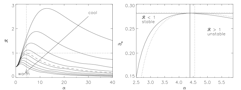
Figure 48: The left panel shows the response function $\mathcal{R}(\alpha,\tilde{\sigma}_{u})$ for axisymmetric disturbances in the $\beta=0.25$ disk. $\mathcal{R}$ is plotted as a function of wavenumber $\alpha$ for different values of the velocity dispersion $\tilde{\sigma}_{u}$. The dashed line is the curve with $\tilde{\sigma}_{u}=\tilde{\sigma}_{u,\min}$, that is, the critical velocity dispersion for stability according to local theory. The right panel shows the marginal stability curve $\mathcal{R}=1$ for the $\beta=0.25$ disk. The solid (dotted) lines indicate the result of the global (local) theory. [The temperature and wavenumber at which instability sets in are marked. These are $\tilde{\sigma}_{u,\min}=0.281$ for global stability, $\tilde{\sigma}_{u,\min}=0.283$ for local stability; $\alpha_{\text{u}}=4.38$ for global stability, $\alpha_{\text{u}}=4.55$ for local stability].

Figure 50: Minimum temperature of the self-consistent power-law disk for global axisymmetric stability plotted against rotation curve index $\beta$. In the left-hand plot, this is presented as the minimum velocity dispersion $\tilde{\sigma}_{u}$, and in the right-hand plot as the stability parameter $Q_{\text{s}}$ necessary to stabilise the disk to axisymmetric perturbations. The dotted line shows the minimum temperature as given by local stability.

6.2 Neutral modes

For the self-consistent disks, the neutral modes must have not just $s=0$ but $\Omega_{\text{p}}=0$ as well. As noted by Lynden-Bell & Lemos (1993), the neutral modes are pure logarithmic spirals. In this case, the transfer function, which describes how the self-consistent disk responds to forcing, can be streamlined from the cumbersome expression given in Section 3.3 of Paper I to a simple delta-function. Let us write $\mathcal{S}_{m}(\alpha,\alpha^{\prime})=\mathcal{R}\delta(\alpha-\alpha^{\prime})$, where $\mathcal{R}$ defines the response function. We derive helpful expressions for the response function in Appendix C and apply these formulae in the following two sub-sections that study the axisymmetric and bisymmetric neutral modes.

6.2.1 Axisymmetric Neutral Modes

The only growing modes admitted by the self-consistent disk are axisymmetric ones. These set in through the neutral modes (Lynden-Bell & Ostriker 1967; Kalnajs 1971). The form of the response function  (C9) in this instance is shown in the left panel of Fig. 48. Now, breathing modes are long wavelength instabilities with no radial nodes. If present, the response function crosses the self-consistent line $\mathcal{R}=1$ as $\alpha\rightarrow 0$. Fig. 48 immediately makes clear that the stellar power-law disks do not admit breathing modes – in contradistinction to the gas power-law disk [Lemos et al. 1991]. Breathing modes are analogous to the instability of stars with $\gamma<4/3$, where $\gamma$ is the ratio of the heat capacity at constant pressure to the heat capacity at constant volume (see Binney & Tremaine 1987, chap. 5). Breathing modes occur in gas disks because gas molecules have internal degrees of freedom, which absorb energy released in changes such as contraction. This energy is then not available to the translational degrees of freedom which contribute to the pressure. There is thus insufficient pressure to resist gravitational collapse. Conversely, when a stellar disk contracts, all the energy released contributes to increased random velocity, which tends to counteract the effect of the increased gravity. Thus stellar disks are much more stable than gas disks to breathing modes.

The marginal stability curve $\mathcal{R}=1$ is plotted in the plane of dimensionless wavenumber $\alpha$ and velocity dispersion $\tilde{\sigma}_{u}$ in the right panel of Fig. 48. This compares the marginal stability curves obtained using local theory (dotted lines) and global theory (solid lines). The agreement is very good, especially close to the critical temperature. Fig. 50 shows the minimum temperature needed for axisymmetric stability both in terms of the velocity dispersion and the stability parameter $Q_{\text{s}}$. It is clear in this plot that the local and global results coincide most closely at $\beta=0$, where the rotation curve is flat. This is probably because Toomre’s local analysis assumes that the stellar disk has a Maxwellian velocity distribution. This is an excellent approximation for the Toomre-Zang disks, less good for the other power-law disks. Local theory becomes discrepant only when $\beta\lesssim-0.25$. Toomre’s (1964) local analysis assumes that the velocity dispersion is small compared to the circular velocity, and that the wavelength of any disturbance is small compared to the radius $R$ at the point under consideration. In the present notation, these conditions are $\tilde{\sigma}_{u}\ll 1$ and $\alpha\gg 1$. They become harder to justify when $\beta<-0.25$. As $\beta$ becomes more negative, the wavelength of the unstable perturbation becomes larger, undermining local theory. The local calculation then underestimates the velocity dispersion needed for axisymmetric stability. Power-law disks with rising rotation curves remain globally unstable even when they are hot enough to be locally stable.

Figure 52: The response function for $m=2$ neutral modes in the self-consistent disks with $\beta=\pm 0.25$. [For $\beta=0.25$, curves are shown for ten values of $Q_{\text{s}}$ in steps of 0.1 from 0.3 to 1.2. For $\beta=-0.25$, curves are shown for seven values of $Q_{\text{s}}$ in steps of 0.1 from 0.3 to 0.9].

6.2.2 Other Neutral Modes

Let us close with a brief examination of the bisymmetric neutral modes admitted by the self-consistent disk. The response function $\mathcal{R}$ for these modes is given by eq. (C6). Fig. 52 shows the dependence of the response function on the wavenumber $\alpha$ for different temperatures. It is difficult to obtain an accurate value for $\mathcal{R}$ when both temperature and wavenumber are high. In Fig. 52, the curve for each temperature has been truncated when the inaccuracy becomes severe enough to be visible on the graph. When the temperature is low enough, the disk admits neutral $m=2$ modes. As the disk is heated, the $\mathcal{R}$-$\alpha$ curve drops, until a critical temperature is reached at which $\mathcal{R}=1$ only at some wavenumber. Above this temperature, the response remains less than unity for all wavenumbers and there are no neutral modes. Fig. 52 demonstrates that disks with falling rotation curves admit neutral modes at higher values of the stability criterion $Q_{\text{s}}$ than disks with rising curves. For $\beta=0.25$, the curve with $Q_{\text{s}}=0.4$ intersects the line $\mathcal{R}=1$, whereas for $\beta=-0.25$, this curve never reaches $\mathcal{R}=1$. The dependence of the critical temperature for neutral modes on $\beta$ is shown in Fig. 54. It has the opposite behaviour to marginally-stable modes in the cut-out disks, which are shown on the same plot.

Figure 54: Velocity dispersion $\tilde{\sigma}_{u}$ and stability parameter $Q_{\text{s}}$ plotted against rotation curve index $\beta$ for an $m=2$ modes in self-consistent and cut-out disks. The curves labelled with the inner cut-out index $N$ show the $\tilde{\sigma}_{u,\min}$ and $Q_{\text{s}}$ at which the inner cut-out disks are marginally stable to bisymmetric disturbances. The curve labelled “scale-free” shows the $\tilde{\sigma}_{u,\min}$ and $Q_{\text{s}}$ at which the self-consistent disk just fails to admit any bisymmetric neutral modes.

7 Conclusions

The work in this paper concludes a linear normal mode analysis of a family of self-gravitating, differentially rotating stellar dynamical disks in which the circular velocity varies as a power of the Galactocentric radius, i.e., $v_{\text{circ}}\propto R^{-\beta/2}$. Our analysis includes both self-consistent disks, in which the surface density and the potential are related through Poisson’s equation, and cut-out disks, in which stars close to the centre (and sometimes also at large radii) are carved out. The analytic and numerical procedures have exploited the self-similar force field of the models to develop a fast code that finds the pattern speeds and growth rates of the normal modes. Some tables of the fastest growing modes are provided in Appendix D. A comparison of these linear stability results with modes as detected in N-body simulations is a worthwhile and interesting task.

(1) The inner cut-out is crucial in allowing growing non-axisymmetric modes in the power-law disks. Physically, it is helpful to picture the instabilities as standing wave patterns caused by the interference of travelling waves in a resonant cavity. For $m>1$, the inner Lindblad resonance absorbs incident waves and damps any disturbance. Growing modes have pattern speeds which are large enough to push the inner Lindblad resonance within the shield of the inner cut-out. Waves cannot propagate easily within the core where there is little active mass. The inner cut-out acts as a reflective barrier. So, it has a destabilising effect if it shields waves from the absorbing inner Lindblad resonance. The inner cut-out is most effective as a reflector of waves when it is abrupt. Disks with lower cut-out indices allow more of the waves to seep through to the resonance and are thus more securely stable. The $N=1$ disk has the mildest cut-out and is the most stable of all.

(2) The stability to different harmonics is summarised in Fig. 56, which shows the minimum velocity dispersion needed for global stability. For an inner cut-out index $N<3$, the disks are more stable to bar-like or bisymmetric modes than to axisymmetric disturbances, whereas for $N>3$, the converse is true. Modes with $m=3$ and $m=4$ are always very hard to excite. The disks must be extremely cold before they admit growing modes with more than two arms.

Figure 56: Minimum temperature for global stability to modes with different azimuthal symmetry.

The most serious instabilities to which all the cut-out disks are susceptible are one-armed instabilities. At outset, let us concede that our analysis permits the $m=1$ modes to shift the barycentre of the galaxy (c.f. Zang 1976). This artefact arises from the rigid core which has been carved out of the galaxy. A full treatment should allow the core to move in response to the growing mode in such a way as to cancel the shifting of the barycentre. Nonetheless, we do not believe this to be a serious flaw – first, because the barycentre moves only slightly within the linear régime and second, because N-body simulations by [Earn 1993], using the code described in [Earn & Sellwood 1995], appear to corroborate the conclusion that one-armed instabilities are the most serious. The prevalence of the one-armed modes can be easily understood at a simple level, as there is no inner Lindblad resonance for $m=1$. This removes a powerful stabilising influence.

What is the physical mechanism generating these one-armed modes? They are not akin to the edge modes [Erickson 1974, Toomre 1981, Sellwood 1989]. There is typically only one edge mode characterised by a single growth rate and pattern speed. By contrast, the cut-out disks exhibit an embarrassingly large number of different one-armed unstable modes. Second, the one-armed modes are not generated by refraction of short trailing waves into long trailing waves (the ‘WASER’) even though the $Q$ profile of the cut-out disks does rise steeply in the inner regions in the manner envisaged by Lin and co-workers [Mark 1976, Lau et al. 1976]. A third possibility, suggested to us by Sellwood (1997, private communication), is that the cut-out may be essentially invisible to long-wavelength disturbances, thus allowing trailing waves to leak through the centre and emerge as leading waves with devastating consequences. This does not seem to be the case, as the dominant wavelengths of the unstable modes are not large compared to the cut-out radius. Rather, the numerical evidence particularly of Fig. 22 seems to us to suggest that the trailing waves are reflected as leading waves at the inner cut-out. It is this that completes the feedback for the swing-amplifier and causes one-armed mayhem in the disk.

(3) For all azimuthal wavenumbers, the unstable modes persist to higher temperatures and grow more vigorously if the rotation curve of the power-law disk is rising ($\beta<0$) rather than falling ($\beta>0$). One way of understanding this result is to recall that, even in local axisymmetric theory, the power-law disks with rising rotation curves are more susceptible to Jeans instabilities and their ilk. In the absence of pressure, they remain vulnerable at longer lengthscales. They require larger velocity dispersions (relative to the local circular speed) for stabilisation at short scales. For example, on moving from $\beta=0.5$ to $\beta=-0.5$, the typical densities increase by a factor of roughly three (c.f., Table 1) and this in itself indicates that instabilities of whatever sort are much more worrisome in the models with rising rotation curves ($\beta<0$). A number of authors [Lovelace & Hohlfield 1978, Papaloizou & Savonjie 1991, Collett 1995] have pointed out that gradients and especially turning points in the ratio of vorticity to surface density (or potential vorticity $\zeta$) can provoke instabilities. In the power-law disks, the potential vorticity behaves like

$$\zeta={\Omega\over\Sigma}\sim R^{-\beta/2}.$$ (16)

The gradient of the potential vorticity actually vanishes in the Toomre-Zang disk ($\beta=0$). In the more nearly Keplerian disks ($\beta>0$), swing amplification is boosted by this effect. In the more nearly uniformly-rotating disks ($\beta<0$), swing amplification gets weakened. Somewhat surprisingly, the effect of gradient terms in the potential vorticity actually runs contrary to the numerical stability results. Any effect, though present, must be quite weak. This has been demonstrated by Alar Toomre in unpublished work.

(4) The criterion suggested by Ostriker and Peebles (1973) for stability against bar-like modes is untrustworthy. It gravely overestimates the energy in the form of random motions necessary to achieve stability against bisymmetric distortions. The power-law disks are much more stable than the criterion suggests. Similar qualms have already been reported by others [Aoki et al. 1979, Toomre 1981].

(5) There are no length-scales and time-scales in the scale-free disks. If any mode is admitted at some pattern speed and growth rate, then it must be present at all pattern speeds and growth rates. Here, the analysis falls short of a complete proof, but our belief is that such a two-dimensional continuum of non-axisymmetric modes does not exist. The weight of the evidence suggests that there is no continuum and that the self-consistent disks admit no growing non-axisymmetric modes whatsoever. There are two telling pieces of evidence in favour of this conclusion. The first is the non-Hermitian nature of the kernel in the Fredholm integral equation for non-axisymmetric modes, which coerces us into satisfying (if we can) two simultaneous integral equations with only one free parameter at our disposal. Second, the behaviour of the mathematical eigenvalues of the cut-out disks in the limit of vanishing pattern speed must mimic that of the self-consistent disks and it does not suggest in the slightest the existence of a continuum modes. At first sight, this conclusion is astonishing – as it applies even to the completely cold disk! But, without reflecting boundaries such as provided by the cut-outs, there is no resonant cavity and no possibility of unstable normal modes. Such an outcome is already familiar in the theory of gaseous accretion disks [Papaloizou & Savonjie 1989, Papaloizou & Lin 1995].

The case of the axisymmetric modes is somewhat different. Now, the kernel is Hermitian and the eigenvalues must be real and positive. There is only one integral equation to be solved with our single disposable parameter. The temperature marking the onset of the neutral modes is accurately given by local theory. On physical grounds, these neutral modes are followed by growing modes as the temperature of the disk is lowered further. But the self-similar disk cannot distinguish between modes with different growth rates. Below the critical temperature the self-consistent disks must admit a one-dimensional continuum of growing axisymmetric modes.

(6) The local theory of Toomre (1964) gives an excellent description of the global axisymmetric stability of the cut-out and the self-consistent power-law disks. The only possible axisymmetric modes are Jeans modes. Breathing modes do not occur in the stellar power-law disks, although they do occur in the gas disks [Lemos et al. 1991]. This is because gas molecules have internal degrees of freedom which can absorb energy released in contraction. This energy is not available to the translational degrees of freedom and does not contribute to the gas pressure resisting collapse. By contrast, when a stellar disk contracts, all the energy released is converted to random motions.

(7) Both the self-consistent and the cut-out disks admit neutral modes. For the self-consistent disks, any neutral modes must have not just $s=0$ but also $\Omega_{\text{p}}=0$. The existence of neutral modes seems to be related to the absence of $m$-lobed closed orbits in the frame rotating with pattern speed $\Omega_{\text{p}}$. The cleanest example of this occurs for neutral triskele modes in the cut-out and self-consistent disks. For such disks with $\beta\leq-0.25$, there are neutral $m=3$, $\Omega_{\text{p}}=0$ modes independent of temperature. These are the very disks for which three-lobed orbits closed in the inertial frame do not occur. This is straightforward to understand. The existence of any three-lobed closed orbits in the $\Omega_{\text{p}}=0$ frame would cause any neutral pattern to evolve.

NWE and JCAR are particularly indebted to David Earn and Jerry Sellwood for the loan of computer code that simulates the evolution of the cut-out power-law disks using the smooth-field-particle code described in David Earn’s Ph. D. thesis. In particular, David Earn kindly re-ran some of the models in his thesis so that the dominant unstable modes could be checked against our linear stability code. We wish to acknowledge valuable conversations with James Binney, Jim Collett, David Earn, Jeremy Goodman, Donald Lynden-Bell, Jerry Sellwood, Alar Toomre and Scott Tremaine – all of whose insights have benefitted us enormously. Both Jerry Sellwood and Alar Toomre offerred extensive and useful comments on earlier versions of the manuscript. Finally, NWE and JCAR thank the Royal Society and the Particle Physics and Astronomy Research Council respectively for financial support.

A Axisymmetric Stability

This appendix briefly discusses the global stability of the cut-out power-law disks to axisymmetric modes. In the axisymmetric case, the marginal modes demarking the boundary between stability and instability are those of zero growth rate and pattern speed [Lynden-Bell & Ostriker 1967, Kalnajs 1971]. In fact, the limit of vanishing growth rate gives rise to some numerical delicacies in the calculation of the kernel of the Fredholm integral equation. The expression for the cut-out angular momentum function $F_{lm}$ is derived in Appendix C of Paper I. For $m=0$, it becomes

$$\lim_{\tilde{s}\rightarrow 0^{+}}F_{l0}(\eta\not=0)=-\frac{2-\beta}{2+\beta}\left|\frac{2+2\gamma-\beta\gamma}{\beta\tilde{U}^{2}+\beta-2}\right|\frac{i}{1-e^{2\pi\hat{\eta}}}\left\{\lim_{\tilde{s}\rightarrow 0^{+}}e^{-i\hat{\eta}\ln\frac{l\tilde{\kappa}}{i\tilde{s}}}+\frac{(1-e^{\pi\hat{\eta}})}{N(1-e^{-\pi\hat{\eta}/N})}\right\}.$$ (A1)

Taking the principal value of the logarithm, we find that

$$\ln{{l\tilde{\kappa}}\over{i\tilde{s}}}=\ln\left|{{l\tilde{\kappa}}\over\tilde{s}}\right|+i\pi\left(1+\text{sign}(l)\times{{1\over 2}}\right),$$ (A2)

and hence the limit in (A1) is

$$\lim_{\tilde{s}\rightarrow 0^{+}}e^{-i\hat{\eta}\ln\frac{l\tilde{\kappa}}{i\tilde{s}}}=e^{\pi\hat{\eta}(1+\text{sign}(l)\times{{1\over 2}})}\lim_{\tilde{s}\rightarrow 0^{+}}e^{-i\hat{\eta}\ln|l\tilde{\kappa}/\tilde{s}|},$$ (A3)

Figure A2: Dependence of the largest mathematical eigenvalue on growth rate $s$ and temperature $Q_{\text{s}}$ for axisymmetric disturbances in inner cut-out disks with $N=2$. [Curves are drawn for six different values of $Q_{\text{s}}$: $Q_{\text{s}}=0.6$, 0.8, 1.0, 1.2, 1.4, 1.6. The $Q_{\text{s}}=1$ curve is drawn with a bolder line. For the $\beta=0.25$ disk, $Q_{\text{s}}=1$ corresponds to a velocity dispersion of $\tilde{\sigma}_{u}=0.283$, and for $\beta=-0.25$, to $\tilde{\sigma}_{u}=0.509$].

For very negative values of $\eta$, the $e^{\pi\eta}$ term in (A3) ensures that the limit is zero. But for positive $\eta$, the expression for $F_{lm}$ fails to converge to any definite limit. This might be expected to present problems for the numerical implementation. Fortunately, it turns out that the mathematical eigenvalue converges even though $F_{lm}$ does not (see Read 1997 for ample numerical evidence). This is because – especially when the growth rate is small – the eigenvalue is dominated by the matrix elements along the diagonal $\eta=0$, where the troublesome term is simply unity. In eq. (A1), we can write $N(1-e^{-\pi\hat{\eta}/N})\approx\pi\hat{\eta}$ close to $\eta=0$. The dependence on the inner cut-out function $N$ is cancelled out in the matrix elements close to the diagonal, where the transfer function is largest. We thus expect the stability of the inner cut-out disk to be virtually independent of $N$ – as already argued on physical grounds.

Fig. A2 shows how the mathematical eigenvalue depends on growth rate and temperature for two sample cut-out disks. For sufficiently small $Q_{\text{s}}$, a unit eigenvalue can always be found for large enough growth rate $s$. When the disk is cool, it is susceptible to fiercely growing modes. As the disk is heated, the growth rate of the unstable mode decreases. The temperature at which the disk is marginally stable is given by the $Q_{\text{s}}$ for which the $s=0^{+}$ eigenvalue is unity. Inspection of Fig. A2 shows that this value of $Q_{\text{s}}$ is close to unity. This already suggests that the global axisymmetric stability of the cut-out disks is close to the local axisymmetric stability. Fig. A4 shows the velocity dispersion $\tilde{\sigma}_{u,\min}$ and the stability parameter $Q_{\text{s}}$ of the marginally stable disks as a function of rotation curve index $\beta$. Four different values of $N$ are plotted, but the curves are scarcely distinguishable. For comparison, the results of local theory for the self-consistent disk are shown in a dotted line.

Figure A4: Minimum temperature for global axisymmetric stability plotted against rotation curve index $\beta$ for disks with various cut-out functions. The left panel shows the minimum velocity dispersion $\tilde{\sigma}_{u}$; the right panel shows the same data in terms of the stability parameter $Q_{\text{s}}$. The dotted lines show the local theory; other lines indicate results of global theory for an inner cut-out disks. [Results for $N=1$, 2, 3, 4 are plotted in both graphs, but coincide so closely as to be virtually indistinguishable.]

Local theory is an excellent guide to the global stability of the inner cut-out disks. This is in accordance with Toomre and Zang’s findings – for the disk with a flat rotation curve, local and global results agree “to within a few tenths of one per cent” [Zang 1976]. The value of the inner cut-out index has little effect on the stability. An additional outer cut-out function tends to make the disk slightly more stable, in that a lower velocity dispersion is needed for axisymmetric stability.

B The Symmetry of the Self-Consistent Disk

In this appendix, we demonstrate that if any modes with $\omega\neq 0$ exist in the self-consistent disk, then they must form a two-dimensional continuum. This proof is a straightforward extension of that due to Kalnajs in 1974 for the disk with a flat rotation curve (given in Zang’s (1976) thesis).

For the scale-free disk, the angular momentum function is defined as

$$F_{lm}(\eta)=\left\{(l\tilde{\kappa}+m\tilde{\Omega})\left|\frac{2+2\gamma-\beta\gamma}{\beta\tilde{U}^{2}+\beta-2}\right|-\gamma m\right\}{1\over{2\pi}}\int_{0}^{\infty}{{e^{-i\eta{2\over{2-\beta}}\ln\tilde{L}_{z}}}\over{l\tilde{\kappa}+m\tilde{\Omega}-\tilde{\omega}\tilde{L}_{z}^{\frac{2+\beta}{2-\beta}}}}{{d\tilde{L}_{z}}\over\tilde{L}_{z}}.$$ (B1)

where the notation of Paper I is used. As shown in Appendix C of Paper I, the angular momentum function consists of a regular function and a Dirac delta-function. Here, let us write:

$$F_{lm}(\eta)=F_{lm}^{(1)}(\eta)+F_{lm}^{(2)}\delta(\eta)$$ (B2)

where

$$F_{lm}^{(1)}(\eta)=-\frac{2-\beta}{2+\beta}\left\{\left|\frac{2+2\gamma-\beta\gamma}{\beta\tilde{U}^{2}+\beta-2}\right|-\frac{\gamma m}{l\tilde{\kappa}+m\tilde{\Omega}}\right\}\frac{ie^{-i\hat{\eta}\ln{l\tilde{\kappa}+m\tilde{\Omega}\over\tilde{\omega}}}}{1-e^{2\pi\hat{\eta}}},$$ (B3)

$$F_{lm}^{(2)}=\frac{2-\beta}{4}\left\{\left|\frac{2+2\gamma-\beta\gamma}{\beta\tilde{U}^{2}+\beta-2}\right|-\frac{\gamma m}{l\tilde{\kappa}+m\tilde{\Omega}}\right\},$$ (B4)

and $\hat{\eta}=2\eta/(2+\beta)$. (For $m\neq 0$, these expressions hold for all $l$. For $m=0$, there is an ambiguity at the $l=0$ harmonic. The correct choices are $F_{00}^{(1)}=F_{00}^{(2)}=0$). When $\omega=0$, the angular momentum function is simply a delta-function in $\eta$:

$$F_{lm}(\eta)=\left\{\left|\frac{2+2\gamma-\beta\gamma}{\beta\tilde{U}^{2}+\beta-2}\right|-\frac{\gamma m}{l\tilde{\kappa}+m\tilde{\Omega}}\right\}\int_{0}^{\infty}\frac{e^{-i\eta{2\over{2-\beta}}\ln\tilde{L}_{z}}}{2\pi}{{d\tilde{L}_{z}}\over\tilde{L}_{z}}=\frac{2-\beta}{2}\left\{\left|\frac{2+2\gamma-\beta\gamma}{\beta\tilde{U}^{2}+\beta-2}\right|-\frac{\gamma m}{l\tilde{\kappa}+m\tilde{\Omega}}\right\}\delta(\eta).$$ (B5)

When $\omega=0$, we do not pick up the “off-diagonal” terms describing the response at wavelengths different from that of the original perturbation. Let us note that $F_{lm}^{(1)}(\eta)$ has no unique limiting value as $\omega\rightarrow 0$. It does not tend to zero in this limit and the case $\omega=0$ cannot be recovered by taking the limit $\omega\rightarrow 0$. Physically, this is a consequence of the symmetry of the disk. A pure logarithmic spiral is self-similar and a neutral logarithmic spiral introduces no length- or time-scales through its growth rate and pattern speed. Thus the response must be purely self-similar, i.e., another logarithmic spiral. Once the logarithmic spiral is allowed to grow or rotate – however slowly – a length- and time-scale has been introduced. The response is no longer self-similar, but involves contributions at many wavelengths.

Analogously to (B2), let us divide the transfer function into a regular part and a Dirac delta-function:

$$\mathcal{S}_{m}(\alpha,\alpha^{\prime})=\mathcal{S}_{m}^{(1)}(\alpha,\alpha^{\prime})+\delta(\alpha-\alpha^{\prime})\mathcal{S}_{m}^{(2)}(\alpha,\alpha^{\prime}).$$ (B6)

$\mathcal{S}_{m}^{(1)}(\alpha,\alpha^{\prime})$ and $\mathcal{S}_{m}^{(2)}(\alpha,\alpha^{\prime})$ may be obtained from eq. (78) of Paper I, using $F_{lm}^{(1)}$ and $F_{lm}^{(2)}$ respectively in place of $F_{lm}$. We see that $F_{lm}^{(1)}(\eta)$ admits the factorisation

$$F_{lm}^{(1)}(\eta)=e^{i\hat{\eta}\ln\tilde{\omega}}\hat{F}_{lm}^{(1)}(\eta),.$$ (B7)

where $\hat{F}_{lm}^{(1)}(\eta)$ is independent of the growth rate and pattern speed. The transfer function depends on the growth rate only through the angular momentum function. So, $\mathcal{S}_{m}^{(2)}(\alpha,\alpha^{\prime})$ is independent of $\tilde{\omega}$, while the dependence of $\mathcal{S}_{m}^{(1)}(\alpha,\alpha^{\prime})$ on $\tilde{\omega}$ can be factorised out as

$$\mathcal{S}_{m}^{(1)}(\alpha,\alpha^{\prime})=e^{i(\hat{\alpha}-\hat{\alpha}^{\prime})\ln\tilde{\omega}}\hat{\mathcal{S}}_{m}^{(1)}(\alpha,\alpha^{\prime}),$$ (B8)

where $\hat{\alpha}$ is defined by $\hat{\alpha}=2\alpha/(2+\beta)$ and $\hat{\mathcal{S}}_{m}^{(1)}(\alpha,\alpha^{\prime})$ is independent of $\tilde{\omega}$. Let us define reduced transforms via:

$$\hat{A}(\alpha)=e^{-i\hat{\alpha}\ln\tilde{\omega}}A(\alpha).$$ (B9)

Then, the Fredholm integral equation becomes

$$\lambda\hat{A}(\alpha)=\hat{A}(\alpha)\mathcal{S}_{m}^{(2)}(\alpha,\alpha)+\int_{-\infty}^{+\infty}d\alpha^{\prime}\hat{A}(\alpha^{\prime})\hat{\mathcal{S}}_{m}^{(1)}(\alpha,\alpha^{\prime}),$$ (B10)

where none of the quantities depend on $\tilde{\omega}$. This means that if a non-trivial solution $\hat{A}(\alpha)$ exists at all, then self-consistent modes $A(\alpha)$ exist with any non-vanishing growth rate and pattern speed.

C Neutral Modes of the Self-Consistent Disk

In this appendix, expressions are derived for the response of the self-consistent disk to elementary forcing by a pure logarithmic spiral. For the neutral modes, the angular momentum function is simply a delta-function (B5). Thus, the transfer function is also proportional to a delta-function. Let us write $\mathcal{S}_{m}(\alpha,\alpha^{\prime})=\mathcal{R}\delta(\alpha-\alpha^{\prime})$, where $\mathcal{R}$ is the response function:

$$\begin{split}\mathcal{R}&=\left(1-\frac{\beta}{2}\right)2\pi GK(\alpha,m)\tilde{C}R_{0}^{\gamma+1}v_{\beta}^{{2\over\beta}(1+\gamma)}\int d\tilde{U}\,\mathcal{J}_{0}(\tilde{U})\tilde{U}\\ &\times\left|\frac{\beta\tilde{U}^{2}+\beta-2}{2\beta}\right|^{{1\over\beta}+{\gamma\over\beta}-{\gamma\over 2}}\sum_{l=-\infty}^{+\infty}|Q_{lm}(\alpha)|^{2}\left\{\left|\frac{2+2\gamma-\beta\gamma}{\beta\tilde{U}^{2}+\beta-2}\right|-\frac{\gamma m}{l\tilde{\kappa}+m\tilde{\Omega}}\right\}.\end{split}$$ (C1)

The response density transform $A_{\text{res}}(\alpha)$ at any wavenumber $\alpha$ is simply proportional to the imposed density transform $A_{\text{imp}}(\alpha)$. Physically, the ratio of the response density to the imposed perturbation is given by the response function $\mathcal{R}$. If $\mathcal{R}>1$, the perturbation grows; if $\mathcal{R}<1$, the perturbation dies away. Self-consistent neutral modes require $\mathcal{R}=1$. We note that $\mathcal{R}$ is real and independent of the radial position in the disk, so that the disk is either stable or unstable everywhere. Recalling the symmetry properties of the Kalnajs function and of the Fourier coefficients, it is evident that the response function is independent of the sign of the wavenumber. This is an expression of the anti-spiral theorem [Lynden-Bell & Ostriker 1967]. Every spiral of wavenumber $\alpha$ comes with an “anti-spiral” of wavenumber $-\alpha$. Hence any neutral modes come in pairs, one leading and one trailing.

There is an alternative form of the response function (C1), which merely involves integration over one period of the unperturbed orbit. This is especially useful for the important case of the $m=0$ neutral modes, as it resolves the ambiguity at the $l=0$ harmonic. In this derivation, the response to a pure logarithmic spiral is itself assumed to be a pure logarithmic spiral. According to Zang (1976), this calculation was carried out for the axisymmetric neutral modes of the disk with a completely flat rotation curve by Toomre in the 1960s. Putting together eqs. (51), (58) and (68) of Paper I, we obtain for the change in the distribution function

$$f_{\text{imp}}(t)=\tilde{C}L_{z}^{\gamma-1}|E|^{\frac{1}{\beta}+\frac{\gamma}{\beta}-\frac{\gamma}{2}}\psi_{\text{imp}}^{\alpha m}(t)\left\{\left|\frac{1}{\beta}+\frac{\gamma}{\beta}-\frac{\gamma}{2}\right|\frac{L_{z}}{|E|}+i\left(\left|\frac{1}{\beta}+\frac{\gamma}{\beta}-\frac{\gamma}{2}\right|\frac{L_{z}}{|E|}\omega-m\gamma\right)\int_{-\infty}^{t}\frac{\psi_{\text{imp}}^{\alpha m}\left(t^{\prime}\right)}{\psi_{\text{imp}}^{\alpha m}(t)}dt^{\prime}.\right\}$$ (C2)

Substituting the potential of a single logarithmic spiral, we obtain

$$\begin{split}&f_{\text{imp}}(t)=2\pi G\tilde{C}\Sigma_{\text{p}}K(\alpha,m)R_{0}L_{z}^{\gamma-1}\left|E\right|^{1/\beta+\gamma/\beta-\gamma/2}e^{i\left(m\theta-\omega t\right)}\left({R\over{R_{0}}}\right)^{i\alpha-{{1\over 2}}}\left\{\left|\frac{1}{\beta}+\frac{\gamma}{\beta}-\frac{\gamma}{2}\right|\frac{L_{z}}{|E|}\right.\\ &\left.+i\left(\left|\frac{1}{\beta}+\frac{\gamma}{\beta}-\frac{\gamma}{2}\right|\frac{L_{z}}{|E|}\omega-m\gamma\right)\int_{-\infty}^{t}e^{i\left(m(\theta^{\prime}-\theta)-\omega(t^{\prime}-t)\right)}\left({R^{\prime}\over{R}}\right)^{i\alpha-{{1\over 2}}}dt^{\prime}\right\}.\end{split}$$ (C3)

The integral in this equation can be split up into an infinite sequence of integrals over the radial period $T$. Summing the geometric progression, we have

$$\begin{split}&f_{\text{imp}}(t)=2\pi G\tilde{C}\Sigma_{\text{p}}K(\alpha,m)R_{0}L_{z}^{\gamma-1}|E|^{1/\beta+\gamma/\beta-\gamma/2}e^{i\left(m\theta-\omega t\right)}\left({R\over{R_{0}}}\right)^{i\alpha-{{1\over 2}}}\left\{\left|\frac{1}{\beta}+\frac{\gamma}{\beta}-\frac{\gamma}{2}\right|\frac{L_{z}}{|E|}\right.\\ &\left.+i\left(\left|\frac{1}{\beta}+\frac{\gamma}{\beta}-\frac{\gamma}{2}\right|\frac{L_{z}}{|E|}\omega-m\gamma\right)\frac{1}{1-e^{-iT(m\Omega-\omega)}}\int_{t-T}^{t}e^{i\left(m(\theta^{\prime}-\theta)-\omega(t^{\prime}-t)\right)}\left({R^{\prime}\over{R}}\right)^{i\alpha-{{1\over 2}}}dt^{\prime}\right\}.\end{split}$$ (C4)

For $m\neq 0$, we simply set $\omega=0$ to obtain

$$\begin{split}f_{\text{imp}}(t)&=2\pi G\tilde{C}\Sigma_{\text{p}}K(\alpha,m)R_{0}L_{z}^{\gamma-1}|E|^{1/\beta+\gamma/\beta-\gamma/2}e^{im\theta}\left({R\over{R_{0}}}\right)^{i\alpha-{{1\over 2}}}\\ &\times\left\{\left|\frac{1}{\beta}+\frac{\gamma}{\beta}-\frac{\gamma}{2}\right|\frac{L_{z}}{|E|}-\frac{im\gamma}{1-e^{-im\Omega T}}\int_{t-T}^{t}e^{im(\theta^{\prime}-\theta)}\left({R^{\prime}\over{R}}\right)^{i\alpha-{{1\over 2}}}dt^{\prime}\right\}.\end{split}$$ (C5)

This expression can then be integrated over velocity space to obtain the response density $\Sigma_{\text{res}}$. Recalling the definition of the response function $\mathcal{R}$, we finally obtain

$$\begin{split}\mathcal{R}&=2\pi G\tilde{C}K(\alpha,m)R\iint du\,dv\,L_{z}^{\gamma-1}|E|^{1/\beta+\gamma/\beta-\gamma/2}\\ &\times\left\{\left|\frac{1}{\beta}+\frac{\gamma}{\beta}-\frac{\gamma}{2}\right|\frac{L_{z}}{|E|}-\frac{im\gamma}{1-e^{-im\Omega T}}\int_{t-T}^{t}e^{im(\theta^{\prime}-\theta)}\left({R^{\prime}\over{R}}\right)^{i\alpha-{{1\over 2}}}dt^{\prime}\right\}.\end{split}$$ (C6)

This expression can be shown to be equivalent to that obtained directly from the Fredholm integral equation (see Read 1997).

When the imposed perturbation is axisymmetric, eq. (C4) is singular, viz.,

$$\begin{split}f_{\text{imp}}(t)&=2\pi GK(\alpha,0)\tilde{C}\Sigma_{\text{p}}R_{0}e^{st}\left({R\over{R_{0}}}\right)^{i\alpha-{{1\over 2}}}L_{z}^{\gamma-1}|E|^{1/\beta+\gamma/\beta-\gamma/2}\\ &\times\left\{\left|\frac{1}{\beta}+\frac{\gamma}{\beta}-\frac{\gamma}{2}\right|\frac{L_{z}}{|E|}\right.\left.-\left|\frac{1}{\beta}+\frac{\gamma}{\beta}-\frac{\gamma}{2}\right|\frac{L_{z}}{|E|}\frac{s}{1-e^{-sT}}\int_{t-T}^{t}e^{s(t^{\prime}-t)}\left({R^{\prime}\over{R}}\right)^{i\alpha-{{1\over 2}}}dt^{\prime}\right\}\end{split}$$ (C7)

Using l’Hôpital’s rule to take the limit as $s\rightarrow 0$, we find

$$f_{\text{imp}}(t)=2\pi GK(\alpha,0)\tilde{C}\Sigma_{\text{p}}R_{0}\left|\frac{1}{\beta}+\frac{\gamma}{\beta}-\frac{\gamma}{2}\right|\left({R\over{R_{0}}}\right)^{i\alpha-{{1\over 2}}}L_{z}^{\gamma}|E|^{1/\beta+\gamma/\beta-\gamma/2-1}\left\{1-\frac{1}{T}\int_{t-T}^{t}\left({R^{\prime}\over{R}}\right)^{i\alpha-{{1\over 2}}}dt^{\prime}\right\}.$$ (C8)

This can be integrated over velocity to obtain the axisymmetric response function

$$\mathcal{R}=2\pi GK(\alpha,0)\tilde{C}\left|\frac{1}{\beta}+\frac{\gamma}{\beta}-\frac{\gamma}{2}\right|R\iint du\,dv\,L_{z}^{\gamma}|E|^{1/\beta+\gamma/\beta-\gamma/2-1}\left\{1-\frac{1}{T}\int_{t-T}^{t}\left({R^{\prime}\over{R}}\right)^{i\alpha-{{1\over 2}}}dt^{\prime}\right\}.$$ (C9)

In practice, these forms of the response function for neutral modes are more useful than (C1) because they involve a quadrature performed over just one radial oscillation of the orbit.

D Fastest Growing Modes of the Cut-Out Disks

The following sets of tables compare the stability of inner cut-out disks to perturbations of different azimuthal symmetry $m$. For each symmetry $m$ and inner cut-out index $N$, the pattern speed and growth rate of the fastest-growing mode are recorded. The results for $\beta=0.25$, $\beta=0.00$ and $\beta=-0.25$ are shown in different tables. The numerical accuracy parameters are: $n=301$, $\Delta\alpha=0.1$, $l_{\min}=-30$, $l_{\max}=+40$, $n_{GL}=9$, $f_{\sigma}=0.8$, $a_{\text{acc}}=20$, $b_{\text{acc}}=2$, $\epsilon_{\lambda}=10^{-6}$. The data in the tables are also presented in graphical form in the Figs D1 and D2. The pattern speed of the fastest-growing mode depends almost linearly on $N$. The fastest growth rate increases quite steeply with $N$, reflecting the increased instability of the more sharply cut-out disks.

$Q_{\text{s}}=1.0$, $\beta=0.25$: $\tilde{\sigma}_{u}=0.283$, $\gamma=11.0$
	$m=1$		$m=2$		$m=3$
$N$	$\Omega_{\text{p}}$	$s$	$\Omega_{\text{p}}$	$s$	$\Omega_{\text{p}}$	$s$
1	0.097362	0.014041	-	-	-	-
2	0.157969	0.050158	-	-	-	-
3	0.192207	0.078881	-	-	-	-
4	0.213645	0.099969	0.460196	0.060416	-	-
5	0.228252	0.115400	0.466727	0.128279	-	-
6	0.238798	0.126749	0.472435	0.170714	-	-
7	0.246718	0.135160	0.477593	0.199573	0.619188	0.016944
8	0.252824	0.141454	0.482190	0.220295	0.623895	0.076268

$Q_{\text{s}}=1.0$, $\beta=0.00$: $\tilde{\sigma}_{u}=0.378$, $\gamma=6.00$
	$m=1$		$m=2$		$m=3$
$N$	$\Omega_{\text{p}}$	$s$	$\Omega_{\text{p}}$	$s$	$\Omega_{\text{p}}$	$s$
1	0.085847	0.024053	-	-	-	-
2	0.140888	0.065923	-	-	-	-
3	0.170997	0.096969	0.433518	0.021843	-	-
4	0.189628	0.119035	0.439460	0.127192	-	-
5	0.202258	0.134777	0.445317	0.185191	-	-
6	0.211327	0.146108	0.451135	0.222089	0.600215	0.006528
7	0.218103	0.154365	0.456487	0.247575	0.605870	0.081236
8	0.223301	0.160461	0.461228	0.266062	0.610127	0.134753

$Q_{\text{s}}=1.0$, $\beta=-0.25$: $\tilde{\sigma}_{u}=0.509$, $\gamma=3.36$
	$m=1$		$m=2$		$m=3$
$N$	$\Omega_{\text{p}}$	$s$	$\Omega_{\text{p}}$	$s$	$\Omega_{\text{p}}$	$s$
1	0.080733	0.034289	-	-	-	-
2	0.132275	0.081594	-	-	-	-
3	0.160210	0.115238	0.423391	0.102223	-	-
4	0.177418	0.138674	0.427591	0.191581	-	-
5	0.189107	0.155207	0.433935	0.242558	-	-
6	0.197443	0.166961	0.440325	0.276073	0.599256	0.141945
7	0.203663	0.175475	0.446097	0.299705	0.599256	0.141945
8	0.208430	0.181740	0.451131	0.317072	0.603496	0.190117

Figure D2: The variation of the growth rate and pattern speed of the fastest-growing $m=1$ modes plotted against cut-out index $N$. All disks have $Q_{\text{s}}=1.0$. The solid line marked with diamonds is $\beta=0.25$; the dotted line with triangles is $\beta=0.00$; the dashed line with squares is $\beta=-0.25$.

Figure D4: The variation of the growth rate and the pattern speed of the fastest-growing $m=2$ modes plotted against cut-out index $N$. All disks have $Q_{\text{s}}=1.0$. The solid line marked with diamonds is $\beta=0.25$; the dotted line with triangles is $\beta=0.00$; the dashed line with squares is $\beta=-0.25$.

References

- Aoki et al. 1979 Aoki S., Noguchi M., & Iye M., 1979, PASJ, 31, 737
- Athanassoula & Sellwood 1986 Athanassoula E. & Sellwood J. A., 1986, MNRAS, 221, 213
- Baldwin et al. 1980 Baldwin J. E., Lynden-Bell D., & Sancisi R., 1980, MNRAS, 193, 313
- Bardeen 1978 Bardeen J. M., 1978, in A. Hayli (ed.), Dynamics of Stellar Systems, (IAU Symposium 77), p. 297, Reidel, Dordrecht
- Bertin & Lin 1996 Bertin G. & Lin C. C., 1996, Spiral Structure in Galaxies, MIT Press, Cambridge, Massachussetts
- Collett 1995 Collett J. L., 1995, Ph.D. thesis, Cambridge University, Cambridge
- Earn 1993 Earn D. J. D., 1993, Ph.D. thesis, Cambridge University, Cambridge
- Earn & Sellwood 1995 Earn D. J. D. & Sellwood J. A., 1995, ApJ, 451, 533
- Elmegreen & Elmegreen 1985 Elmegreen D. M. & Elmegreen B. G., 1985, ApJ, 288, 438
- Erickson 1974 Erickson S. A., 1974, Ph.D. thesis, Massachusetts Institute of Technology, Cambridge, Massachusetts
- Evans 1994 Evans N. W., 1994, MNRAS, 267, 333
- Goldreich & Lynden-Bell 1965 Goldreich P. & Lynden-Bell D., 1965, MNRAS, 130, 125
- Gradshteyn & Ryzhik 1978 Gradshteyn I. & Ryzhik I., 1978, Table of Integrals, Series and Products, Academic Press, San Diego
- Hohl 1971 Hohl F., 1971, ApJ, 168, 343
- Kalnajs 1971 Kalnajs A. J., 1971, ApJ, 166, 275
- Kalnajs 1972 Kalnajs A. J., 1972, ApJ, 175, 63
- Kalnajs 1977 Kalnajs A. J., 1977, ApJ, 212, 637
- Kalnajs 1978 Kalnajs A. J., 1978, in E. M. Berkhuisjen & R. Wielebinski (eds.), The Structure and Properties of Nearby Galaxies, (IAU Symposium 77), p. 113, Reidel, Dordrecht
- Lau et al. 1976 Lau Y., Lin C. C., & Mark J. W.-K., 1976, Proc. Nat. Acad. Sci. U.S.A., 73, 1379
- Lemos et al. 1991 Lemos J. P. S., Kalnajs A. J., & Lynden-Bell D., 1991, ApJ, 375, 484
- Lovelace & Hohlfield 1978 Lovelace R. V. E. & Hohlfield R. G., 1978, ApJ, 221, 58
- Lynden-Bell & Lemos 1993 Lynden-Bell D. & Lemos J. P. S., 1993, Equiangular spiral modes of power law disks, unpublished
- Lynden-Bell & Ostriker 1967 Lynden-Bell D. & Ostriker J. P., 1967, MNRAS, 136, 101
- Mark 1976 Mark J. W.-K., 1976, ApJ, 206, 418
- Maxwell 1859 Maxwell J. C., 1859, in W. D. Niven (ed.), The Scientific Papers of James Clerk Maxwell, Dover
- Ostriker & Peebles 1973 Ostriker J. P. & Peebles P. J. E., 1973, ApJ, 186, 467
- Papaloizou & Lin 1995 Papaloizou J. C. B. & Lin D. N. C., 1995, ARAA, 33, 505
- Papaloizou & Savonjie 1989 Papaloizou J. C. B. & Savonjie G. J., 1989, in J. A. Sellwood (ed.), Dynamics of Astrophysical Disks, p. 103, Cambridge University Press, Cambridge
- Papaloizou & Savonjie 1991 Papaloizou J. C. B. & Savonjie G. J., 1991, MNRAS, 248, 353
- Read 1997 Read J. C. A., 1997, Ph.D. thesis, Oxford University, Oxford
- Richter & Sancisi 1994 Richter O.-G. & Sancisi R., 1994, AA, 290, L9
- Rix & Zaritsky 1995 Rix H.-W. & Zaritsky D., 1995, ApJ, 447, 82
- Schmitz & Ebert 1987 Schmitz F. & Ebert R., 1987, A&A, 181, 41
- Sellwood 1989 Sellwood J. A., 1989, in J. A. Sellwood (ed.), Dynamics of Astrophysical Disks, p. 155, Cambridge University Press, Cambridge
- Sellwood & Wilkinson 1993 Sellwood J. A. & Wilkinson A., 1993, Rep. Prog. Phys., 56, 173
- Sparke & Sellwood 1987 Sparke L. & Sellwood J. A., 1987, MNRAS, 225, 653
- Syer & Tremaine 1996 Syer D. & Tremaine S., 1996, MNRAS, 281, 925
- Toomre 1964 Toomre A., 1964, ApJ, 139, 1217
- Toomre 1977 Toomre A., 1977, ARAA, 15, 437
- Toomre 1981 Toomre A., 1981, in S. M. Fall & D. Lynden-Bell (eds.), The Structure and Evolution of Normal Galaxies, p. 111, Cambridge University Press, Cambridge
- Zang 1976 Zang T. A., 1976, Ph.D. thesis, Massachusetts Institute of Technology, Cambridge, Massachusetts