Detecting Scale-Dependence of Bias from APM-BGC Galaxies

Abstract

We present an investigation of the scale-dependence of bias described by the linear model: $(\delta\rho({\bf x})/\bar{\rho})_{g}=b(\delta\rho({\bf x})/\bar{\rho})_{m}$, $b$ being the bias parameter, and $\rho({\bf x})_{g}$ and $\rho({\bf x})_{m}$ are the galaxy number density and mass density, respectively. Using a discrete wavelet decomposition, we show that the behavior of bias scale-dependence cannot be described by one parameter $b$. In the linear bias model the scale-dependence should be measured by the $j$-spectra of wavelet-coefficient-represented bias parameters $\tilde{b}^{(n)}_{j}$ and $b_{j}^{(n)}$, $n$ being positive integers. Because $\tilde{b}^{(n)}_{j}$ with different $n$ are independent from each other, a systematic analysis of the $j$-spectra of $\tilde{b}^{(n)}_{j}$ and $b_{j}^{(n)}$ is necessary.

We performed a $j$-spectrum analysis for samples of elliptical and lenticular (EL), and spiral (SP) galaxies listed in the APM bright galaxy catalog. We found that, for statistics of two-point correlation functions or DWT power spectrum, the scale-independence holds within 1 $\sigma$. However, the bias scale-dependence becomes substantial when phase-sensitive statistics (e.g. $\tilde{b}^{(n)}_{j}$ with $n>2$ or $b_{j}^{(n)}$) are applied. These results indicate that the bias scale-dependence has the same origin as the non-Gaussianity of galaxy distributions. This is generally consistent with the explanation that the bias scale-dependence originated from non-linear and non-local relationship between galaxy formation and their environment.

1 Introduction

Bias is introduced to reconcile the amplitude of fluctuations inferred from clustering of galaxies with that derived from mass distributions. Bright galaxies seem to have a stronger clustering than that of the underlying mass. Therefore, it is generally believed that galaxies are biased tracers of the mass density field, i.e. it follows the clustering of (dark) matter but with an enhanced amplitude.

Generally, bias is phenomenologically modeled by a linear relation as

$$\delta({\bf x})_{g}=b\delta({\bf x})_{m}.$$ (1)

where $\delta({\bf x})_{g}=[n({\bf x})-\bar{n}]/\bar{n}$, $\delta({\bf x})_{m}=[\rho({\bf x})-\bar{\rho}]/\bar{\rho}$, $\rho({\bf x})$ and $n({\bf x})$ are, respectively, the galaxy number density distribution and density field of dark matter, and $\bar{\rho}$ and $\bar{n}$ being the average of $\rho({\bf x})$ and $n({\bf x})$. The phenomenological bias parameter $b$ is assumed to be constant, but may be different for different galaxy types, say, $b_{early}$, $b_{late}$ for early and late types of galaxies.

Eq.(1) and its variants are widely used in the determination of cosmological parameters from samples of redshift surveys of galaxies. However, we have really very little idea about which the bias parameter $b$ should be. In fact, both bias ($b>1$) and anti-bias ($b<1$) are employed in current data analysis (e.g. Mo, Jing & White 1996.) This prevents unambiguous measures of cosmological parameters, giving only bias-contaminated results.

Theoretically, the physical mechanism responsible for relation (1) is far from clear. The first analytic model of bias, in which objects are identified with high peaks or collapsed halos of the density field, offers a plausible explanation of the bias of galaxy clusters – the correlation amplitudes of clusters are strong functions of cluster richness (Kaiser 1984). In this case, bias is mainly caused by the mass of collapsed halos. The larger the mass of the halo, the higher the richness of the cluster.

Yet, the formation of galaxies doesn’t depend only on the mass, or local mass density, of collapsed halos, but is substantially modulated by various environmental effects, such as the suppression of star formation in neighboring protogalaxies (Rees 1985), stimulating the formation of nearby galaxies (Dekel & Rees 1987), dynamical friction effects (Couchman & Carlberg 1992), etc. All these environmental effects are beyond local density, and lead to a non-local relation between the number density of galaxies and the background mass field (Bower et al. 1993). Moreover, the rate of star formation is most likely non-linearly dependent on local mass density. A common result of the non-local and/or non-linear relation between $\delta_{g}$ and $\delta_{m}$ is the scale-dependence of parameter $b$. Therefore, to have a deep understanding of the mechanism of galaxy bias, searching for the scale-dependence of parameter $b$ is necessary (Coles 1993, Catelan et al. 1994.)

So far, the results of detecting $b$ scale-dependence are quite scattered. For instance, the values of the bias-contaminated density parameter $\beta=\Omega^{0.6}/b$ are found to be in the range of 0.4 - 1, and equal to about $\sim 0.5-0.6$ at Gaussian smoothing scales of 3-6 h^-1Mpc, and $\sim 1$ on scales of $\sim 12$ h^-1Mpc (e.g. Dekel, Burstein & White 1996). This is, $b$ is probably scale-dependent from 6 to 12 h^-1 Mpc. On the other hand, some studies conclude that for galaxies of all types and luminosities the scale dependence of the bias parameter is weak (e.g. Kauffmann, Nusser & Steinmetz 1997). Why different detections gave different conclusions? This question motivated us to study the physics included in Eq.(1).

In the first part of this paper, we show that even in linear bias model, the behavior of scale-dependence cannot be described by one parameter $b$, but by a series of $j$-spectra of wavelet-coefficient-represented bias parameters $\tilde{b}^{(n)}_{j}$ and $b_{j}^{(n)}$, $n$ being positive integers. The $j$-spectra of $\tilde{b}^{(n)}_{j}$ are all statistically independent. Different detections may actually measure different parameters $\tilde{b}_{j}^{(n)}$. Therefore, it should not be surprised that some detections are positive, and some negative. The different behavior of bias scale-dependence given by different detection does not cause confusion, but may greatly be helpful to reveal the physics behind the bias model (1). Therefore, to have a complete picture of bias scale-dependence a systematic analysis of the $j$-spectra of $\tilde{b}^{(n)}_{j}$ and $b_{j}^{(n)}$ is necessary.

In the second part, we performed a systematic detection of the bias scale-dependence with the samples of galaxies listed in the APM bright galaxies catalog (APM-BGC). This analysis shows that for the APM-BGC sample, the scale-independence approximately holds if only the two-point correlation function and power spectrum are involved, while the scale-dependence becomes substantial when higher order or phase-sensitive statistics involved. This result is worth to constrain models of hierarchical clustering of galaxies.

The paper is organized as follows. In §2 we briefly introduce a method of the space-scale decomposition based on discrete wavelet transform (DWT) analysis. With this method, various statistics of measuring the bias scale dependence are developed and presented. §3 describes the sample to be analyzed. In §4 we apply the DWT method to analyze the galaxy sample of the APM bright galaxies. The implications of these results are discussed in §5.

2 Linear bias model in DWT representation

2.1 The discrete wavelet transform

Let us briefly introduce the DWT analysis of large scale structures, for the details referring to (Fang & Pando 1997, Pando & Fang 1996, 1998.) We consider here a 1-D mass density distribution $\rho(x)$ or contrast $\delta(x)=[\rho(x)-\bar{\rho}]/\bar{\rho}$, which are mathematically random fields over a spatial range $0\leq x\leq L$. It is not difficult to extend all results developed in this section into 2-D and 3-D because the DWT bases for higher dimension can be constructed by a direct product of 1-D bases.

Like the Fourier expansion of the field $\delta(x)$, the DWT expansion of the field $\delta(x)$ is given by

$$\delta(x)=\sum_{j=0}^{\infty}\sum_{l=0}^{2^{j}-1}\tilde{w}_{j,l}\psi_{j,l}(x)$$ (2)

where $\psi_{j,l}(x)$, $j=0,1,...$, $l=0...2^{j}-1$ are the bases of the DWT. Because these bases are orthogonal and complete, the wavelet function coefficient (WFC), $\tilde{w}_{j,l}$, is computed by

$$\tilde{w}_{j,l}=\int\delta(x)\psi_{j,l}(x)dx.$$ (3)

The wavelet transform bases $\psi_{j,l}(x)$ are generated from the basic wavelet $\psi(x/L)$ by a dilation $2^{j}$, and a translation $l$, i.e.

$$\psi_{j,l}(x)=\left(\frac{2^{j}}{L}\right)^{1/2}\psi(2^{j}x/L-l).$$ (4)

The basic wavelet $\psi$ is designed to be continuous, admissible and localized. Unlike the Fourier bases $\exp(i2\pi nx/L)$, which are non-local in physical space, the wavelet bases $\psi_{j,l}(x)$ are localized in both physical space and Fourier (scale) space. In physical space, $\psi_{j,l}(x)$ is centered at position $lL/2^{j}$, and in Fourier space, it is centered at wavenumber $2\pi\times 2^{j}/L$. Therefore, the DWT decomposes the density fluctuating field $\delta(x)$ into domains ${j,l}$ in phase space, and for each basis the corresponding area in the phase space is as small as that allowed by the uncertainty principle. WFC $\tilde{w}_{j,l}$ and its intensity $|\tilde{w}_{j,l}|^{2}$ describe, respectively, the fluctuation of density and its power on scale $L/2^{j}$ at position $lL/2^{j}$.

In order to have reasonable statistics, the cosmic density field is usually assumed to be ergodic: the average over an ensemble is equal to the spatial average taken over one realization. This is the so-called “fair sample hypothesis” (Peebles 1980). A homogeneous Gaussian field with continuous spectrum is certainly ergodic (Adler 1981). In some non-Gaussian cases, such as homogeneous and isotropic turbulence (Vanmarke, 1983), ergodicity also approximately holds. Roughly, the ergodic hypothesis is reasonable if spatial correlations are decreasing sufficiently rapidly with increasing separation. The volumes separated with distances larger than the correlation length are approximately statistically independent. In this case, WFCs, $\tilde{w}_{j,l}$, at different $l$ from one realization of $\delta(x)$ can be employed as statistically independent measurement. Thus, the WFCs of $\delta(x)$ at different $l$ on a given $j$, $\tilde{w}_{j,l}$, form an ensemble of the WFCs on the scale $j$. In other words, when the “fair sample hypothesis” holds, an average over ensemble can be fairly estimated by average over $l$, i.e. $\langle\tilde{w}_{j,l}\rangle\simeq(1/2^{j})\sum_{l=0}^{2^{j}-1}\tilde{w}_{j,l}$, where $\langle...\rangle$ denotes ensemble average.

2.2 Reconstruction of density field

Using the completeness of the DWT basis, one can reconstruct the original density field from the coefficient $\tilde{w}_{j,l}$. To achieve this, DWT analysis employs another set of functions consisting of the so-called scaling functions, $\phi_{j,l}$, which are generated from the basic scaling $\phi(x/L)$ by a dilation $2^{j}$, and a translation $l$, i.e.

$$\phi_{j,l}(x)=\left(\frac{2^{j}}{L}\right)^{1/2}\phi(2^{j}x/L-l).$$ (5)

The basic scaling $\phi$ is essentially a window function with width $x/L=1$. Thus, the scaling functions $\phi_{j,l}(x)$ are also windows, but with width $(1/2^{j})L$, and centered at $lL/2^{j}$. The scaling functions $\phi_{j,l}(x)$ are orthogonal with respect to the index $l$, but not for $j$. This is a common property of window functions, which can be orthogonal in physical space, but not in Fourier space.

For Daubechies wavelets, the basic wavelet and the basic scaling are related by recursive equations as (Daubechies 1992)

$$\begin{array}[]{ll}\phi(x/L)&=\sum_{l}a_{l}\phi(2x/L-l)\\ \psi(x/L)&=\sum_{l}b_{l}\phi(2x/L+l)\end{array}$$ (6)

where coefficients $a_{l}$ and $b_{l}$ are different for different wavelet. In this paper, we use the Daubechies 4 wavelet (D4), for which $a_{0}=(1+\sqrt{3})/4,\ a_{1}=(3+\sqrt{3})/4,\ a_{2}=(3-\sqrt{3})/4,\ a_{3}=(1-\sqrt{3})/4$.

From Eq.(6), one can show that the scaling functions $\phi_{j,l}(x)$ are always orthogonal to the wavelet bases $\psi_{j^{\prime},l^{\prime}}(x)$ if $j\leq j^{\prime}$, i.e.

$$\int\phi_{j,l}(x)\psi_{j^{\prime},l^{\prime}}(x)dx=0,\hskip 56.9055pt{\rm for\ \ \ }j\leq j^{\prime}.$$ (7)

Therefore, $\phi_{j,l}(x)$ can be expressed by $\psi_{j^{\prime},l^{\prime}}(x)$ as

$$\phi_{j,l}(x)=\sum_{j^{\prime}=0}^{\infty}\sum_{l^{\prime}=0}^{2^{j^{\prime}}-1}c_{jl;j^{\prime}l^{\prime}}\psi_{j^{\prime},l^{\prime}}(x)=\sum_{j^{\prime}=0}^{j-1}\sum_{l^{\prime}=0}^{2^{j^{\prime}}-1}c_{jl;j^{\prime}l^{\prime}}\psi_{j^{\prime},l^{\prime}}(x).$$ (8)

The coefficients $c_{jl;j^{\prime}l^{\prime}}=\int\phi_{j,l}(x)\psi_{j^{\prime},l^{\prime}}(x)dx$ can be determined from $a_{l}$ and $b_{l}$.

Using $\phi_{j,l}(x)$, we construct a density field on scale $j$ as

$$\rho^{j}(x)=\sum_{l=0}^{2^{j}-1}w_{j,l}\phi_{j,l}(x),$$ (9)

where $w_{j,l}$ is called the scaling function coefficient (SFC) given by

$$w_{j,l}=\int_{0}^{L}\rho(x)\phi_{j,l}(x)dx.$$ (10)

Since the scaling function $\phi_{j,l}(x)$ is window-like, the coefficient $w_{j,l}$ is actually a “count-in-cell” in a window on scale $j$ at position $l$.

Using Eqs.(2), (8), (9) and (10), one can find

$$\rho^{j}(x)=\bar{\rho}\sum_{j^{\prime}=0}^{j-1}\sum_{l^{\prime}=0}^{2^{j^{\prime}}-1}\tilde{w}_{j^{\prime},l^{\prime}}\psi_{j^{\prime},l^{\prime}}(x)+\bar{\rho}.$$ (11)

Namely, $\rho^{j}(x)$ contains all terms of density fluctuations $\tilde{w}_{j^{\prime},l^{\prime}}\psi_{j^{\prime},l^{\prime}}(x)$ of $j^{\prime}<j$, but not terms of $j^{\prime}\geq j$. From Eqs.(2) and (11), we have

$$\rho(x)=\rho^{j}(x)+\bar{\rho}\sum_{j^{\prime}=j}^{\infty}\sum_{l^{\prime}=0}^{2^{j^{\prime}}-1}\tilde{w}_{j^{\prime},l^{\prime}}\psi_{j^{\prime},l^{\prime}}(x).$$ (12)

One can also define the smoothed density contrasts on scale $j$ to be

$$\delta^{j}(x)\equiv\frac{\rho^{j}(x)-\bar{\rho}}{\bar{\rho}}=\sum_{j^{\prime}=0}^{j-1}\sum_{l^{\prime}=0}^{2^{j^{\prime}}-1}\tilde{w}_{j^{\prime},l^{\prime}}\psi_{j^{\prime},l^{\prime}}(x).$$ (13)

Eqs.(12) and (13) show that $\rho^{j}(x)$ and $\delta^{i}(x)$ are the density field smoothed on scale $j$. Using Eqs.(12) and (13), one can construct the density field $\rho^{j}(x)$ or $\delta^{j}(x)$ on finer and finer scales by WFCs $\tilde{w}_{j,l}$ till to the precision of the original field. Since the sets of bases $\psi_{j,l}$ and $\phi_{j,l}$ are complete, the original field can be reconstructed without lost information.

2.3 Statistical description of scale dependence of bias

We subject the DWT decomposition on Eq.(1) which gives

$$(\tilde{w}_{j,l})_{g}=b(\tilde{w}_{j,l})_{m}.$$ (14)

Statistically, Eq.(14) means that the one-point distributions of the WFCs for galaxies should be proportional to the matter, and the proportional coefficient $b$ is $j$-independent. Thus, linear bias models Eq.(1) requires that various statistics based on the WFC one-point distributions for galaxies and matter should satisfy the linear relations given by Eq.(14).

If we define the cumulant moment of the one-point distribution of $\tilde{w}_{j,l}$ as

$$C^{n}_{j}=\langle\tilde{w}_{j,l}^{n}\rangle=\frac{1}{2^{j}}\sum_{l=0}^{2^{j}-1}\tilde{w}_{j,l}^{n},$$ (15)

the model (1) is actually to require that the ratios $(C^{n}_{j})_{g}/(C^{n}_{j})_{m}=\langle(\tilde{w}_{j,l})_{g}^{n}\rangle/\langle(\tilde{w}_{j,l})_{m}^{n}\rangle$ should be $j$(scale)-independent for all order $n$. Namely,

$$\tilde{b}^{(n)}_{j}=\frac{(C^{n}_{j})_{g}}{(C^{n}_{j})_{m}}$$ (16)

should be $j$-independent. In other words, the $j$-spectra of $\tilde{b}^{(n)}_{j}$ are flat. For non-Gaussian fields, the parameters $\tilde{b}^{(n)}_{j}$ for different $n$ generally are statistically independent. Therefore, the behavior of bias scale-dependence cannot be described by one parameter $b$, but the $j$-spectra of $\tilde{b}^{(n)}_{j}$ for all $n$.

From Eqs.(13) and (14), one has

$$\delta^{j}(x)_{g}=b\delta^{j}(x)_{m}.$$ (17)

Eq.(17) can be rewritten as

$$\rho^{j}(x)_{g}-\bar{\rho}_{g}=b^{\prime}[\rho^{j}(x)_{m}-\bar{\rho}_{m}]$$ (18)

where constant $b^{\prime}=b\bar{\rho}_{g}/\bar{\rho}_{m}$. Considering that $\int\phi_{j,l}(x)dx$ is independent of index $l$, the DWT decomposition of Eq.(18) gives

$$(w_{j,l}-\overline{w}_{j})_{g}=b^{\prime}(w_{j,l}-\overline{w}_{j})_{m}$$ (19)

where $\overline{w}_{j}=(1/2^{j})\sum_{l=0}^{2^{j}-1}w_{j,l}$ is the mean of the SFCs on scale $j$. Similar to Eq.(16), one can design statistics $b^{(n)}_{j}$ as follows

$$b^{(n)}_{j}=\frac{\sum_{l=0}^{2^{j}-1}(w_{j,l}-\overline{w}_{j})^{n}_{g}}{\sum_{l=0}^{2^{j}-1}(w_{j,l}-\overline{w}_{j})^{n}_{m}}.$$ (20)

If bias is scale-independent, the $j$-spectra of $b^{(n)}_{j}$ should also be flat.

In a word, the scale-dependence of bias is described by the $j$ spectra of parameters $\tilde{b}^{(n)}_{j}$ and $b^{(n)}_{j}$. It is possible that some $j$-spectra are flat, but others non-flat. Therefore, to study bias scale-dependence, it is necessary to take a systematic detection of the $j$-spectra of $\tilde{b}^{(n)}_{j}$ and $b^{(n)}_{j}$.

2.4 Non-Gaussianity and spectra of $\tilde{b}^{(n)}_{j}$ and $b^{(n)}_{j}$

A physical reason of choosing $\tilde{b}^{(n)}_{j}$ and $b^{(n)}_{j}$ to detect scale-dependence of bias is from non-Gaussianity of mass density fields.

The structure formation due to gravitational clustering can roughly be divided into three stages: linear, quasilinear and fully developed nonlinear. It is obvious from eq.(1) that the linear evolution of $\delta({\bf x})_{g}$ and $\delta({\bf x})_{m}$ do not cause bias scale-dependence. It is generally believed that the evolution of cosmic clustering on very large scales is probably still remaining in linear stage at present. Therefore, the bias parameter should be scale-independent on very large scales if the initial $b$ is scale-independent.

On scales from about 5 - 10 h^-1 Mpc, the cosmic gravitational clustering may also be not fully developed yet, but partially in the quasilinear regime. In this case, the power spectrum of density perturbations is not significantly different from linear power spectrum, but is characterized by power transfer via mode coupling. The power transfer among perturbations on different scales will give rise to a scale dependence of bias. On the other hand, power transfer also leads to non-Gaussianity of the density fields. Therefore, the bias scale-dependence in the range of 5 - 10 h^-1 Mpc may not easily be detected by methods insensitive to non-Gaussianity, such as power spectrum or two-point correlation function, but by statistics sensitive to non-Gaussianity. The statistics $\tilde{b}^{(n)}_{j}$ and $b^{(n)}_{j}$ are non-Gaussian sensitive, and therefore, suitable to detect the bias scale-dependence caused by non-Gaussian process.

It has been shown that the $n=2$ statistics of $(\tilde{w}_{j,l})$, i.e. $\sigma^{2}_{j}=C^{2}_{j}$, essentially is the Fourier power spectrum. Therefore a Gaussian random field can be completely described by its DWT power spectrum $\sigma^{2}_{j}=C^{2}_{j}$ (Pando & Fang, 1998.) Higher order ($n>2$) statistics of $(\tilde{w}_{j,l})^{n}$ are sensitive to non-Gaussianity of the density fields. For instance, the $n=$ 3, 4, statistics of $(\tilde{w}_{j,l})^{n}$ can be rewritten as

$$S_{j}\equiv\frac{1}{2^{j}\sigma^{3}}C_{j}^{3}\hskip 28.45274ptK_{j}\equiv\frac{1}{2^{j}\sigma^{4}}C_{j}^{4}-3.$$ (21)

Therefore, $S_{j}$ and $K_{j}$ are essentially the same as the statistics of skewness and kurtosis. This point can directly be seen from the definition of the skewness and kurtosis of density contrast distribution $\delta(x)$. They are

$$S=\frac{1}{\sigma^{3}}C^{3}\hskip 28.45274ptK=\frac{1}{\sigma^{4}}C^{4}-3$$ (22)

where $C^{n}=(1/L)\int_{0}^{L}\delta^{n}dx$, and $\sigma^{2}=C^{2}$. Therefore, $S_{j}$ and $K_{j}$ are the $j$-spectra of $S$ and $K$.

For Gaussian fields $\delta(x)$, all the cumulant moments $C^{n}$ or $C_{j}^{n}$ are equal to zero, only except second order $C^{2}$ or $C^{2}_{j}$ (Fang & Pando 1997.) Thus, all statistics $\tilde{b}^{(n)}_{j}$ of $n>2$ are good for detecting the scale-dependence of bias related to non-Gaussian processes.

The statistics of the SFCs $w_{j,l}$ are different from the WFCs $\tilde{w}_{j,l}$. As mentioned in §2.3, the scaling functions $\phi_{j,l}(x)$ are window-like functions. SFCs are similar to the statistics of count in cell (CIC). The DWT scaling functions $\phi_{j,l}(x)$ correspond to the CIC window functions, and the SFCs of the DWT correspond to the counts of CIC. Because $\phi_{j,l}(x)$ and the window functions of CIC are not orthogonal with respect to $j$ (or scale.), the SFCs, $w_{j,l}$, are given by a superposition of WFCs, $\tilde{w}_{j^{\prime},l^{\prime}}$ and $j^{\prime}\leq j$ [see, Eqs.(8), (9) and (10)]. Namely, for any order of $n$, statistics based on SFCs are always sensitive to the location, or the phases of perturbations on different scales, i.e. sensitive to non-Gaussianity. Thus, regardless whether $n$ is larger than 2, $b^{(n)}_{j}$ are always useful to detect the scale-dependence of bias related to non-Gaussian processes.

3 Samples of galaxies

Neither $\tilde{b}^{(n)}_{j}$ nor $b^{(n)}_{j}$ are directly testable because we don’t know the distribution of dark matter $\delta_{m}(x)$. But, bias scale-dependence can be revealed from the difference between the scale behaviors of the galaxies with different internal properties. It has been very well known that the relative abundances of galaxies with different morphology are environment dependent (Dressler 1980), the clustering strength of galaxies is luminosity dependent (Xia, Deng & Zhou 1987), and the correlation amplitudes of optically selected galaxies are different from that of infrared selected (Saunders, Rowan-Robinson & Lawrence 1992, Strauss et al. 1992). Therefore, it is most likely that galaxies with different morphology possess different scale-dependence of bias. Thus, the bias scale-dependence might be detected by comparing the $j$-spectra of $\tilde{b}^{n}_{j}$ and $b^{n}_{j}$ for galaxies with different morphology.

Let us consider two types of galaxies, $I$ and $II$, both of which obey linear model (1) with different parameter $b$. All statistics of Eqs.(15) and (20) are available by replacing $(g,m)$ by $(I,II)$. Namely, the scale dependence of bias can be revealed by $j$-spectrum of $\tilde{b}^{(n)}_{j}$ and $b^{(n)}_{j}$ defined as

$$\tilde{b}^{(n)}_{j}=\frac{(C^{n}_{j})_{I}}{(C^{n}_{j})_{II}}.$$ (23)

$$b^{(n)}_{j}=\frac{\sum_{l=0}^{2^{j}-1}(w_{j,l}-\overline{w}_{j})^{n}_{I}}{\sum_{l=0}^{2^{j}-1}(w_{j,l}-\overline{w}_{j})^{n}_{II}}.$$ (24)

Any non-flatness of these $j$-spectra indicates that the bias is scale-dependent for at least one type of the considered galaxies.

We analyzed the samples of galaxies listed in the APM bright galaxies catalog (Loveday, 1996), which gives positions, magnitudes and morphological types of 14,681 galaxies brighter than 16^m.44 over a 4,180 deg^∘ area in 180 Schmidt survey fields of south sky. The completeness is about 96.3 per cent with a standard deviation 1.9 per cent inferred from carefully checked 12 fields. Therefore, it is large and uniform enough for a 2-D DWT analysis.

We choose the early type or elliptical and lenticular (EL) galaxies as $I$, and late type or spiral (SP) galaxies as $II$. All the elliptical and lenticular galaxies are compiled into one sample containing 4,439 ELs. The SP sample contains 8,217 SP galaxies.

In order to do a 2-D DWT analysis, we chose three fields S1, S2 and S3 from the entire survey area. The three fields are selected to be square on a equal area projection of the sky. The equal area projection keeps the surface number density of the galaxies in the plane to be the same as on the sky. The sizes of S1, S2 and S3 are taken to be as large as possible covering the whole area of the survey. The whole survey and the three fields S1, S2 and S3 are plotted in Fig. 1. Each field has angular size of about 37${}^{\circ}\times 37^{\circ}$. S1, S2 and S3 contain 1,095, 1,039, and 1,055 ELs, and 2,186, 2,188, and 2,092 SPs, respectively. The galaxies in the regions S1 and S3 are completely independent. S2 has some overlaps with S1 and S3.

We divide each square region into 2¹⁰ $\times$ 2¹⁰ (1024²) cells labelled by ${\bf l}=(l_{1},l_{2})$, and $l_{1}$, $l_{2}$ being an integer from $0$ to 1023. Using the estimation of the mean depth of the sample given by the luminosity function from the Stromlo-APM redshift survey (Loveday et al. 1992), one find that the cell size is about 65 h^-1Kpc, which is fine enough to detect statistical features on scales larger than 1 h^-1Mpc.

The distribution of the galaxies in the sample can be described by a 2-D density field $\rho({\bf x})$ or contrast $\delta({\bf x})$, where ${\bf x}=(x_{1},x_{2})$. In doing 2-D DWT analysis of $\rho({\bf x})$ or $\delta({\bf x})$, the wavelet functions and the scaling functions are constructed from direct product of the 1-D bases, i.e. $\psi_{{\bf j},{\bf l}}({\bf x})\equiv\psi_{j_{1},l_{1}}(x_{1})\psi_{j_{1},l_{2}}(x_{2})$, and $\phi_{{\bf j},{\bf l}}({\bf x})\equiv\phi_{j_{1},l_{1}}(x_{1})\phi_{j_{1},l_{2}}(x_{2})$, where ${\bf j}=(j_{1},j_{2})$ and ${\bf l}=(l_{1},l_{2})$. For scale $j$, the angular scale is $2^{2\cdot(10-j)}$ in unit of a cell. In this paper, we are interested in scales of $j=8,7,6,5,4,$ and 3, corresponding to spatial scales of about 0.26, 0.52, 1.04, 2.08, 4.16 and 8.32 h^-1 Mpc, respectively.

In doing statistical analysis of the APM-BGC, the effect of the 1,456 holes drilled around big bright objects should be taken into account. For instance, random samples are generated in the area with the same drilled holes as that in the original survey. We also removed a few galaxies placed in the holes drilled.

A common problem of statistics for discrete sample is sampling error, which is, in particular, serious for statistics of non-Gaussianity. Even if the original matter field is Gaussian, the sampled data must be non-Gaussian on scales for which the mean number in one cell is small. This is the non-Gaussianity of shot noise. Any non-Gaussian behavior of the density fields will be contaminated by the shot noise. Because of bias might be related to non-Gaussian process, the detected result is inevitably contaminated by sampling. Fortunately, the DWT spectrum method is found to be effective for suppressing the contamination of shot noise. It has been shown that the non-Gaussianity of shot noise is significant only on scales comparable with the mean distance of nearest neighbors of objects. Because the wavelet bases are localized, the central limit theorem guarantees the non-Gaussianity of shot noise rapidly and monotonously approaching zero on larger scales (Greiner, Lipa & Carruthers 1995, Fang & Pando 1997). Therefore, besides small scales, the behavior of DWT $j$-spectrum will not be affected by the shot noise of sampling.

4 Detection of $j$-spectrum

4.1 Two point correlation function

Before calculating $\tilde{b}_{j}^{(n)}$, we consider the two-point angular correlation functions of the ELs and SPs of the APM-BGC. Because the two-point angular correlation function analysis of Stromlo-APM redshift survey has been done by Loveday et al. (1995). One can show the reliability of the DWT method by comparing our result with the earlier one.

Fig. 2 shows the angular correlation functions, $w_{EL}(\theta)$ and $w_{SP}(\theta)$, which are obtained from whole sample of the ELs and SPs. The dotted lines give the 1 $\sigma$ error calculated from 20 random samples which are produced by randomizing the positions of the galaxies in the same field with the same drilled holes as the samples.

As usual, these correlation functions show a power law, and the amplitude of the correlation for the ELs is higher than that of the SPs. This is the well-known segregation of morphology: the clustering of EL galaxies is stronger than that of SP (Davis & Geller 1976.) Actually, this is an evidence of bias. However, Fig. 2 shows that the ratio $w_{EL}(\theta)/w_{SP}(\theta)$ is approximately constant in the angular range of $-0.4<\log\theta<0.6$. Namely, the segregation can be explained by linear bias if $b_{I}$ and $b_{II}$ are taken to be different constant. In other words, in terms of two-point correlation functions, no scale-dependent bias is needed, or at most a very weak scale-dependence. With the DWT analysis, we are able to measure this scale-dependence more quantitatively.

This result of Fig. 2 will not be changed if the error is estimated by bootstrap samples. This is expected, because the number of galaxy pairs is large, the bootstrap-resampling error is only larger than Poissonian error by a factor of 1.7 (Mo, Jing & Börner 1992.)

4.2 Statistics $\tilde{B}^{(2)}_{j}$ and $\tilde{B}^{(3)}_{j}$

Power spectrum is the Fourier counterpart of two-point correlation function. As mentioned in §2.4, the second order statistic $\langle\tilde{w}_{j,l}^{2}\rangle$ is equivalent to the measure of Fourier power spectrum (Pando & Fang 1998). Therefore, one can expected that the second order statistics $\langle\tilde{b}_{j}^{(2)}\rangle$ should show the same results as that given by two-point correlation function.

The 2-D extension of the $n=2$ statistic $\langle\tilde{b}_{j}^{(2)}\rangle$ of Eq.(23) is

$$\tilde{b}_{j_{1},j_{2}}^{(2)}=\frac{[\sum_{l_{1}=0}^{2^{j_{1}}-1}\sum_{l_{2}=0}^{2^{j_{2}}-1}\tilde{w}_{{\bf j},{\bf l}}^{2}]_{I}}{[\sum_{l_{1}=0}^{2^{j_{1}}-1}\sum_{l_{2}=0}^{2^{j_{2}}-1}\tilde{w}_{{\bf j},{\bf l}}^{2}]_{II}},$$ (25)

In order to estimate the error of $\tilde{b}_{j_{1},j_{2}}^{(2)}$, and to avoid the effect of the drilled holes and boundary, we generated 500 randomized samples of the EL and SP, and calculated the average $\overline{\tilde{b}_{j,j}^{(2)}}$ and variance from these random samples. Fig. 3 plots $\tilde{B}^{(2)}_{j}$ defined as

$$\tilde{B}^{(2)}_{j}=\frac{\ \tilde{b}_{j,j}^{(2)}\ }{\overline{\tilde{b}_{j,j}^{(2)}}}.$$ (26)

The variance from the random samples is also plotted in Fig. 3. The $j$-spectrum of $\tilde{B}^{(2)}_{j}$, indeed, shows flat within 1-$\sigma$, only field S2 has a little higher $\tilde{B}^{(2)}_{j}$ on large scale $j=3$. This result is in good agreement with the detection of two-point correlation functions (Loveday et al. 1995.) This shows that the DWT power spectrum estimator is reliable (Pando & Fang 1998.)

It has been emphasized in §2.4 that the flatness of the $j$-spectrum of the second order statistics $\tilde{B}^{(2)}_{j}$ doesn’t imply that other $j$-spectra will also be flat, especially in the case that the bias scale-dependence is caused by non-Gaussian process. Therefore, non-Gaussian sensitive statistics are necessary. Fig.4 shows the result of statistics $\tilde{B}^{(3)}_{j}$ which is defined by

$$\tilde{B}^{(3)}_{j}=\frac{\ \tilde{b}_{j,j}^{(3)}\ }{\overline{\tilde{b}_{j,j}^{(3)}}},$$ (27)

where

$$\tilde{b}_{j_{1},j_{2}}^{(3)}=\frac{[\sum_{l_{1}=0}^{2^{j_{1}}-1}\sum_{l_{2}=0}^{2^{j_{2}}-1}|\tilde{w}_{{\bf j},{\bf l}}|^{3}]_{I}}{[\sum_{l_{1}=0}^{2^{j_{1}}-1}\sum_{l_{2}=0}^{2^{j_{2}}-1}|\tilde{w}_{{\bf j},{\bf l}}|^{3}]_{II}}.$$ (28)

Comparing Fig.4 with Fig.3, it is clear that the $j$-spectra of $\tilde{B}^{(3)}_{j}$ show more deviation from a flat spectrum. Therefore, the bias scale-dependence might really originate from non-Gaussian processes.

4.3 Statistics $A_{j}$

A simplest phase-sensitive statistic is the reconstructed distribution $\rho^{j}(x)$ [Eq.(9)], which is given by SFCs. The 2-D extension of Eq.(9) is

$$\rho^{{\bf j}}({\bf x})=\sum_{l_{1}=0}^{2^{j_{1}}-1}\sum_{l_{2}=0}^{2^{j_{2}}-1}w_{{\bf j},{\bf l}}\phi_{{\bf j},{\bf l}}({\bf x}).$$ (29)

${\bf j}=(j_{1},j_{2})$ means a reconstruction of the density field on scale $j_{1}$ in the dimension $x_{1}$, and $j_{2}$ in $x_{2}$. Therefore, when ${\bf j}=(j_{1},0)$, $\rho^{{\bf j}}({\bf x})$ is a projection on axis $x_{1}$, and when ${\bf j}=(0,j_{2})$, a projection on axis $x_{2}$. In the case of $j_{1}=j_{2}=j$, the field is smoothed on the scale $j$ in both directions $x_{1}$ and $x_{2}$,

A DWT reconstruction on the three fields S1, S2 and S3 was performed. Since the SFCs, $w_{{\bf j},{\bf l}}$, are proportional to the density at position ${\bf l}$, the mean density of the reconstructed density field is proportional to

$$\overline{w_{{\bf j}}}=\frac{1}{2^{j_{1}}}\frac{1}{2^{j_{2}}}\sum_{l_{1}=0}^{2^{j_{1}}-1}\sum_{l_{2}=0}^{2^{j_{2}}-1}w_{{\bf j},{\bf l}}.$$ (30)

The cells with $w_{{\bf j},{\bf l}}>\overline{w_{{\bf j}}}$ are dense regions (clumps), and cells with $w_{{\bf j},{\bf l}}<\overline{w_{{\bf j}}}$ are underdense regions (voids). Actually, for all ${\bf j}$, $(\overline{w_{{\bf j}}})_{I}$ and $(\overline{w_{{\bf j}}})_{II}$ are always proportional to the mean number density of galaxies EL and SP, respectively, and therefore, the ratio $(\overline{w_{{\bf j}}})_{I}/(\overline{w_{{\bf j}}})_{II}$ doesn’t depend on ${\bf j}$.

Fig.5 shows reconstructed distributions of S1 on scales $j_{1}=j_{2}=j=6,5,4,3$. in which the bold contours denote the area with $w_{j,l_{1};j,l_{2}}-\overline{w_{{\bf j}}}>2,3,4...\sigma_{j}$ from outside to inside successivefully, and the 1 $\sigma$ line is calculated from 500 random samples for each field. Fig.5 also shows the underdense regions by light contours corresponding to $w_{j,i_{1};j,l_{2}}/\overline{w_{{\bf j}}}\leq 1/2,1/8,1/32,1/128$ successivefully from out to inside.

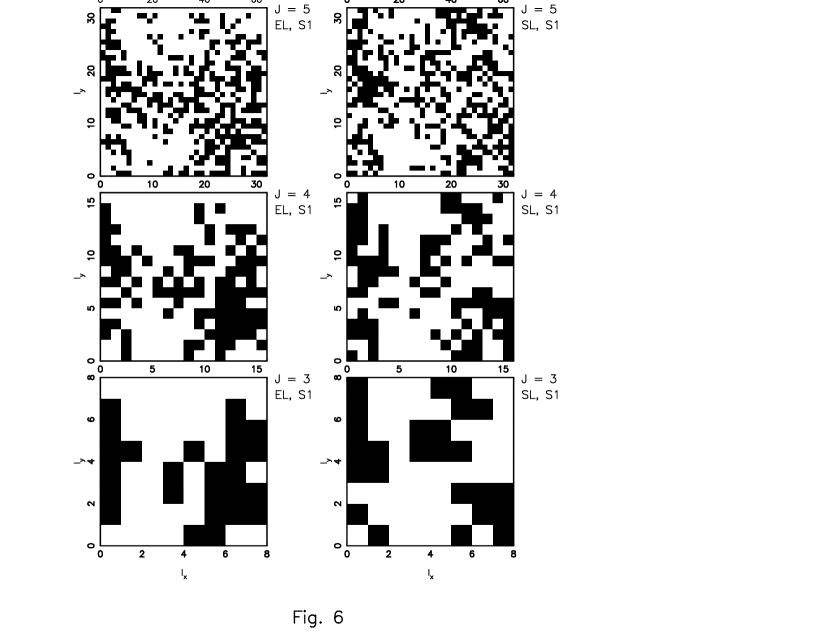
Figure 6: A simplified representation of Fig. 5. Dark area denote the overdense regions, $w_{j,l_{1};j,l_{2}}>\overline{w_{j}}$, and the blank area the underdense regions, $w_{j,l_{1};j,l_{2}}<\overline{w_{j}}$, where $j_{1}=j_{2}=j$.

A simplified representation of these fields is shown in Fig.6, in which the dark area represents the overdense regions, $w_{j,l_{1};j,l_{2}}>\overline{w_{{\bf j}}}$, and blank the underdense regions, $w_{j,l_{1};j,l_{2}}<\overline{w_{{\bf j}}}$. The ratio between the clustering strengths of the EL and SP on scale $j$ can be measured from Fig.6 by

$$a_{j}=\frac{({\rm dark\ area})_{EL}}{({\rm dark\ area})_{SP}}$$ (31)

Similar to the statistic $\tilde{b}^{(2)}_{j}$, to estimate the error of $a_{j}$, we generated 500 randomized samples of the ELs and SPs, and calculated the average $\overline{a_{j}}$ of these random samples. Fig. 7 plots the result of statistics $A_{j}$ defined as

$$A_{j}=\frac{a_{j}}{\overline{a_{j}}}.$$ (32)

The one $\sigma$ lines of both randomized and bootstrap re-sampling are also shown in Fig.7. The two error estimates gave about the same confidence level. The $j$-spectrum of $A_{j}$ is found to be significantly non-flat.

4.4 Statistics $B_{j}$

Since $A_{j}$ is based on statistic $w_{{\bf j},{\bf l}}$, one can expected that the statistic of $b^{(1)}_{j}$ of Eq.(21) will give the same conclusion. The 2-D extension of Eq.(21) is

$$b^{(1)}_{j_{1},j_{2}}=\frac{[\sum_{l_{1}=0}^{2^{j_{1}}-1}\sum_{l_{2}=0}^{2^{j_{2}}-1}|w_{{\bf j},{\bf l}}-\overline{w_{{\bf j}}}|]_{I}}{[\sum_{l_{1}=0}^{2^{j_{1}}-1}\sum_{l_{2}=0}^{2^{j_{2}}-1}|w_{{\bf j},{\bf l}}-\overline{w_{{\bf j}}}|]_{II}},$$ (33)

where we use absolute value $|w_{{\bf j},{\bf l}}-\overline{w_{{\bf j}}}|$ because for odd $n$, $\langle(w_{{\bf j},{\bf l}}-\overline{w_{{\bf j}}})^{n}\rangle$ has larger relative errors. We calculated $B_{j}^{(1)}$ defined as

$$B^{(1)}_{j}=\frac{\ b^{(1)}_{j,j}\ }{\overline{b^{(1)}_{j,j}}},$$ (34)

where $\overline{b^{(1)}_{j,j}}$ is the average of $b^{(1)}_{j,j}$ over 500 randomized samples of the ELs and SPs. The results of $B^{(1)}_{j}$ for the three fields are given in Fig. 8. The three fields S1, S2 and S3 show the same feature of the $j$ dependence. The mean SFCs and their variance from the randomized samples are also plotted in Fig.8. Like the statistics $A_{j}$, the spectrum of $B^{(1)}_{j}$ is non-flat with significance larger than 2 $\sigma$.

Since 2-D sample of galaxies is a $z$ (redshift) projection of their 3-D distribution. To study the influence of sample depth on our statistics, we calculated $B^{(1)}_{j}$ for samples of ELs and SPs with different limit magnitude $m$. Fig.9 plots the result of $B^{(1+)}_{j}$ which is the same as $B^{(1)}_{j}$ but for sample with limit magnitude $m=16.20$. In the case, the numbers of EL and SP galaxies are about 20-25% less than that of $m=16.44$. The $j$-spectra in Fig.9 have completely the same features as Fig.8. Therefore, conclusions drawn from Fig. 8 are insensitive to the depth of the samples.

In Figs.8 and 9, the $j$-dependence of bias is prominent on scales larger than 1 h^-1 Mpc, i.e. larger than the mean distance of nearest neighbors of galaxies, and therefore, the effect of shot noise is negligible.

5 Discussions and conclusions

We showed that, instead of one parameter $b$, Eq.(1) introduces a series of parameters $b^{(n)}_{j}$ and $\tilde{b}^{(n)}_{j}$ to describe the bias scale-dependence. The statistics of $\tilde{b}^{(n)}_{j}$ with different $n$ are independent from each others. The DWT analysis provides a simple and effective tool of systematically detecting the scale-dependence of bias parameters on various orders. This method is effective to be employed for analyzing galaxy samples which show morphology- and/or luminosity-segregation.

With this method we detected the $j$-spectra of $\tilde{b}_{j}^{(n)}$ and $b_{j}^{(n)}$ for the distributions of EL and SP galaxies of the APM-BGC samples. The general results indicate that for second order statistics, i.e. two-point correlation function and power spectrum, the bias is approximately scale-independent, but not so for higher order or phase-sensitive (non-Gaussian) statistics. The result is consistent with the following fact: most evidences for weak scale dependence of bias are from statistics of the two-point correlation functions and power spectrum (Kauffmann, Nusser & Steinmetz 1997), while the evidence for scale-dependence is from phase-sensitive statistics (Sigad et al. 1998). Therefore, the scale-dependence of galaxy bias may have the same origin as the non-Gaussianity of galaxy distribution. Linear evolution cannot cause non-Gaussianity of mass distributions if the initial perturbations are Gaussian. The scale-dependence of bias of galaxy distribution is most unlikely due to the non-linear evolution of gravitational clustering, and the non-local relationship between galaxy formation and their environment.

With this in mind, the information of bias scale-dependence is worth for developing models of galaxy formation. Indeed, despite the current detection of bias scale dependence is still very preliminary, the result is already able to set useful constraint on models of hierarchical clustering. In these models, galaxy correlations are generally assumed to be described by the hierarchical relation $\xi_{n}=Q_{n}\xi_{2}^{n-1}$ where $\xi_{n}$ is the $n$-th order correlation function, and $Q_{n}$ are constants (White 1979). If these hierarchical relations hold exactly, the second order (two-point) correlation function plus all constants $Q_{n}$ (which may be different for different types of galaxies) completely characterize the clustering of galaxies, including their higher order correlations. This is, all $\tilde{B}^{(n)}_{j}$ and $B^{(n)}_{j}$ can be represented by second order correlation function plus all (scale-independent) constants $Q_{n}$. Hence, if bias is scale-independent on second order, it will be scale-independent on all orders. Therefore, the non-flatness of $j$-spectra of $\tilde{B}^{(n)}_{j}$ and $B^{(n)}_{j}$ for sample APM-BGC implies that the hierarchical relations may not hold exactly, or the coefficients, $Q_{n}$, are scale-dependent. Similar conclusion has also been drawn from the detection of the scale-scale correlations of the Ly$\alpha$ forests of QSO absorption spectrum (Pando et al. 1998.) Thus, the detection of $\tilde{B}^{(n)}_{j}$ and $B^{(n)}_{j}$, joining with other higher order statistics, is effective to reveal the details of the hierarchical clustering scenario.

We thank Drs. J. Pando and Y.P. Jing for many helpful comments. ZGD and XXY were supported by the National Science Foundation of China.

Figure 1: The equal project of the APM bright galaxy distribution and three regions S1, S2 and S3, in which the wavelet analysis has been done. The top and bottom panels are for EL and SP galaxies respectively.

Figure 2: Two point angular correlation functions of EL (solid lines) and SP (dashed lines) galaxies in APM bright galaxy catalogue.

Figure 3: $\tilde{B}_{j}^{(2)}$ vs. j for three fields S1, S2 and S3. The mean of $\tilde{B}_{j}^{(2)}$ and 1 $\sigma$ error given by randomized samples are plotted by dot-dashed and dashed lines, respectively.

Figure 4: $\tilde{B}_{j}^{(3)}$ vs. j for three fields S1, S2 and S3. The mean of $\tilde{B}_{j}^{(3)}$ and 1 $\sigma$ error given by randomized samples are plotted by dot-dashed and dashed lines, respectively.

Figure 5: Reconstructed distributions of S1 on scales $j_{1}=j_{2}=6,5,4,3$ from top to bottom. Left side results are for EL galaxies and right for SPs. The bold contours are for $w_{j,l_{1};j,l_{2}}-\overline{w_{{\bf j}}}>2,3,4...\sigma_{j}$ from outside to inside successivefully, and the light contours denote the area with $w_{j,i_{1};j,l_{2}}/\overline{w_{{\bf j}}}\leq$ 1/2,1/8,1/32,1/128 from outside to inside successivefully.

Figure 7: $A_{j}$ vs. j for three fields (solid lines). It shows the mean of $A_{j}$ (thick solid lines), and 1 $\sigma$ errors given by randomized samples (dotted lines) and bootstrap-resampling (thin solided lines.)

Figure 8: $B_{j}^{(1)}$ vs. j for three fields (solid lines.) The mean of $B_{j}^{(1)}$ and 1 $\sigma$ error given by randomized samples are plotted by dot-dashed and dashed lines, respectively.

Figure 9: B${}^{(1+)}_{j}$ vs. j for three fields (solid lines.) The mean of B${}^{(1+)}_{j}$ and 1 $\sigma_{j}$ error given by randomized samples are plotted by dot-dashed and dashed lines, respectively.

References

- (1) Adler, R.J. 1981, the Geometry of Random Fields, Wiley, New York.
- (2) Bower, R.G., Coles, P., Frenk, C.S. and White, S.D.M. 1993, ApJ, 405, 403
- (3) Catelan, P., Coles, P., Matarreses, S. and Moscardini, L. 1994, MNRAS, 268, 966
- (4) Coles, P. 1993, MNRAS, 262, 1065.
- (5) Couchman, H.M.P. and Carlberg, R.G. 1992, ApJ, 389, 453
- (6) Daubechies, I. 1992, Ten Lectures on Wavelets, SIAM, Philadelphia
- (7) Davis, M. and Geller, M.J.. 1976, ApJ, 208, 13.
- (8) Deng, Z.G., Xia, X.Y., Fang, L.Z. and Börner, G. 1997, Astrophysical Report, No.2, 82
- (9) Dekel, A., Burstein, D. and White, S.D.M. 1996, astro-ph/9611108
- (10) Dekel, A. and Rees, M. 1987, Nature, 326, 455
- (11) Dressler, A. 1980, ApJ, 236, 351
- (12) Fang, L.Z. and Pando, J., 1997, in 5th Current Topics of Astrofundamental Physics, eds. N. Sanchez and A. Zichchi, World Scientific, Singapore, 616
- (13) Greiner, M., Lipa, P. & Carruthers, P. 1995, Phys. Rev. E, 51, 1948
- (14) Kaiser, N. 1984, ApJ, 284, L9
- (15) Kauffmann, G., Nusser, A. and Steinmetz, M. 1997, MNRAS, 286, 795
- (16) Loveday, L, Peterson, B. A., Efstathiou, G, and Maddox S. J., 1992, ApJ, 390, 338
- (17) Loveday, L, 1996, MNRAS, 278, 1025
- (18) Loveday, L., Maddox, S.J., Efstathiou, G. & Peterson, B.A. 1995, ApJ, 442, 457
- (19) Meyer, Y. 1993, Wavelets: Algorithms and Applications, SIAM, Philadelphia
- (20) Mo, H.J., Jing, Y.P. & Börner, G. 1992, ApJ, 392, 452
- (21) Mo, H.J., Jing, Y.P. and White, S.D.M. 1996, MNRAS, 284, 189
- (22) Pando, J. and Fang, L.Z., 1996, ApJ, 459, 1
- (23) Pando, J. and Fang, L.Z., 1998, Phys. Rev. E57, 3593
- (24) Pando, J., Lipa, P., Greiner, M. and Fang, L.Z., 1998, ApJ, 469, 9
- (25) Peebles, P. J. E., 1980, The Large Scale Structure of the Universe, Princeton, NJ., Princeton Univ. Press.
- (26) Rees, M. 1985, MNRAS, 213, 75p
- (27) Saunders, W., Roiwan-Robinson, M., & Lawrence, A. 1992, MNRAS, 258, 134
- (28) Sigad, Elder, A., Dekel, A., Strauss, M.A. & Yahil, A. 1998 ApJ, 495, 516
- (29) Staruss, M.A., Davis, M., Yahil, A. and Huchra, J.P. 1992, ApJ, 385, 421
- (30) Vanmarcke, E. 1983, Random Field, MIT Press.
- (31) Xia, X.Y., Deng, Z.G and Zhou, Y.Y. 1987, in Observational Cosmology, eds. Hewitt, A., Burbidge and L.Z.Fang, Reidel Pub. Co. 363
- (32) Yamada, M. and Ohkitani, K. 1991, Prog. Theor. Phys., 86, 799
- (33) White, S.D.M. 1979, MNRAS, 186, 145