Explosive Nucleosynthesis: Coupling Reaction Networks to AMR Hydrodynamics

K. Kifonidis¹, T.  Plewa^2,1, E.  Müller<sup>1

1</sup> Max-Planck-Institut für Astrophysik, Karl-Schwarzschild-Strasse 1, D-85740 Garching, Germany
² Nicolaus Copernicus Astronomical Center, Bartycka 18, 00716 Warsaw, Poland

1.1 Introduction

Observations of SN 1987A revealed that extensive mixing had taken place in the exploding envelope of the progenitor Sk -69 202. Especially the early detection of X and $\gamma$-rays [7], [15], the broad profiles of infrared Fe II and Co II lines [6], [9] as well as modelling of the light curve [1], [22] indicated that $\rm{}^{56}Ni$ was mixed from the layers close to the collapsed core, where it was explosively synthesized, out to the hydrogen envelope where the highest expansion velocities occurred.

Multidimensional hydrodynamic models of the late phases of the explosion (starting several minutes after core bounce) while successful in confirming that mixing due to Rayleigh-Taylor instabilities did indeed occur after the explosion shock had passed the C,O/He and He/H interfaces, have hitherto failed to yield the amount of mixing observed [8], [10], [17]. However, Herant and Benz [11] have shown that velocities in line with the observations could be obtained if one artificially mixed $\rm{}^{56}Ni$ in the very early phases of the explosion out to layers which later suffer from the Rayleigh-Taylor instabilities.

In the light of results from recent multidimensional simulations of the (neutrino driven) explosion mechanism itself which revealed large scale anisotropies, mixing and overturn due to convective motions taking place within about one second after core bounce behind the revived supernova shock, it has been argued [12], [14] that a physically satisfactory mechanism has been found which might lead to the required amount of “premixing” and thus resolve the nickel problem. However, only very preliminary multidimensional computations exist to date which attempt to follow the mixing of nickel from the moment of nucleosynthesis until it appears in the hydrogen envelope of the exploding star [18]. Despite constant growth in computer resources and steady advances in numerical algorithms such simulations still pose a formidable task due to the large range of spatial and temporal scales which have to be resolved. Therefore, most of the computations hitherto performed started from artificial spherical models of the explosion itself.

In recent years the technique of Adaptive Mesh Refinement (AMR) has been applied to several astrophysical problems (cf. [5], [19]) and should allow a consistent modelling of the complete evolution in two dimensions. In this contribution we address some of the computational difficulties encountered when trying to apply AMR to explosive nucleosynthesis and supernova envelope ejection.

1.2 Adaptive Mesh Refinement

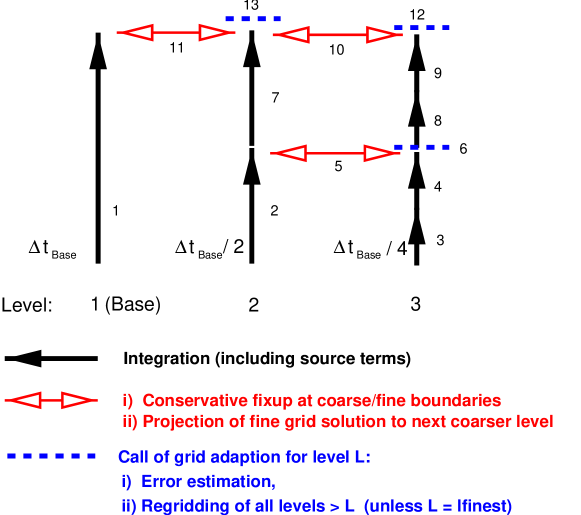
Figure 1: Integration of the grid hierarchy over a single base level time step for 3 levels of refinement with a constant refinement factor $r=2$. Note that grids at level $l+1$ have to be evolved with time steps $\Delta t_{l}/r$. The numbers indicate the actual sequence of operations to be carried out. A regridding frequency of $K=2$ was chosen in this example.

AMR is an algorithm for the efficient solution of systems of time-dependent, hyperbolic partial differential equations [2]. An extended version of the basic AMR algorithm applied to the Euler equations of ideal, compressible flows has been discussed in [3]. In essence, AMR provides a way to automatically adjust the computational grid resulting from the discretization of the differential equations subject to the estimated error of the solution. Since in many cases this error is large only in some regions of the computational domain AMR usually offers large savings in CPU time and memory usage.

The AMR algorithm constructs and continuously updates a tree of nested grid meshes or patches located on different levels in the tree hierarchy. Each level can be formed out of one or more patches with the resolution changing between levels from lower (coarse) to higher (fine) levels by arbitrary (but integer) factors in each dimension. Patches forming a single level may partially overlap each other or may cover distinct regions of the computational domain, but those belonging to different levels must necessarily be “properly nested”, i.e.  patches on a given level must be totally covered by one or more patches located on the next coarser level.

Integration of the grids proceeds starting from the base level grid of the lowest resolution, which covers the entire computational domain, and recursively continues through the higher levels of the grid hierarchy (Fig. 1). Some amount of communication between the different levels is needed in order to obtain a consistent solution. This includes averaging of the solution obtained on fine patches and its projection down to parent patches. Furthermore, special attention is required at boundaries separating coarse and fine grid cells. The integration of fine grids is carried out using boundary (ghost) zones which might have to be initialized by interpolating data from coarser levels. In the general case, numerical fluxes calculated with higher resolution will differ from fluxes calculated with lower resolution. To ensure global conservation a correction pass over all coarser grid cells abutting fine grid cells is needed once both grid levels have been integrated to the same time. We refer the reader to [3] for a more detailed description of this procedure.

Finally, every $K$ time steps on a given level an error estimation procedure is invoked, which yields an estimate of the local truncation error. The regions where this value exceeds some predefined threshold, $\epsilon$, are marked and later covered with new grid patches of higher resolution. Thereby flow features requiring high resolution like shocks, contact discontinuities or strong gradients in the solution are always followed with the higher level grids while regions where the flow is essentially smooth are calculated at lower resolution. It is important to note in this context that newly created fine grids might have to be initialized with data obtained by interpolation from underlying coarser grids. As we will show below this procedure may lead to serious numerical problems especially for multi-component flows.

1.3 Numerical tests

In our numerical investigations we considered the problem of a supernova explosion for a 15 $\rm M_{\odot}$ model progenitor of Woosley, Pinto and Ensman [23] in one dimension assuming spherical symmetry and using the amra code [20]. The hydrodynamic equations were solved with the direct Eulerian version of the Piecewise Parabolic Method (PPM) as implemented in the prometheus code [8] although amra can be used in conjunction with any hydrodynamic scheme.

After removing the model’s iron core the explosion was initiated by depositing an energy of $10^{51}$ ergs in form of a thermal bomb into the innermost region of the silicon shell. We used five levels of refinement, with 256 zones on the base grid (level 1) and refinement factors of 2, 4, 6, and 8 for patches on levels 2, 3, 4, 5 respectively. This gave us an effective resolution of 98 304 equidistant zones. The computational domain extended from $1.4\times 10^{8}$ cm up to $3.8\times 10^{11}$ cm and covered about the inner 1/10 th of the star. Besides $\rm{}^{1}H$, the 13 $\alpha$-nuclei from $\rm{}^{4}He$ to $\rm{}^{56}Ni$ were included. A realistic equation of state was used that contained contributions from all considered nuclei as well as electrons, photons and $e^{+}$/$e^{-}$-pairs. Gravity was taken into account and included the contribution from the collapsed central core as well as self-gravity of the envelope. The code was optimized to run efficiently on CRAY shared memory systems.

The solution of the coupled system of hydrodynamic and nuclear rate equations neccessitates a detailed description of the chemical composition within the hydrodynamic scheme. In prometheus this is achieved by solving additional continuity equations for each fluid component, with the partial densities, $\rho X_{i}$, (where $X_{i}$ denotes the mass fraction of species $i$) as state variables. This extension of basic PPM is reflected within amra in two ways. Firstly, the fixup procedure for fluxes at fine-coarse boundaries is done for the partial densities in a similar way as for the other conserved quantities. Secondly, fractional masses are interpolated conservatively when boundary data for fine patches are needed or when the hydrodynamic state for the interior of a newly created fine patch has to be provided. Both steps may lead to serious numerical problems due to the fact that the interpolation scheme does not guarantee that the total gas density will remain equal to the sum of partial densities after interpolation. One might expect that the magnitude of this problem will be large whenever the new patch is created in regions where the partial densities vary significantly. Furthermore, the degree of mismatch between the total and partial densities should decrease with increasing degree of smoothness. The latter can efficiently be controlled using the threshold for truncation error. In what follows we ignore for the moment nuclear reactions and focus on this interpolation problem by presenting results obtained for the same initial data but varying truncation error thresholds.

Figure 2

Figure 2: Left: Mass fraction profiles for our test problem after 34.9 s of evolution. By this time the shock has reached a radius slightly larger than $3\times 10^{10}$ cm and is tracked with a single level 5 patch. The error estimation algorithm was applied only to $(\rho,\rho u,\rho E_{\rm tot})$ and a local truncation error of $\epsilon=0.1$ was used. Large errors in mass fractions can clearly be seen in the central region of the grid. Right: Same as left panel but with $\epsilon=0.01$. In spite of the increased accuracy (by a factor of ten) the solution is still flawed.

displays the chemical profiles obtained when the truncation error is estimated only for the conserved quantities ($\rho$, $\rho u$, $\rho E_{\rm tot}$) with $\epsilon=0.1$ and $\epsilon=0.01$ in the left and right panel, respectively. In both cases large errors in the distribution of species are visible. Using a smaller $\epsilon$ helps in resolving the outer edge of the silicon shell ($r\approx 1-2\times 10^{10}$ cm), but some low-amplitude noise can still be seen at $r\approx 1.5\times 10^{10}$ cm. However, the computed distribution of $\rm{}^{28}Si$ in the core does not seem to be sensitive to this mild improvement in overall accuracy and in addition to low-amplitude noise a conspicuous undershoot is present at $r\approx 10^{9}$ cm for the $\epsilon=0.01$ case. The quality of the solution improves when in addition to the error estimation for $(\rho,\rho u,\rho E_{\rm tot})$ we also estimate the truncation error for the partial densities (Fig. 3).

Figure 3: Left: Same as Fig. 2 but with $\epsilon=0.1$ for $(\rho,\rho u,\rho E_{\rm tot})$ and additional flagging of the partial densities, $\rho X_{i}$, with $\epsilon_{X}=0.1$. Right: Same as left panel but with $\epsilon=0.01$ and $\epsilon_{X}=0.01$.

With $\epsilon=0.1$ and $\epsilon_{X}=0.1$ most of the material interfaces located just below the helium shell are resolved and no large errors in the silicon distribution are present. With increased accuracy ($\epsilon=0.01$, $\epsilon_{X}=0.01$) the finest level patches extend from the centre of the grid further out and help in keeping the chemical composition smooth. The outer edge of the silicon core is now covered with level 4 patches and all chemical discontinuities are modelled using the highest resolution. However, the errors are not totally eliminated. The silicon abundance is still affected near $r\approx 7\times 10^{8}$ cm. From our numerical experiments we found that using $\epsilon=0.001$ and $\epsilon_{X}=0.01$ finally eliminates the problem (cf. the left panel of Fig. 4) with patches on the finest level now extending from the inner boundary to radii slightly above $r\approx 10^{9}$ cm.

Figure 4: Left: Same as Fig. 2 but with $\epsilon=10^{-3}$ and $\epsilon_{X}=10^{-2}$. All errors have disappeared. Note the changes in the distribution of grid patches. The larger number of level 4 and level 5 patches resulted in an increase in CPU-time of about a factor of 5 and 3.6 as compared to the first and second case shown in Fig. 2, respectively. Right: Chemical composition at $t=0.5$ s for our run including nuclear burning (see text). At this time nearly all nuclear reactions have frozen out. Nucleosynthesis has taken place mainly in the former silicon shell. Following the inner layers, where peak temperatures were sufficiently high to synthesize $\rm{}^{56}Ni$, incomplete Si-burning has led to a zone dominated by $\rm{}^{32}S$, $\rm{}^{36}Ar$, and $\rm{}^{40}Ca$. The C/O-core of the star is almost completely covered with the finest resolution ($\Delta r\approx 39$ km). Abrupt changes in composition in this region are a consequence of coarse zoning in the initial model. Note that, in contrast to the other runs, the entire grid extends up to $1.2\times 10^{6}$ km in this case.

In the right panel of Fig. 4 we finally present results obtained with an $\alpha$-chain network of 27 reactions for our 13 $\alpha$-nuclei. The network was coupled to the hydrodynamics as described in [16]. The same explosion energy as for the other runs was also adopted for this setup. However, the computational domain extended from $r=1.4\times 10^{8}$ cm to $r=1.2\times 10^{11}$ cm. Five levels of refinement, 120 zones on the base grid and refinement factors of 2, 4, 4 and 8 were used. The truncation error thresholds were set to $\epsilon=0.001$ and $\epsilon_{X}=0.01$. In addition flagging of density contrasts above 0.1 was employed. The obtained solution does not differ from a corresponding single grid model computed using 30 720 equidistant zones and demonstrates that with a cautious use of the AMR technique it is possible to obtain physically correct results. Moreover, the speedup achieved in calculating the first $6.4\times 10^{-2}$ s of evolution as compared to the single grid run amounted to a factor of 8.4 on a single node of an IBM SP2. We note here that there is some overhead associated with AMR because the source terms have to be computed also in the error estimation procedures. This is especially important during this early phase, when the solution of the nuclear network dominates the computational time. But since cooling due to the strong expansion leads to a rapid freezeout of nuclear reactions, we may expect AMR to offer even larger savings in CPU time during the late evolutionary phases. We were not able to continue this comparison further in time, however, as the computational cost for the single grid run turned out to be prohibitively high.

In the future, we plan to use amra to study the problem of nucleosynthesis and mixing in two dimensions starting shortly after shock stagnation, when shock revival due to neutrino heating and convective motion begins, through the stage where the aspherical shock overruns the Si and O shells leading to an aspherical distribution of newly synthesized nuclei, up to the development of the Rayleigh-Taylor instability. Current multidimensional simulations of the delayed explosion mechanism (cf. [13], [4], [14]) indicate that explosive burning will partly proceed for electron fractions well below $Y_{e}\approx 0.5$ and thus results in neutron rich isotopes. In order to avoid a contamination of the interstellar medium with the wrong nucleosynthetic products, fallback of this material onto the central remnant in the late stages of the explosion was suggested. Therefore, another goal of such computations is to determine the actual location of the mass cut and to provide the link needed to test the current ideas behind the delayed explosion mechanism by confronting the ejected nucleosynthesis products with observations.

Acknowledgements

We are very grateful to Stanford Woosley for providing us with various progenitor models which we have used to construct our initial data. The work of TP was partly supported by the grant KBN 2.P03D.004.13 from the Polish Committee for Scientific Research. The simulations were performed on the IBM SP2-P2SC and CRAY J916/16512 located at the Rechenzentrum Garching.

References

- [1] W.D. Arnett, J.N. Bahcall, R.P. Kirshner, S.E. Woosley, Ann. Rev. Astron. Astrophys. 27 (1989) 341.
- [2] M. Berger and J. Oliger, J. Comp. Phys. 53 (1984) 484.
- [3] M. Berger and P. Colella, J. Comp. Phys. 82 (1989) 64.
- [4] A. Burrows, J. Hayes, B.A. Fryxell, ApJ 450 (1995) 830.
- [5] R. Cid-Fernandes, T. Plewa, M. Różyczka, J. Franco, R. Terlevich, G. Tenorio-Tagle, W. Miller, MNRAS 283 (1996) 419.
- [6] S.W.J. Colgan, M.R. Haas, E.F. Erickson, S.D. Lord, D.J. Hollenbach, ApJ 427 (1994) 874.
- [7] T. Dotani et al., Nature 330 (1987) 230.
- [8] B.A. Fryxell, E. Müller, W.D. Arnett, ApJ 367 (1991) 619.
- [9] M.R. Haas, S.W.J. Colgan, E.F. Erickson, S.D. Lord, M.G. Burton, D.J. Hollenbach, ApJ 360 (1990) 257.
- [10] M. Herant and W. Benz, ApJ 370 (1991) L81.
- [11] M. Herant and W. Benz, ApJ 387 (1992) 294.
- [12] M. Herant, W. Benz, S. Colgate, ApJ 395 (1992) 642.
- [13] M. Herant, W. Benz, W.R. Hix, C.L. Fryer, S. Colgate, ApJ 435 (1994) 339.
- [14] H.-Th. Janka and E. Müller, A&A 306 (1996) 167.
- [15] S.M. Matz, G.H. Share, M.D. Leising, E.L. Chupp, W.T. Vestrand, W.R. Purcell, M.S. Strickman, C. Reppin, Nature 331 (1988) 416.
- [16] E. Müller, A&A 162 (1986) 103.
- [17] E. Müller, B.A. Fryxell, W.D. Arnett, A&A 251 (1991) 505.
- [18] S. Nagataki, T.M. Shimizu, K. Sato, ApJ 495 (1998) 413.
- [19] H. Nussbaumer and R. Walder, A&A 278 (1993) 209.
- [20] T. Plewa and E. Müller, in preparation.
- [21] F.-K. Thielemann, K. Nomoto, M. Hashimoto, ApJ 460 (1996) 408.
- [22] S.E. Woosley, ApJ 330 (1988) 218.
- [23] S.E. Woosley, P.A. Pinto, L. Ensman, ApJ 324 (1988) 466.