Dust Extinction and Molecular Cloud Structure: L977

Abstract

We report results of a near–infrared imaging survey of L977, a dark cloud in Cygnus seen in projection against the plane of the Milky Way. We use measurements of the near–infrared color excess and positions of the 1628 brightest stars in our survey to measure directly dust extinction through the cloud following the method described by Lada et al. (1994). We spatially convolve the individual extinction measurements with a square filter 90^′′ in size to construct a large–scale map of extinction in the cloud. We integrate over this map to derive a total mass of $M_{L977}=(660\pm 30)\ (D/500pc)^{2}$ M_⊙ and, via a comparison of source counts with predictions of a galactic model, estimate a distance to L977 of 500 $\pm$ 100 pc. We find a correlation between the measured dispersion in our extinction determinations and the extinction which is very similar to that found for the dark cloud IC 5146 in a previous study. We interpret this as evidence for the presence of structure on scales smaller than the 90^′′ resolution of our extinction map.

To further investigate the structure of the cloud we construct the frequency distribution of the 1628 individual extinction measurements in the L977 cloud. The shape of the distribution is similar to that of the IC 5146 cloud. Monte Carlo modeling of this distribution suggests that between 2 $<$ A_V $<$ 40 mag (or roughly 1 $<$ $r$ $<$ 0.1 pc) the material inside L977 is characterized by a density profile $\rho\,(r)\propto r^{-2}$. Direct measurement of the radial profile of a portion of the cloud confirms this result.

At the lower galactic latitude of L977, we find both the mean and dispersion of the infrared colors of field stars to be larger than observed toward IC 5146. This produces an increase of about a factor of 2 in the minimum or threshold value of extinction that can be reliably measured toward L977 with this technique. Nevertheless the accuracy in an extinction map pixel is not significantly different toward L977 due to the increased number of field stars at this latitude. We also find an increase in the number of detected giant stars at the lower galactic latitude of the survey by almost a factor of two. Most of these excess stars suffer extraneous extinction and are probably red giants seen along the disc of the Milky Way up to distances $\sim$ 15 kpc and reddened by unrelated background molecular clouds along this direction of the Galaxy. We discuss a possible application of this observable to galactic structure studies on the plane of the Galaxy.

1 Introduction

Knowledge of the distribution of mass within molecular clouds is critical for the understanding of how molecular clouds form, evolve, and ultimately produce stars and planets. Dust is the most reliable tracer of the undetectable molecular hydrogen gas, which is the primary component of the mass of molecular clouds. The most straightforward way to measure the dust content of a molecular cloud is through direct measurements of dust extinction of background starlight. This can be optimally done at near infrared wavelengths where the dust opacity is modest and the reddening law appears universal (Jones & Hyland 1980; Cardelli et al. 1989; Martin & Whittet 1990; Whittet et al. 1993). The determination of gas mass from dust extinction is relatively straightforward and relies on basically one observationally well established assumption: a constant gas–to–dust ratio (Lilley 1955; Jenkins & Savage 1974; Bohlin et al. 1978).

Recently, Lada et al. (1994) demonstrated that large scale near-infrared imaging surveys of dark clouds can directly trace the distribution of dust extinction and column density through a molecular cloud at considerably higher angular resolution and greater optical depth than previously possible from pure star counts (Bok 1937). In fact, Lada et al. (1994) developed a method for measuring and mapping extinction which is more direct and fundamentally more powerful than star counts made at any wavelength. Their method uses: 1) measurements of infrared (H[1.6$\mu$m]$-$K[2.2$\mu$m]) color excess, 2) knowledge of the near–infrared extinction law, and 3) techniques of star counting to derive directly and map extinction through a cloud. Also, since the method is based on pencil beam measurements of the extinction, it can give information about both the large–scale and small–scale structure of a molecular cloud.

We have two main motivations for the present paper. First, we want to apply the Near–Infrared Color Excess method used by Lada et al. (1994) (hereafter, NICE method) to a different molecular cloud to compare its physical conditions with those derived for IC 5146. Second, because the information on the spatial distribution of dust derived from this method is a function of both the surface density and colors of stars detected through the target cloud, we want to test the applicability of the method against rich background star fields at low galactic latitudes.

L977 is part of dark globular filament GF7 in the Cygnus complex (Schneider & Elmegreen 1978) and lies against a rich background of field stars towards the warped plane of the Galaxy ($l=90$^∘, $b=2$^∘). There is no obvious sign of ongoing star formation in this cloud. Although three IRAS point sources lie in the direction of L977, their colors are indicative of infrared cirrus emission rather than pre–main sequence objects. This dark cloud is in the Dobashi et al. (1994) ¹³CO large scale survey of the Cygnus region as an isolated cloud and free from confusion with other molecular clouds. Apart from this survey L977 is virtually unstudied.

We describe the acquisition and reduction of the observations in Section 2, the results in Sec. 3, the analysis and discussion in Sec. 4, and we summarize our conclusions in Sec. 5 of the paper.

2 Observations and Data Reduction

We obtained near-infrared imaging observations of L977 using the National Optical Astronomy Observatory (NOAO) Simultaneous Quad Infrared Imaging Device (SQIID) on the Kitt Peak National Observatory (KPNO) 1.3m telescope in 1994 October. SQIID is equipped with four 256 $\times$ 256 platinum silicide (PtSi) focal plane arrays. Dichroic mirrors allow simultaneous observations at four infrared wavelength bands: $J$ (1.25 $\mu$m), $H$ (1.65 $\mu$m), $K$ (2.20 $\mu$m), and $L$ (3.4 $\mu$m). For this project, we obtained data only in the $J$, $H$, and $K$ bands. The optics provide a field of view of approximately 5^′.5 $\times$ 5^′.5 and a resolution of 1^′′.36 per pixel at $K-$band.

We observed a total of 17 fields at each wavelength band towards L977 covering 336 arcmin² on the sky in a roughly 4 $\times$ 4 mosaic grid. The area surveyed in the 3 NIR bands is represented in Figure 1 as the central square overlaid on the Digitized Sky Survey red POSS plate . The L977 molecular cloud is readily seen as the zone of obscuration against the rich star field that characterizes this region of the galaxy. The fields observed in the direction of our target cloud were spatially overlapped by $\sim$1^′.5 in both right ascension and declination, allowing for both the accurate positional placement of the mosaicked fields and redundancy of our photometric measurements of sources located in the overlapped regions.

To characterize the distribution of background/foreground field stars a total of 7 control fields were observed at each band. Since our two target clouds lie against a complicated background of field stars, very near the galactic plane, special care was used in choosing the control fields regions. These fields were chosen to be as close as possible to our target cloud, equally distributed around it, but free from any significant molecular cloud material contamination through inspection of the ¹³CO survey (Dobashi et al. 1994) and the Palomar Sky Survey Prints. The boxes to the East and to the West of L977 in Figure 1 show the regions where these control fields were taken. They are spatially separated by 1 degree in the sky ($\Delta l=0.7$^∘, and $\Delta b=0.8$^∘). The control field images were not overlapped. The integration time in each filter for observations both on and off L977 was 180 seconds. All fields were observed twice, with a 15^′′ offset between observations.

2.1 Reduction Procedure

We used a combination of the standard Image Reduction and Analysis Facility (IRAF) routines and custom software for data reduction. The data frames were reduced in the following 3 step procedure: a dark frame was subtracted from each data frame, the resulting dark–subtracted frame was then divided by a flat field, and finally the value of the local sky was subtracted from the dark subtracted flat fielded frame. The dark frames are averages of 20 individual dark images acquired at the beginning and end of each night. The flat fields used for each filter were constructed by median filtering the 20 time-neighboring (at roughly the same airmass) dark subtracted images and found to be indistinguishable within the errors. These flat-field images were then autonormalized before division into the appropriate dark subtracted data frames. The local sky was taken as the mean of the dark–subtracted flat–fielded data frame. A conventional sky removal procedure (direct frame–by–frame sky subtraction) was performed on 6 typical data frames for comparison with the adopted reduction procedure. The photometric results from both image reduction procedures were then compared and found to be identical within the photometric errors discussed below.

2.2 Source Extraction and Photometry

Sources were identified and counted using the DAOFIND routine (Stetson 1987) within the IRAF package. DAOFIND was run on each image separately, using a full width at half maximum (FWHM) of the point spread function between 1.7 to 2.0 pixels and a single pixel finding threshold equal to 5 times the mean noise of each image. The results and images were carefully inspected. The DAOFIND coordinate files were edited to remove bad pixels, non-stellar objects and artifacts misidentified as stars and to append stellar sources that were not originally extracted by the finding routine. Photometry was then obtained for all extracted stars in the final images using APPHOT with a variety of different apertures. Photometric measurements were independently obtained for each dithered pair of images toward each field. Custom stellar matching software was used to compare the magnitudes obtained for each dithered stellar pair. A series of tests were then performed on this photometric database. For the various apertures, plots of the difference magnitudes for each star versus the mean magnitude showed no systematic offset, while still displaying the expected flared errors at faint magnitudes. Further, plots of the difference magnitude versus the internal photometric uncertainties, returned by APPHOT, showed no unexpected effects or features. We conclude that the internal APPHOT uncertainties are reasonably good estimators of the true photometric uncertainties. In Figure 2 we plot the photometric errors, as returned by APPHOT, in the colors ($(J-H)$ open triangles; $(H-K)$ filled triangles) as a function of magnitude $(H)$ for stars observed toward L977.

For the photometry presented here, the 2.5 pixels (3^′′.4) aperture was chosen. This aperture size corresponds to $\sim$ 2–3 times the FWHM of the typical point spread function for our SQIID data. Sky values around each source were determined from the mode of pixel intensities in an annulus having an inner radius of 10 pixels and an outer radius of 20 pixels. The average number of stars found per frame was about 200 at K, reducing the need for PSF fitting photometric extractions. Using an aperture with a 2.5 pixel radius insured that the flux from $\sim$90% of the sources was not contaminated by the flux from nearby stars. However, this aperture was too small to contain all the flux from a source. Therefore, to account for the missing flux, multi-aperture photometry was performed for each image on all bright (m_J,H,K $<$ 12), isolated sources. For these sources, the flux obtained in the 2.5 pixel radius aperture was compared with flux measured in a larger 3, 4, 5, 7, and 9 pixels radius apertures and the fraction of the total source flux falling within the 2.5 pixel radius aperture was then determined. Typically, the 2.5 pixel radius aperture was found to contain approximately 90% of the total source flux. A similar result was reached by Barsony et al. (1997) for SQIID observations of the $\rho$ Ophiuchi cloud core. The instrumental magnitudes for all extracted SQIID sources were corrected to account for the missing flux.

We confirm the tendency for stars imaged onto the outer 10% of the PtSi SQIID arrays to show unusual colors (e.g., Lada et al. 1994). To remove this effect, stars imaged onto the outer 10% of the array had their corresponding photometry rejected. All surviving data were then merged into two databases: the target and the control database. Duplicate stars from neighboring target frames (up to four), were identified and their magnitudes averaged.

Photometric calibration for our data was accomplished using the list of Elias standard sources (Elias et al. 1982). Eight standards were observed on the same nights and through similar airmasses as were observations of on field and off field images and were used to independently establish the photometric zero points for each of the filters. Otherwise, we elected to use the SQIID camera filters and arrays as our photometric system and have applied no further adjustments (e.g., color-corrections) to our measurements since the SQIID photometric system seems close to the Elias et al. (1982) photometric system (CIT) (Kenyon, Lada, & Barsony 1998). The standards were observed at nearly the same airmasses as the L977 fields and since atmospheric infrared extinctions are very small ($\;\buildrel<\over{\sim}\;$0.1 magnitudes per airmass), our reported magnitudes and colors are likely not in error by much more than their photometric uncertainties determined by APPHOT.

2.3 Completeness Limits

In order to estimate the completeness limits of our observations, we compared the number of stars identified, as a function of magnitude, on pairs of dithered images in each band. DAOFIND and PHOT were run on the overlapping regions of 5 pairs of dithered off field images, using the same criteria described in 2.3. The apparent magnitude distribution of stars that were identified and matched across the dithered pairs of images was compared to the magnitude distribution of stars that were found in only one of the image pairs. From this comparison, we estimate that the identification of sources in the individual image frames is $\sim$ 90% complete to m_J = 15.5, m_H = 14.5 and m_K = 13.5. These completeness limits are extended another 0.4 magnitudes after combining the paired images obtained in each on and off position. For the $K-$band observations we also estimated the survey completeness to fainter magnitudes and found it to be roughly 85% between 13.5–14 mag, 75% between 14–14.5 magnitudes and only 60% between 14.5–15.0 magnitudes for the individual dithered images.

2.4 Positions

We determined absolute $\alpha$ and $\delta$ positions for each individual source identified by our near-infrared observations of L977. We used a centering algorithm in APPHOT to obtain center positions for the sources in pixels. Duplicate stars on adjacent frames were used to register the relative pixel positions of the individual SQIID frames onto a single positional grid. Pixel positions were converted to equatorial coordinates using observations of 3 stars from Hubble Space Telescope Guide Stars Catalog (GSC) that were detected within our grid. Both the plate scale (1.358 arcsec pixel^-1 at $K-$band) and grid orientation relative to north (+0.71^∘) were derived from matching the positions of these stars with their pixel coordinates. The resulting coordinate transformation was applied to all stars in the image to obtain their positions in the GSC astrometric system. We re–measured the position of the GSC stars and determined an average difference to the absolute positions of 0.5^′′. The measured standard deviation of the differences between the derived and absolute coordinates of the reference stars was found to be 0.2^′′.

3 Results

3.1 Color–Color Diagrams

The results of the NIR photometry for the control regions (defined in Figure 1 by the boxes to the East and to the West of L977) are presented in Figure 3. These plots display only those stars in each region for which photometric uncertainties in each band were less than 0.10 magnitudes. Also plotted as a solid line on both color–color diagrams is the locus of points corresponding to unreddened main sequence and giant stars (Koornneef 1983). The two parallel dashed lines define the reddening band for both main sequence and giant stars using the reddening law of Rieke & Lebofsky (1985). The typical photometric error for both colors for a $K=14$ star — roughly a 10 sigma detection — is displayed in the upper corner of both diagrams. There are a total of 303 sources detected in the East control field region and 219 in the West control field region. The surface density of detected sources in the $JHK-$bands for the East control field region ($\Sigma_{E}$) is slightly higher than in the West control field region ($\Sigma_{W}$) — $2.6$ vs. $2.5$ stars ($\sigma<0.1$) per square arcmin — most likely due to the fact that the East control field region is almost 1^∘ closer to the Galactic plane. The mean $(H-K)$ and $(J-H)$ colors and dispersions for the two regions are nevertheless the same to 2 significant figures:

$$<(H-K)>_{E}\>\,=\>\,<(H-K)>_{W}\>\,=0.20\pm 0.13\>\,$$

$$<(J-H)>_{E}\>\,=\>\,<(J-H)>_{W}\>\,=0.56\pm 0.27\>\,$$

The spatial distribution of sources in the color–color plane is apparently very similar for both control regions. We used a 2D version of the Kolmogorov–Smirnov test (Peacock 1983; Fasano & Franceschini 1987; Press et al. 1992) to compare both East and West control fields color distributions and we found a high probability (0.74) that the sources in both control fields were randomly drawn from the same population. Sources in both the East and West control fields are distributed in two distinct groups: 1) a blue group that is roughly uniformly distributed around the point ($(H-K)$, $(J-H)$) $=$ (0.07, 0.35) corresponding to the color of an mid G main sequence star (Koornneef 1983), and 2) a red group which has an elongated distribution along the direction of the reddening vector and has colors ($(H-K)$, $(J-H)$) $=$ (0.20 to 0.40, 0.60 to 1.10) corresponding to the colors of either late type giants or reddened early K giants/main sequence stars.

In Figure 4 we show the $JHK$ color–color diagram for the L977 field defined in Figure 1 by the central square region. The main sequence and giant locus, as well as the photometric errors are the same as in Figure 3. The displacement in this diagram caused by 5 visual magnitudes of extinction is represented by the solid line to the left of the reddening vector. There are 809 sources simultaneously detected in the $JHK-$bands with photometric errors below 0.10 magnitudes at each band. The large majority of sources is distributed along the reddening vector. Of the 809 high–quality photometry sources shown, 84 sources are located below the reddening band and 79 sources are located above it. Hence, the number of infrared excess sources detected toward the L977 field is negligible. The ten most deviant sources from the reddening band are all faint and have magnitudes very close to the 10 sigma detection limit. The average K magnitude of this sub-sample of 10 stars is $<K>$ $=$ 13.60 $\pm$ 0.26 magnitudes. Comparison of Figures 3 and 4 strongly suggests that the vast majority of stars observed toward the L977 molecular cloud are field stars unrelated to the cloud. Moreover, a significant number of these sources are clearly reddened background objects observed through the cloud. Because the surveyed area (Figure 1) included a substantial region in the sky suffering negligible extinction from L977 we are able to retrieve the results obtained in the control field regions, namely the blue and red grouping of sources with the same characteristics and locations on the color–color plane.

3.2 Determination of the NIR Extinction Law

Although we have assumed the extinction law of Rieke & Lebofsky (1985) for comparison with our data, we can use our observations to derive the NIR extinction law, $E(J-H)/E(H-K)$, in this cloud. This can be done from comparison between the color of stars seen through L977 and color of stars in the control fields. We have to assume that the background population to L977 is well characterized by the stars in the control fields. As we shall see in section 4.1, that is a valid assumption. However, the dispersion in the color of stars in the control fields at these low galactic latitudes makes a photometric determination of the extinction law uncertain. Because we have a fairly large sample of stars in the L977 field we can improve on this uncertainty by creating a sub–sample of reddened stars seen through L977 for which we can claim a better knowledge of their intrinsic properties, hence, a more certain estimation of their color excesses. The obvious choice, for their intrinsic brightness, is a sub–sample of reddened giant stars seen through L977. We create this sub–sample by excluding from the data presented in Figure 4 stars with: i) $(J-H)<1.3\,\,\,\wedge\,\,\,(H-K)<0.5$ mag, and ii) $K>11$ mag. The first condition assures that all the stars in this sub–sample have colors that are redder than the colors of stars in the control fields (Figure 3), hence background to L977. The second condition assures that most of, if not all, the stars in the sub–sample are giant stars; in fact, the large majority of main–sequence stars at distances greater than the distance to this cloud (500pc, see section 4.2) and behind a curtain of A_V$\;\buildrel>\over{\sim}\;$5 mag — to meet condition i) — have $K>11$ mag.

The 26 stars that constitute the sub–sample have highly correlated $(J-H),(H-K)$ colors, with a Spearman rank–order correlation coefficient of $r_{s}=0.90$ (the value of this coefficient before application of condition ii) was 0.74). To determine the color excesses of stars in the sub–sample we assume that their intrinsic color is given by the average color of stars in the red group of the control fields (Figure 3) with $K<11$ mag. A linear fit to the derived color excesses gives:

$$E(J-H)/E(H-K)=1.6\pm 0.1$$

where 0.1 is the statistical uncertainty. The systematic uncertainty caused by the rms dispersion in the assumed intrinsic color is, nevertheless, $\sim$0.2. The derived extinction law is consistent within the uncertainties with previous results (see for a review Kenyon, Lada, & Barsony 1998) but the large errors caused by the complicated stellar background preclude a more detailed comparison. Throughout this paper we will still use the Rieke & Lebofsky (1985) extinction law, $(E(J-H)/E(H-K))=1.7$, to facilitate comparison of our results with previous work.

4 Analysis and Discussion

4.1 Application of the NICE Extinction Determination

The line–of–sight extinction to an individual star can be directly determined from knowledge of its color excess and the extinction law. The infrared color excess is proportional to dust extinction and thus column density and can be directly derived from the observations through:

$$E(H-K)\ =\ (H-K)_{observed}\ -\ (H-K)_{intrinsic}$$

The intrinsic $(H-K)$ color of main–sequence and giant stars have a narrow enough range (Koornneef 1983, Bessel & Brett 1992) that even without further information a reasonable determination (1$\sigma\sim 2.5$ mag of visual extinction) of the line–of–sight extinction (e.g., A_K) towards any significantly extincted star can be made. This determination can be considerably improved through observations of control fields around the target cloud since we expect the colors of field stars to be dominated primarily by K–giants, assuming the differential reddening is small. The infrared color excesses derived in this way can then be converted to an extinction A_λ at a given wavelength $\lambda$, via the extinction law.

We start with the assumption that stars observed in our off cloud control fields can serve as a surrogate for the stellar population directly behind the cloud. To test the validity of this assumption we can search for possible color variations across the background by comparing our control fields on both sides of L977. The positions of our control fields were carefully selected to be close to the molecular cloud but distant enough to be free from contamination by it (see Figure 1). Although the two fields are 1^∘ apart in the sky (and almost 1^∘ apart in Galactic latitude) our photometry (Figure 3) shows no sign of a color variation. Both fields have virtually the same mean $(J-H)$ and $(H-K)$ colors, dispersions, and similar spatial distributions on the color–color plane. The angular size scale for color variations on the near-infrared colors of field stars must then be greater than 1^∘ in this direction of the Galaxy and we can assume with a high level of confidence that the $(H-K)$ colors of stars behind the cloud are well represented by the $(H-K)$ colors of stars in the control fields. The mean value of the latter can then be taken more securely to characterize the typical intrinsic $(H-K)$ color of stars behind the cloud:

$$(H-K)_{intrinsic}\ \equiv\ <(H-K)>_{control}\ =\ 0.20\pm 0.13\ \rm mag$$

where the quoted uncertainty is the dispersion in $(H-K)$ control field colors.

We used the above equations to derive individual color excesses to the 1628 stars observed through L977. We converted the individual measurements to equivalent visual extinctions, A_V, using a standard reddening law (Rieke & Lebofsky 1985):

$$A_{V}=15.87\times E(H-K)$$

Although the individual A_V’s derived in this manner are proportional to the true dust column density along the line–of–sight to each star they only accurately reflect the true visual extinctions as long as the assumed reddening law is appropriate for this cloud. Grain growth in cold clouds alters the extinction law at wavelengths $\ll 1\mu$m. Conversion to a near–infrared extinction (e.g., A${}_{K}=1.76$ E$(H-K)$) would avoid this problem since the NIR reddening law does not vary significantly with grain growth in dark clouds (e.g., Mathis 1990). However, to facilitate comparison with previous work we follow convention and express our dust opacities in terms of equivalent visual extinctions.

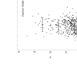
Figure 5: Color–magnitude diagram for all the 522 stars in the control field regions. The open circles represent sources with $(J-K)<0.5$ mag (the blue group, described in Sec. 3.1) and the filled circles represent sources with $(J-K)>0.5$ mag (the red group). The open squares and the error bars represent the mean and the dispersion, respectively, of the $(H-K)$ color in the (2 magnitudes wide) bins centered at $K=$ 9, 11, and 13.

Because of dust extinction, stars that will be detected through the increasingly denser regions of L977 can only be the brighter background stars. It is important then to know how the mean $(H-K)$ color and dispersion will vary with $K$ brightness as this variation might affect the correct determination of extinction from color excesses. To search for such possible variation we present in Figure 5 the color–magnitude diagram for all the stars in the control fields. The open circles represent sources with $(J-K)<0.5$ mag (the blue group, described in Sec. 3.1) and the filled circles represent sources with $(J-K)>0.5$ mag (the red group). To evaluate how the mean $(H-K)$ color and dispersion vary as a function of $K$ brightness we binned the data in $K$ (2 magnitudes bins) and determined the mean $(H-K)$ color and dispersion for each bin. This mean $(H-K)$ color and dispersion is represented in Figure 5 as the open squares and the error bars, respectively. We conclude that while the dispersion is essentially the same for all bins there is a slight increase in the mean $(H-K)$ color from fainter to brighter magnitudes. This is caused by the larger number of red sources (most likely red background giants; see Appendix) that populate the bright end of the color–magnitude diagram. Nevertheless, this increase ($\sim$ 0.05) is less than half the average dispersion ($\sim$ 0.13) and has a negligible effect on the determinations of extinction.

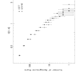
Figure 6: Frequency distribution of detected background stars through L977 and IC 5146 molecular cloud. The similarity in the shape of both distributions suggests a similar physical structure for these two clouds.

In Figure 6 we plot the frequency distribution of A_V’s derived toward L977. For comparison we also plot the distribution of A_V’s for IC 5146 using the data of Lada et al. (1994). The systematic offset between both distributions is caused by the richer background of L977 at lower galactic latitudes. The shape of these distributions is a function of both the detailed distribution of matter within the cloud and the detection limits of the infrared survey at high extinctions. The distributions in both clouds fall off steeply with increasing extinction in a fashion roughly consistent with a power–law. This indicates that the amount of material at high extinctions is relatively small in both these filamentary dark clouds. At high extinctions the steepness of the distribution is enhanced by the inability to detect heavily reddened faint stars imposed by the sensitivity of the NIR survey. Since the sensitivity of both surveys is the same, the similarity of the shapes of the extinction frequency distributions suggests that both L977 and IC 5146 are characterized by a similar intrinsic structure, i.e., a comparable proportion of high column density to low column density gas. In Section 4.5 of this paper we will model this frequency distribution for various clouds configurations.

To characterize the large–scale global structure of the cloud we spatially convolve the individual pencil–beam measurements (which represent a random spatial sampling of the cloud extinction) with a square filter 90^′′ in size and produced an ordered map of the extinction uniformly sampled at the Nyquist frequency. The map is shown in Figure 7 superposed on a digitized POSS red plate of the region. The 1$\sigma$ confidence level on the derived extinction measurements toward individual stars is set by the rms dispersion in the $(H-K)$ color of background stars measured in the control fields (Figure 3) and is equal to $\sim$ 2 magnitudes of visual extinction. The 1$\sigma$ confidence level on a map pixel is nevertheless $\sim$ 1 magnitude (see discussion in Section 4.6). Stars suspected to be foreground to the cloud (see next section) were removed from the database. Contours start at 4 visual magnitudes of extinction (4$\sigma$) and increase in steps of 2 magnitudes up to 24 magnitudes of visual extinction. The discontinuity near the bright star SAO 050355 is due to lack of one SQIID field in our data. We decided not to take this field as a precautionary measure since this SAO star, a M3 star (Neckel 1974) with an estimated $K=$ 3.8 mag, would potentially affect the SQIID detector. The overall shape of the map correlates well with the shape of the more opaque regions of the molecular cloud (see Figure 7).

4.2 Distance Determination

The only reference in the literature regarding the distance towards L 977 appears in Dobashi et al. (1994) ¹³CO survey. These authors estimate a distance of 800 pc from association to nearby astronomical objects with known distances. We used the Wainscoat et al. (1992) infrared model of the Galaxy to determine the expected number of foreground stars seen toward the opaque regions of L977 and independently determined a distance to this cloud. The molecular cloud can be used as a wall to discriminate between foreground/background stars as foreground stars are easily detected against the regions of high extinction. We searched for these stars in regions that presented an average extinction above 8 magnitudes (the central region of the L977 filament, $\sim$ 36 arcmin²) and compared the number of stars with derived extinctions A${}_{V}<2$ mag (5 stars) with the expected number of foreground stars from the galactic model. The $K-$band surface density of stars of the control fields was used to calibrate the galactic model. In Figure 8 we present the expected number of foreground stars toward the denser (A${}_{V}>$ 8 mag) regions of L977 as a function of distance. We estimate a distance to L977 molecular cloud of 500 $\pm$ 100 pc.

Extra information regarding a lower limit to the distance to L977 can be obtained from studied bright stars clearly foreground to the cloud. There are two such bright stars seen in projection against the molecular cloud complex:

1. Less than 1^∘ North of L977 (in front of L988, a molecular cloud associated in projection and velocity with L977) lies SAO 033091 (HR 8072), a K0III star with a visual magnitude of m${}_{V}=$ 6.37 (Breger 1968, Strassmeier et al. 1994). This star was observed with the astrometric satellite HIPPARCOS (Perryman et al. 1997) and an accurate distance of 119$\pm$8 pc was derived from trigonometric parallax (a spectrophotometric parallax would have given a distance $\sim$ 150 pc). The distance determined by HIPPARCOS can be taken as a conservative lower limit of the distance to L977.

2. The second bright star, not as well studied as SAO 033091, is seen in projection against L977 (SAO 050355, see Figure 1) . It was classified as a M3 star by Neckel (1974) but there is no information available on its luminosity class. If we assume a main-sequence, giant, or supergiant luminosity we can determine a distance of d${}_{V}=\,\,\sim 8$ pc, d${}_{III}=\,\,\sim 580$ pc, or d${}_{I}=\,\,\sim 4800$ pc respectively to this star. In any case the derived extinction is negligible which puts this star in the foreground of L977. We can readily dismiss the derived distance of 4800 pc: 1) at this distance we would be seeing this star at least through two of the Galaxy’s spiral arms ($l=90$^∘, $b=2$^∘) which is not compatible with the negligible extinction measured towards this star and 2) at this distance there would be no contrast to distinguish the shape of L977 against the background field due to foreground stars which is clearly not the case. The other two derived distances cannot be dismissed but while d${}_{V}=\,\,\sim 8$ pc would bring no further constraints to this discussion, the one determined for the giant star case (580 pc) is still consistent, within the uncertainties, with a distance of 500 $\pm$ 100 pc derived from the galactic model.

The uncertainty associated with the distance determination will be the largest source of systematic error in the derived properties of L977. We will assume 500pc as the distance to L977 throughout this paper.

4.3 Derived Mass

A precise mass determination (and accurate if not for the uncertainty associated with the distance determination) can then be obtained for L977 through spatial integration of the extinction map in Figure 7. Using the standard gas–to–dust ratio (i.e., N(H + H₂) = 2 $\times$ 10²¹ cm^-2 mag^-1; Lilley 1955, Bohlin et al. 1978), and typical mass fractions ($\sim$ 63% H₂, $\sim$ 36% He, $\sim$ 1% dust; e.g., Rohlfs & Wilson 1996) we derive a mass of the surveyed area of the cloud: $M_{L977}=(660\pm 30)\ (D/0.5kpc)^{2}\$ M_⊙  where $D$ is the true distance to this molecular cloud.

4.4 The $\sigma_{disp}$ versus A_V Relation

Our ordered map of the distribution of extinction in L977 provides useful information about the overall large–scale structure and distribution of mass in the cloud. However this is done at the expense of angular resolution. Since each extinction measurement is made along an individual pencil–beam through the cloud the observations represent a random, but highly undersampled map of extinction made at infinitely high angular resolution. One of the most interesting results of the first application of the NICE method to a dark cloud was the demonstration that useful information concerning cloud structure on small angular scales could be derived from the randomly sampled extinction measurements. Lada et al. (1994) showed that the relation between $\sigma_{disp}$, the dispersion of extinction measurements within a square map pixel, and A_V, the mean extinction derived for the map pixel, can be used to characterize cloud structure on scales smaller than the resolution of the map (i.e., the size of the map pixels). In IC 5146 Lada et al. (1994) found that $\sigma_{disp}$ increased in a systematic fashion with increasing A_V. At the same time the dispersion in this relation was also found to increased with A_V. Through modeling, this relation was found to be related to the form of the distribution of the small–scale cloud structure. In Figure 9 we present this same relation for L977. The same trend observed in IC 5146 is found for L977. A least–squares fit over the entire data set returns:

$$\sigma_{disp}\>\,=1.93\pm 0.11+(0.40\pm 0.02)\,A_{V}\,\,\,\,(mag)$$

The slope of the relation is virtually the same as that found in the IC 5146 study ($0.40\pm 0.01$).

The increase in the value of the intercept (from 0.73 in IC 5146 to 1.93 in L977) is solely related to the higher dispersion in the colors of background stars in the present study (Lada et al. 1994). We note, however, that this new data set (L977) is not as robust as the IC 5146 data set since there are not as many measurements at high extinction. This is related to the fact that the total area surveyed in the L977 study is smaller than that in IC 5146. Apparently, the same general behavior of the $\sigma_{disp}$ versus A_V relation is observed for L977. As was shown by Lada et al. (1994), this indicates that significant structure must be present down to scales smaller than the extinction map resolution, and moreover the dust cannot be distributed uniformly or in discrete high–extinction clumps on scales smaller than our resolution (0.22pc). In a recent paper, Padoan, Jones, & Nordlund (1997) found that the form of the observed $\sigma_{disp}$ versus A_V relation is consistent with cloud structure models characterized by supersonic random motions. However, it is not clear whether the shape of the $\sigma_{disp}$ versus A_V relation is due to random spatial fluctuations in the cloud structure or to systematic, unresolved gradients in the distribution of extinctions (e.g., Thoraval, Boissé, & Duvert 1997). Higher sensitivity and angular resolution observations are needed to resolve this issue.

4.5 Modeling and Density Structure

It is possible to predict the frequency distribution of detected background stars through the target cloud as presented in Figure 6. The decrease in the observed number of background stars for increasing cloud depth results from the combined effect of two causes: 1) extinction of the faintest stars in the background luminosity function to below the limits of detection and 2) the large–scale distribution of mass, as traced by dust extinction, inside the molecular cloud. The existence of a rising luminosity function determines that for the same detection limit only the intrinsically brighter (and fewer) stars can be detected as dust extinction (e.g., A_V) increases. The way dust extinction is distributed inside the cloud will also affect the final shape of the observed frequency distribution.

We constructed Monte Carlo models with different cloud configurations to mimic the infrared data and predict the shape of the frequency distribution of stars detected through the cloud. Because of the cloud’s filamentary nature we adopted a cylindrically symmetric synthetic cloud with a finite radius $R$. For every model the distribution of mass inside the model cloud was characterized by a density profile of the form $\rho\,(r)=\rho_{0}({r\over r_{0}})^{-\alpha}$ with $\alpha=$ 0, 1, 2, 3, and 4 where $r$ is the orthogonal distance from the major axis of the cylindrical cloud. The density profile was integrated to produce a column density (or visual extinction) profile for the synthetic cloud, i.e.:

$$A_{V}(p)=10^{-23}\times\rho_{0}r_{0}^{\alpha}\times\int\limits_{0}^{S}(s^{2}+p^{2})^{-{\alpha\over 2}}ds\ \,\,(mag)$$

where

$$S=(R^{2}-p^{2})^{1\over 2}$$

and where $p$ is the projected distance of the line–of–sight from the major axis of the cloud, $s$ is the distance through the cloud along the line–of–sight and $\rho_{0}$ and $r_{0}$ the appropriate scaling constants for the density distribution. This column density profile was then scaled to fit the data: the total radius of each cloud model was taken as the one that best reproduced the observed contrast from the highest measurements of extinction (A${}_{V}\sim 40$ mag, at $\sim$ 40^′′ from the center of the filament) to the lowest (1$\sigma$) measurements (A${}_{V}\sim 2$ mag, at $\sim$ 275^′′ from the center of the filament).

We then constructed synthetic luminosity functions for the background population from randomly sampling the $K$ luminosity function of the Control Fields. Stars from the synthetic background luminosity function were randomly assigned a projected distance from the center of the cloud. This assumes a uniform spatial distribution of background stars which is supported by the similarity between the East and West Control Fields (see Section 3). Next, the corresponding extinction A_V, for a given density structure model, was assigned to each star. Noise, simulating extinction measurement errors (see next Section) was also added to each star’s extinction value. The extincted brightness of each star was then calculated. Stars whose extincted brightness was less than the limiting sensitivity of our SQIID survey were rejected from further consideration. One realization was completed when the total number of extincted detectable stars (with A${}_{V}\leq 2$) reached the observed number: 889. To mimic the effects of the foreground stellar population we randomly assigned a zero extinction (plus noise) to five stars (see Section 4.2) in each realization. A total of 1000 realizations for each cloud model ($\alpha=$ 0, 1, 2, 3, and 4) were performed. To compare the different model clouds and the observed frequency distribution the resulting extinction (unbinned) distribution from each individual realization was compared to the observed (unbinned) distribution via the KS test.

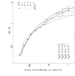
Figure 10: Observed frequency distribution of extinction measurements for L977 and the predictions from clouds models with density structures $\rho\,(r)\propto r^{-\alpha}$ having $\alpha=$ 1 (dashed line), 2 (solid line), 3 (dotted line), and 4 (dashed–dotted line). The represented predictions correspond to the average of the 1000 realizations done for each cloud model. The average KS probability for all realizations in each model is presented.

In Figure 10 we present the comparison between the observed frequency distribution of extinction measurements and the predictions from clouds models with density structures having $\alpha=$ 1 (dashed line), 2 (solid line), 3 (dotted line), and 4 (dash–dotted line). The represented predictions correspond to the average of the 1000 realizations done for each cloud model. Both the data and the results from the models are binned in 2 mag wide bins. The average KS probability for all realizations in each model was p${}_{KS}\,(\alpha=1)\approx 10^{-3}$, p${}_{KS}\,(\alpha=2)\approx 0.43$, p${}_{KS}\,(\alpha=3)\approx 0.03$, and p${}_{KS}\,(\alpha=4)\approx 10^{-3}$ with rms dispersions of 10^-2, 0.24, 0.05, and 10^-2 respectively. The constant density case, $\alpha=0$, predicts a slowly increasing frequency distribution with a zero probability of being, together with the observed distribution, randomly drawn from the same parent distribution. This model cloud is not represented on Figure 10 for the sake of clarity. Our Monte Carlo simulation suggests that the large–scale distribution of matter inside L977 is most consistent with a density structure $\rho\,(r)\propto r^{-2}$. We note that an isothermal cylinder has a density structure $\rho\,(r)\propto r^{-4}$ (Ostriker 1964).

In Figure 11 we present the averaged extinction profile of the southern portion of L977 where the center to edge contrast in extinction is the highest. Each point in this figure represents the average extinction along the North–South direction of 7 adjacent extinction map pixels covering a declination of $\sim 5$ arcmin on the southern part of the NIR survey, where the filament is roughly aligned to the North-South direction. The error bars represent the rms dispersions in the average of the pixels. The “bump” around 300 arcsec is caused by a small secondary condensation within L977. The dotted lines are column density profiles corresponding to radial density laws $\rho\,(r)\propto r^{-\alpha}$, for $\alpha=$0, 1, 2, and 3. The best fit between the observed radial profile and the various model profiles occurs for a $\rho\,(r)\propto r^{-2}$ density structure. The 1$\sigma$ uncertainty in the averaged extinction measurements is now A${}_{V}\sim 0.3$ mag. We conclude from our Monte Carlo simulation and from the observed radial profile of the cloud that the distribution of matter inside L977 between 2 $<$ A_V $<$ 40 mag (or 1 $<$ $r$ $<$ 0.1pc) is consistent with a density profile of $\rho\,(r)\propto r^{-2}$.

We do not expect the density in the inner part of L977 to reach infinity as $r\rightarrow 0$. Clearly a break at some small $r_{0}$ ($r_{0}$$\;\buildrel<\over{\sim}\;$0.1pc; from Figure 11) must occur. With the present data we cannot probe the very inner part of L977 because we do not detect stars through it. In fact, even with new and more sensitive near–infrared arrays this will not be an easy task since the probability of having a fairly bright background star within a smaller solid angle (the denser regions of the cloud) is also increasingly small.

4.6 The Effect of Galactic Latitude on the NICE Method

It was a goal of this article to analyze the effects of a richer but more complicated background of field stars — at lower galactic latitude — on the application of the NICE method. An extensive discussion on the limitations and uncertainties in this method is given by Lada et al. (1994). Here we will only be concerned about the limitations that result from applying the NICE method to low Galactic latitude molecular clouds by comparing the previous study (IC 5146, $b=-5$^∘) with the present one ($b=2$^∘).

The angular resolution of the dust extinction map is limited by the surface density of stars detected through the target cloud at both the $H$ and $K-$bands. For the same detection limit it is clear that better resolution, hence more complete information on the small–scale spatial distribution of dust, can be obtained for clouds that lie in the foreground of rich star fields close to the Galactic plane. On the other hand it was unclear before the present study what was the contribution of distant luminous giant stars, suffering extraneous extinction, to the increase in the dispersion of the mean ($H-K$) color of control field stars at these low Galactic latitude fields. The NICE method is sensitive to this mean color since it assumes that the intrinsic $(H-K)$ color of stars behind the cloud is accurately represented by the mean color of the control fields. A successful application of the method requires, to first order, the dispersion on the mean ($H-K$) color for the control fields to be significantly smaller than the observed range in $(H-K)$ colors for stars seen through the target cloud.

A direct consequence of observing at low Galactic latitudes is an appreciable increase in the mean and dispersion of the observed $(H-K)$ (and ($J-H)$) color of stars:

$$<(H-K)>_{IC5146}\>\,=0.13\pm 0.08\>\,mag\,\,\,\,\,\,\,\,(b=-5^{\circ})$$

$$<(H-K)>_{L977}\>\,=0.20\pm 0.13\>\,mag\,\,\,\,\,\,\,\,\,(b=2^{\circ})$$

While the value of the mean observed $(H-K)$ color will function as a zero–point for the derived extinction measurements with the NICE method, the dispersion in this value — $\sigma(H-K)_{intrinsic}$ — sets the threshold (1$\sigma$ confidence level) above which extinctions toward background stars can be reliably measured. The observed increase in dispersion, caused by distant reddened giants detected at low Galactic latitude, is going to raise this threshold.

For the IC 5146 study the threshold value was $\sim$ 1 magnitude of visual extinction and it was similar to the measurement uncertainty on a pixel of the derived extinction map:

$$\sigma_{pixel}\ =\ {15.9/N}\sqrt{\Sigma_{i=1}^{N}(\sigma(H-K)^{2}_{i}+\sigma(H-K)^{2}_{intrinsic})}\,\,\,\,\,\,\,\,(mag)$$

where $\sigma(H-K)_{i}$ is the photometric error in the derived color for a star in a given map pixel and N is the number of stars in that pixel. For the L977 study the larger value of $\sigma(H-K)_{intrinsic}$ raises the threshold to $\sim$ 2 magnitudes of visual extinction while the uncertainty in the extinction map is still $\sim$ 1 magnitude of visual extinction. The uncertainties on a map pixel are similar in both studies because the average number of stars inside each pixel map is now 8 (instead of 5 for the IC 5146 study) which compensates for the larger $\sigma(H-K)_{intrinsic}$ observed in the present study.

We conclude that the consequence of applying the NICE method at low Galactic latitudes is an increase of as much as a factor of 2 in the 1$\sigma$ confidence level in the derived extinction measurements toward background stars. This is directly related to the detection at low galactic latitudes of a large number of giant stars along the plane of the Galaxy affected by random, unrelated, amounts of extinction and affects somewhat the method’s aptitude to address small–scale cloud structure (e.g., the increase in random dispersion around the $\sigma_{disp}$ versus A_V relation). Nonetheless, and because of the comparatively higher number of stars detected at these very low galactic latitudes $(b=2^{\circ})$ , the capacity of the method to study the large–scale distribution of dust in a molecular cloud is essentially the same as an application of the method at the same galactic longitude but at a galactic latitude $(b=-5^{\circ})$ free from “contamination” of distant giant stars. The NICE method remains a powerful method for mapping the distribution of dust through a molecular cloud.

5 Summary

We applied the NICE method to the L977 molecular cloud. The main findings of this paper are as follow:

• We use measurements of the near–infrared color excess and positions of the 1628 brightest stars in our survey to directly measure dust extinction through the cloud following the method described by Lada et al. (1994).

• We construct a detailed map of the distribution of dust extinction of L977 molecular cloud at an effective angular resolution of 90^′′ by spatially convolving the individual extinction measurements. We derive a distance of 500 $\pm$ 100 pc towards this cloud via a comparison of source counts with predictions of a galactic model. From integration of the extinction map we determine the total mass of the cloud to be $M_{L977}=(660\pm 30)\ (D/500pc)^{2}$ M_⊙ where $D$ is the true distance to the cloud.

• We find a correlation between the measured dispersion in our extinction determinations and the extinction which is very similar to that found for the dark cloud IC 5146 in a previous study. We interpret this as evidence for the presence of structure on scales smaller than the 90^′′ resolution of our extinction map.

• To further investigate the structure of the cloud we construct the frequency distribution of the 1628 individual extinction measurements in the L977 cloud. The shape of the distribution is similar to that of the IC 5146 cloud suggesting that both clouds are characterized by a similar structure. Monte Carlo modeling of this distribution suggests that between 2 $<$ A_V $<$ 40 mag (or roughly 1 $<$ $r$ $<$ 0.1 pc) the material inside L977 is characterized by a density profile $\rho\,(r)\propto r^{-2}$. Direct measurement of the radial profile of a portion of the cloud confirm this result.

• From comparison between the colors of stars seen through L977 and color of stars in the control fields we derive the slope of the near–infrared extinction law to be $E(J-H)/E(H-K)=1.6\pm 0.1$.

• At the lower galactic latitude of L977, we find both the mean and dispersion of the infrared colors of field stars to be larger than observed toward IC 5146. This produces an increase of about a factor of 2 in the minimum or threshold value of extinction that can be reliably measured toward L977 with this technique. Nevertheless the accuracy in an extinction map pixel is not significantly different toward L977 due to the increased number of field stars at this latitude. We also find an increase in the number of detected giant stars at the low galactic latitude of the survey by almost a factor of two. Most of these excess stars suffer extraneous extinction and are probably red giants seen along the disc of the Milky Way up to distances $\sim$ 15 kpc and reddened by unrelated background molecular clouds along this direction of the Galaxy. We discuss a possible application of this observable to galactic structure studies on the plane of the Galaxy.

Appendix A The Effect of Galactic Latitude on NIR Color–Color Diagrams

A comparison between L977 control fields ($b=$ 2^∘) with control fields at essentially the same Galactic longitude but not as close to the Galactic plane (IC 5146 molecular cloud, $b=-$5^∘, Lada et al. 1994) reveals significant differences. In Figure A1 we present the color–color diagrams for both regions. The contours represent surface density of stars in the [($J-H),(H-K)$] color–color plane. Contours are 30% (2$\sigma$), 45%, 60%, 75%, and 90% of the maximum number of stars/mag² and were obtained by sampling the color–color plane at Nyquist frequency with a square filter with a resolution equal to the average photometric error (0.1 mag) in both samples. The resolution is represented by the square box at the upper right corner of both diagrams. The dwarf and giant sequence (solid line) and the reddening vector (dashed line) are as in Figure 3. Both IC 5146 and L977 control fields regions show a similar, but not identical, bimodal distribution of sources on the color–color plane, i.e., a blue group centered at the color of a mid G main–sequence star and a red group centered at the color of an early K giant/main–sequence star. For the SQIID detection limit the blue group is dominated by F main-sequence stars located at distances smaller than 1 kpc while the red group is dominated by early K giant stars located at a broad range of distances that can surpass 15 kpc (Alves 1998).

Within the sampling resolution the blue group seen in the L977 control fields is similar to the one in IC 5146 control fields. This is not surprising since both groups likely consist of a similar population of local main-sequence stars. If relevant at all, the somewhat higher scatter observed in the L977 blue group can be due to higher interstellar extinction towards this direction which lies closer to the plane of the Galaxy. A significant difference in both diagrams is revealed in the comparison of the red groups. The center of the L977 red group is not only displaced along the reddening vector when compared to IC 5146 red group but its overall shape is changed: the uniform distribution of stars around a preferred point in the color–color plane for the IC 5146 red group is replaced by an elongated distribution along the reddening vector for the L977 red group, indicating the presence of additional differential extinction for this population of stars. Also, the fraction of sources belonging to the red group (essentially the ratio [#giants/#main–sequence stars]) detected in the IC 5146 control fields is 37% while for L977 this fraction rises to 56%, almost a factor of two higher.

There is a clear “contamination” by reddened background giants in our $JHK$ color–color diagram closer to the Galactic plane. Giant stars are easily detected even at very large distances because: 1) they are luminous NIR emitters (M${}_{K}\sim-3$ mag and T $\sim$ 4000 K for an early K giant), 2) the opacity of the plane of the Galaxy at these wavelengths (1.25 to 2.2 $\mu$m) is modest, and 3) being the evolved counterparts of Sun–like stars, they are abundant. These facts alone do not explain the observed differences for the two fields. However, for low Galactic latitudes (as it is the case for the L977 control fields) we are basically observing along the Galactic disk virtually detecting giants to its edge. This can explain the observed increase in the ratio [#giants/#main–sequence stars] — this increase is in itself a measure of the relative distribution perpendicular to the plane of the giant population. Moreover, the farther a detected giant is along the plane the more likely it is to be affected by extinction. This is most probably the cause of the displacement and scatter along the reddening vector for the red group in the L977 control fields color–color diagram in Figure A1. The similarity between L977 control fields East and West (Figure 3), separated by 1^∘ in the sky, supports this idea by suggesting that the observed effect is characteristic of this part of the Milky Way.

Although the increase in the dispersion of the mean color of background stars is a nuisance in the present study there are obvious fruitful applications of this quantity to galactic structure studies along the plane of the galaxy. Classical galactic structure studies have always been severely hampered and confined to a few kpc around the Sun by the high opacity of the galactic plane that concealed from direct observation the regions where nearly all the luminous galactic mass is located. We note that the NIR is the wavelength of choice for this kind of study because of its comparative insensitivity to: 1) dust extinction, and 2) dust emission that begins to dominate at wavelengths longer than 5 $\mu$m. Moreover, the $JHK$ color–color diagram is a good discriminator of distant giant stars at low Galactic latitudes, as it is shown in Figure A1, hence a powerful tool to address galactic structure questions at the optically inaccessible low galactic latitudes, e.g., the large scale distribution of dust along the galactic plane, or the structure of the Galaxy’s outer disk.

Figure 1: Finding chart for L977. The area surveyed in the 3 NIR bands is represented as the central square overlaid on the Digitized Sky Survey red POSS plate. The L977 molecular cloud is readily seen as the zone of obscuration inside this square and seen against the rich star field that characterizes this region of the galaxy. The boxes to the East and to the West of L977 define the regions where the East and West control fields were taken. They are spatially separated in the sky by 1 degree ($\Delta l=0.7$^∘, and $\Delta b=0.8$^∘).

Figure 2: The photometric errors in the colors ($(J-H)$ open triangles; $(H-K)$ filled triangles) as a function of magnitude $(H)$ for stars observed toward L977.

Figure 3: Near–infrared ($JHK$) color–color diagrams for East and West control field regions. Also plotted as a solid line on both color–color diagrams are the locus of points corresponding to unreddened main sequence and giant stars (Koornneef 1983). The two parallel dashed lines define the reddening band for both main sequence and giant stars and were taken from Rieke & Lebofsky (1985). The typical photometric error for a 14^th $K$ magnitude star — roughly a 10 sigma detection — is displayed in the upper corner of both diagrams. The surface density of detected sources in the $JHK-$bands for the East control field region ($\Sigma_{E}$) is 4% higher than in the West control field region ($\Sigma_{W}$) — 2.6 against 2.5 stars per square arcmin — most likely due to the fact that the East control field region is almost 1^∘ closer to the Galactic plane. The mean $(H-K)$ and $(J-H)$ colors and dispersions for the two regions are, nevertheless, virtually the same. See text for full discussion.

Figure 4: Near–infrared ($JHK$) color–color diagram for the L977 field defined in Figure 1 by the central square region. The main sequence and giant locus, the reddening vector, as well as the photometric errors are the same as in Figure 2. The displacement in this diagram caused by 5 magnitudes of extinction is represented by the solid line to the left of the reddening vector. The ten most deviant sources scattered around the reddening vector were all found to be very close to the 10 sigma detection limit.

Figure 7: L977 dust extinction map derived from the infrared $(H-K)$ observations. Contours start at 4 visual magnitudes of extinction (4$\sigma$) and increase in steps of 2 magnitudes up to 24 magnitudes of visual extinction. The effective resolution of the map is 90^′′ (0.22pc at an estimated distance of 500 pc). The contours are overlaid on the digitized POSS red plate. The overall shape of the map correlates well with the shape of the more opaque regions of the molecular cloud. The discontinuity near the bright star SAO 050355 (a M3 star) is due to lack of one SQIID field in our data, not taken to avoid potential detector damage.

Figure 8: Expected number of foreground stars toward the denser regions ($\sim$ 36 arcmin²) of L977 as a function of distance. Five foreground stars were identified in the NIR survey toward these regions.

Figure 9: The relation between $\sigma_{disp}$, the dispersion in the extinction measurements, with visual extinction A_V. Also plotted is the least–squares linear fit to the data over the entire range of extinction. The same general behaviour is observed in the IC 5146 study (Lada et al. 1994).

Figure 11: Averaged radial profile of L977. The “bump” around 300 arcsec is caused by a small secondary condensation within L977. The dotted lines correspond to radial density profiles $\rho\,(r)\propto r^{-\alpha}$, for $\alpha=$0, 1, 2, and 3. The upper distance scale assumes a distance of 500pc to L977.

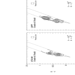
Figure A1: a) and b) Near–infrared ($JHK$) color–color diagrams for IC 5146 control fields (IC 5146 molecular cloud, $b=$-5^∘, Lada et al. 1994) and the L977 control fields ($b=$ 2^∘). The contours represent surface density of stars in the [($J-H),(H-K)$] color–color plane. Contours are 30% (2$\sigma$), 45%, 60%, 75%, and 90% of the maximum number of stars/mag² and were obtained by sampling the color–color plane at Nyquist frequency with a square filter with a resolution equal to the average photometric error in both samples (0.1 mag). The dwarf and giant sequence (solid line) and the reddening vector (dashed line) are as in Figure 2. Note the effects of the Galactic plane on the bimodal distribution of sources in the color–color plane.

References

- (1) Alves, J. 1998, PhD Thesis
- (2) Barsony, M., Kenyon, S., Lada, E. & Teuben, P. 1997, ApJS, 112, 109
- (3) Bessel, M., & Brett, J. 1988, PASP, 100, 1134
- (4) Bohlin, R. C., Savage, B. D. & Drake, J. F. 1978, ApJ, 224, 132
- (5) Breger, M. 1968, AJ, 73, 84
- (6) Cardelli, J.A., Clayton, G.C., & Mathis, J.S. 1989, ApJ, 345, 245
- (7) Dobashi, K., Bernard, J., Yonekura, Y., & Fukui, Y. 1994, ApJS, 95, 419
- (8) Elias, J. H., Frogel, J. A., Matthews, K. & Neugebauer, G. 1982, AJ, 87, 1029
- (9) Jenkins, E. B. & Savage, D. B. 1974, ApJ, 187, 243
- (10) Jones, T.J., & Hyland, A.R. 1980, MNRAS, 192, 359
- (11) Kenyon, S.J., Lada, E.A., & Barsony, M. 1998, AJ, 115, 252
- (12) Koornneef, J. 1983, A&A, 128, 84
- (13) Kramer, C., Alves, J., Lada, C.J., Lada, E.A., Sievers, A., Ungerechts, H., & Walmsley, M. 1998, in preparation
- (14) Lada, C.J., Lada, E.A., Clemens, D.P., & Bally, J. 1994, ApJ, 429, 694
- (15) Lilley, A. E. 1955, ApJ, 121, 559
- (16) Lynds, B. 1962, ApJS, 7, 1
- (17) Martin, P.G. & Whittet, D.C. 1990, Apj, 357, 113
- (18) Mathis, J. 1990, ARAA, 28, 37
- (19) Nagy, T. 1979, in “Documentation for the machine-readable version of Lynds’ Catalogue of Dark Nebula”, NASA document R-SAW-7/79-13
- (20) Neckel, H. 1974, A&AS, 18, 169
- (21) Ostriker, J. 1964, ApJ, 140, 1056
- (22) Padoan, P., Jones, B., & Nordlund, A. 1997, ApJ, 474, 730
- (23) Perryman, M. A. C. 1997, A&A, 323, L49
- (24) Press, W.H., Flannery, B.P., Teukolsky, S.A., & Vetterling, W.T. 1992, in “Numerical Recipes, The Art of Scientific Computing”, Cambridge, Cambridge
- (25) Rieke, G.H., & Lebofsky, M.J. 1985, ApJ, 288, 618
- (26) Schneider, S., & Elmegreen, B.G. 1978, ApJS, 41, 87
- Stetson (1987) Stetson, P. 1987, PASP, 99, 191
- (28) Strassmeier, K.G., Handler, G., Paunzen, E., & Rauth M. 1994, A&A, 281, 855
- (29) Thoraval, S., Boissé, P., & Duvert, G. 1997, A&A, 319, 948
- (30) Wainscoat, R.J., Cohen, M., Volk, K., Walker, H.J., Schwartz, D.E. 1992, ApJS, 83, 111
- (31) Whittet, D.C., Martin, P.G., Fitzpatrick, E.L., & Massa, D. 1993, ApJ, 408, 573