Observational Implications of Axionic Isocurvature Fluctuations

Abstract

The axion is the most attractive candidate to solve the strong CP problem in QCD. If it exists, the inflationary universe produces axion fluctuations which are mixtures of isocurvature and adiabatic fluctuations in general. We investigate how large isocurvature fluctuations are allowed or favored in order to explain observations of the large scale structure of the present universe. Generic flat universe models with mixed (isocurvature$+$adiabatic) density fluctuations are studied. It is found that the observations are consistent with the mixed fluctuation model if the ratio $\alpha$ of the power spectrum of isocurvature fluctuations to that of adiabatic fluctuations is less than $\sim 0.1$. In particular, the mixed fluctuation model with $\alpha\sim 0.05$, total matter density $\Omega_{0}=0.4$, and Hubble parameter $H_{0}=70$km/s/Mpc gives a very good fit to the observational data. Since the height of the acoustic peak in the angular power spectrum of the cosmic microwave background (CMB) radiation decreases significantly when the isocurvature fluctuations are present, the mixed fluctuation model can be tested in future satellite experiments. Ratios of the amplitude at the peak location to that at the COBE normalization scale for various models are given. Furthermore, we also obtain the amplitude of isocurvature fluctuations as a function of axion parameters and the Hubble parameter during the inflation. We discuss the axion fluctuations in some realistic inflation models and find that a significant amount of the isocurvature fluctuations are naturally produced.

I Introduction

The axion is a Nambu-Goldstone boson associated with spontaneous breaking of the Peccei-Quinn $U(1)$ symmetry which is introduced in order to solve the strong CP problem in quantum chromodynamics (QCD). The breaking scale $F_{a}$ of the Peccei-Quinn symmetry is stringently constrained by accelerator experiments, astrophysics and cosmology, and it should lie in the rage $10^{10}-10^{12}$GeV in standard cosmology. In particular, the upper limit is set by requiring that the cosmic density of the axion does not exceed the critical density of the universe. In other words, the axion should represent the dark matter of the universe if $F_{a}$ is $\sim 10^{12}$GeV, which makes the axion very attractive.

In the inflationary universe, quantum fluctuations of the inflaton field result in adiabatic density fluctuations with a scale-invariant power spectrum which would account for the large scale structure of the present universe. This natural generation of density fluctuations is one of successes of the inflationary universe. However, if the axion exists, another kind of fluctuations is produced in the inflationary universe. During inflation the axion has quantum fluctuations whose root mean square amplitude $\delta a$ is given by $H/(2\pi)$. ($H$ is the Hubble parameter during inflation.) The quantum fluctuations of the axion are stretched by the inflation and become classical. When the axion acquires a mass $m_{a}$ at the QCD scale, these axion fluctuations result in density fluctuations of the axion. However, since the axion is massless during inflation, axion fluctuations with wavelength larger than the horizon size do not contribute to the total density fluctuations. For this reason, such density fluctuations are called “isocurvature”. Therefore, if indeed the dark matter consists of axions, it has both adiabatic and isocurvature fluctuations and may play an important role in the structure formation of the universe.

In a previous work [1] the large scale structure formation due to the mixed (adiabatic $+$ isocurvature) fluctuations of the axion was studied with matter density parameter $\Omega_{0}=1$. It was found that the introduction of isocurvature fluctuations significantly reduces the amplitude of the power spectrum $P(k)$ of the density fluctuations, keeping $P(k)$ normalized by the COBE data. Since it is known that the cold dark matter (CDM) model with pure adiabatic density fluctuations and $\Omega_{0}=1$ predicts an amplitude of $P(k)$ that is too large on galaxy and cluster of galaxies scales, the mixed fluctuation model gives a better fit to the observations, although the shape $P(k)$ on larger scales does not quite fit the observations. Furthermore, it was also pointed out that the height of the acoustic peak in the angular power spectrum of the cosmic microwave background (CMB) radiation decreases when the isocurvature fluctuations are added, which can be tested in the future satellite experiments. Similar studies were also done in Refs. 2) and 3).

However, previous works deal with only restricted cosmological models (i.e. $\Omega_{0}=1$). It is well known that the shape of the power spectrum inferred from the galaxy survey [5] favors a low matter density universe. Therefore, in this paper we consider the structure formation with the mixed fluctuations in a generic flat universe (i.e. $\Omega_{0}+\lambda_{0}=1$, where $\lambda_{0}$ is the density parameter for the cosmological constant) and investigate how large isocurvature fluctuations are allowed or favored in order to explain the observations. The constraint on the amplitude of the isocurvature fluctuations is reinterpreted as a constraint on the Hubble parameter $H$ and the Peccei-Quinn scale $F_{a}$. We also study the cosmological evolution of the axion fluctuations in some inflation models. Among many inflation models, we adopt a hybrid inflation model and a new inflation model. In the hybrid inflation model, which is most natural in supergravity, we find that a significant amount of isocurvature fluctuations of the axion are naturally produced if $F_{a}\simeq 10^{15-16}$ GeV. We note that late-time entropy production may easily raise the $F_{a}$ up to $\sim 10^{16}$GeV. In the new inflation model, we also find that isocurvature fluctuations are produced with a canonically favored value of $F_{a}\sim 10^{12}$GeV without late-time entropy production.

In §II we investigate the structure formation with mixed fluctuations and compare the theoretical predictions with the present observations. The generation of isocurvature and adiabatic fluctuations of the axion is described in §III. We discuss some inflation models and isocurvature fluctuations of the axion in §IV. §V is devoted to conclusions and discussion.

Throughout this paper, we set the gravitational scale $\sim 2.4\times 10^{18}$GeV equal to unity.

II Comparison with observations

The density field of the universe is often described in terms of the density contrast, $\delta(\mbox{\boldmath$x$})\equiv\delta\rho(\mbox{\boldmath$x$})/\bar{\rho}=\left(\rho(\mbox{\boldmath$x$})-\bar{\rho}\right)/{\bar{\rho}},$ and its Fourier components $\delta_{k}=\frac{1}{V}\int d^{3}\mbox{\boldmath$x$}\ \delta(\mbox{\boldmath$x$})\exp\left(i\mbox{\boldmath$k$}\cdot\mbox{\boldmath$x$}\right),$ where $\bar{\rho}$ is the average density of the universe, $x$ denotes comoving coordinates, and $V$ is a sufficiently large volume. If $\delta(\mbox{\boldmath$x$})$ is a random Gaussian field as predicted by the inflation, then the statistical properties of the cosmic density field are completely contained in the matter power spectrum $P(k)\equiv V\langle|\delta_{k}|^{2}\rangle$, where $\langle\cdots\rangle$ represents ensemble average.

In general, the inflation predicts an adiabatic primordial spectrum, $P_{\rm ad}^{prim}(k)\propto k^{n_{s}}$, where $k$ is the wavenumber of perturbation modes, and $n_{s}$ a spectral index. In this paper, we set $n_{s}=1$ (the Harrison-Zeldovich spectrum), which is predicted in a large class of inflation models including hybrid inflation, new inflation, and the chaotic inflation models discussed in §IV. As for isocurvature perturbations, on the other hand, the primordial spectrum index is conventionally expressed in terms of entropy perturbations $S_{ar}\equiv\delta_{a}-{3\over 4}\delta_{r}$ as $S_{ar}(k)\propto k^{\tilde{n}_{s}}$, where $\delta_{a}$ and $\delta_{r}$ are density fluctuations of axion and radiation fields, respectively. Employing this definition, we can express the primordial power spectrum as $P_{\rm iso}^{prim}(k)\propto k^{\tilde{n}_{s}+4}$. We set ${\tilde{n}}_{s}=-3$, which corresponds to the Harrison-Zeldovich spectrum.

The primordial power spectrum is modified through its evolution in the expanding universe and the present power spectrum can be described as

$$P(k)=P_{\rm ad}+P_{\rm iso}=A_{\rm ad}kT_{\rm ad}^{2}(k)+A_{\rm iso}kT_{\rm iso}^{2}(k),$$ (1)

where $A_{\rm ad}$ and $A_{\rm iso}$ are normalizations of adiabatic and isocurvature perturbations, and $T_{\rm ad}(k)$ and $T_{\rm iso}(k)$ are transfer functions of adiabatic and isocurvature perturbations. Conventionally, the transfer function of the isocurvature perturbations is defined for the initial entropy perturbations. Therefore the present matter power spectrum may be written as $P_{\rm iso}=\tilde{A}_{\rm iso}k^{-3}\tilde{T}^{2}_{\rm iso}(k)$. For this definition, $\lim_{k\rightarrow\infty}\tilde{T}_{\rm iso}(k)=1$, while $\lim_{k\rightarrow 0}{T}_{\rm iso}(k)=1$ for Eq.(1). However, this definition makes direct comparison between adiabatic and isocurvature matter power spectra difficult. Therefore we employ Eq.(1) to define the amplitude and the transfer function for both adiabatic and isocurvature perturbations.

Here we define the ratio $\alpha$ of the isocurvature to the adiabatic power spectrum as [1, 6]

$$\alpha\equiv{A_{\rm iso}\over A_{\rm ad}}~{}.$$ (2)

It is well known that the transfer functions for adiabatic CDM models are essentially controlled by a single parameter, $\Gamma\equiv\Omega_{0}h$, [7] or more precisely, $\Gamma\equiv\Omega_{0}h(T_{0}/2.7K)^{-2}\exp(-\Omega_{B}-\sqrt{2h}\Omega_{B}/\Omega_{0})$. [8] Here $h$ is the present Hubble parameter normalized by $100$km s^-1 Mpc^-1, $T_{0}$ is the present cosmic temperature, and $\Omega_{B}$ is the ratio of the present baryon density to the critical density. From the galaxy survey Peacock and Dodds [5] estimated that $\Gamma\simeq 0.25\pm 0.05+0.32(n_{s}^{-1}-1)$.

In observational cosmology, the quantity $\sigma_{8}$, which is the linearly extrapolated rms of the density field in spheres of radius $8h^{-1}$Mpc, is often used to evaluate amplitudes of the density fluctuations. This is motivated by the fact that the rms fluctuation in the number density of bright galaxies measured in a sphere of radius of $8h^{-1}$Mpc is almost unity. [9] Employing the top hat window function, we obtain

$$\sigma^{2}_{8}=\frac{1}{2\pi^{2}}\int\frac{dk}{k}k^{3}P(k)\left.\left(\frac{3j_{1}(kr_{0})}{kr_{0}}\right)^{2}\right|_{r_{0}=8h^{-1}{\rm Mpc}}~{},$$ (3)

where $j_{1}$ is the spherical Bessel function.

Anisotropies of the cosmic microwave background radiation (CMB), $\delta T/T$, can be expanded as

$$\frac{\delta T}{T}(\mbox{\boldmath$\gamma$})=\sum_{\ell=2}^{\infty}\sum_{m=-\ell}^{m=+\ell}a_{\ell m}Y_{\ell m}(\mbox{\boldmath$\gamma$}),$$ (4)

where $Y_{\ell m}$ is a spherical harmonic function, and $\gamma$ denotes the direction in the sky. The temperature autocorrelation function (which compares the temperatures at two different points in the sky separated by an angle $\theta$) is defined as $\left\langle{\frac{\delta T}{T}(\mbox{\boldmath$\gamma$})\frac{\delta T}{T}(\mbox{\boldmath$\gamma^{\prime}$})}\right\rangle=\frac{1}{4\pi}\sum_{\ell}(2{\ell}+1)C_{\ell}P_{\ell}(\cos\theta),$ where $\gamma$$\cdot$ $\gamma^{\prime}$ $=\cos\theta$, and $P_{l}$ is the Legendre polynomial of degree $\ell$. The coefficients $C_{\ell}$ are the multipole moments:

$$(2\ell+1)C_{\ell}=\langle\sum_{m=-\ell}^{\ell}\left|a_{\ell m}\right|^{2}\rangle.$$ (5)

The predictions for the CMB anisotropies can be obtained by numerical integration of the general relativistic Boltzmann equations.

Since the isocurvature fluctuations are independent of adiabatic fluctuations and give different contributions to the CMB anisotropies, the CMB multipoles can be expressed as a linear combination of two components as

$$C_{\ell}(\alpha)=g(\alpha)C^{\rm ad}_{\ell}+h(\alpha)C^{\rm iso}_{\ell}~{},$$ (6)

where $C^{\rm ad}_{\ell}$ and $C^{\rm iso}_{\ell}$ are adiabatic and isocurvature components of CMB multipoles, respectively, and $g(\alpha)$ and $h(\alpha)$ are functions of $\alpha$. Note that $C^{\rm ad}_{\ell}=C_{\ell}(0)$ and $C^{\rm iso}_{\ell}=C_{\ell}(\infty)$. Employing the COBE normalization obtained from the 4-yr data, [10] which fixes $C_{10}$, i.e., $C_{10}=C^{\rm ad}_{10}=C^{\rm iso}_{10}$, we obtain $h(\alpha)=1-g(\alpha)$. Then we introduce a relative ratio between the isocurvature and adiabatic components at $\alpha=1$ as $f_{\ell}^{2}\equiv\left(1-g(1)\right)C^{\rm iso}_{\ell}/g(1)C^{\rm ad}_{\ell}$. In the large scale limit ($\ell\rightarrow 2$), this factor is almost $f_{\ell}\approx 6$, which is expected from the differences between Sachs-Wolfe contributions of adiabatic and isocurvature fluctuations. [11] On the COBE scale ($\ell\simeq 10$), however, $f_{\ell}$ is smaller than 6. Furthermore, for larger $\ell$, $f_{\ell}$ strongly depends on $\ell$ because the angular power spectra for the adiabatic and the isocurvature fluctuations differ greatly (see Fig.1). The precise value of $f_{10}$ depends on $\Omega_{0}$ and $h$. For example, $f_{10}^{2}\simeq 30$ for $\Omega_{0}=1$ and $h\gtrsim 0.6$, and it becomes smaller when $\Omega_{0}$ or $h$ becomes smaller. Using this factor $f_{\ell}$, we can write the ratio of the isocurvature to the adiabatic mode at arbitrary $\alpha$ as

$$f_{\ell}^{2}\alpha={\left(1-g(\alpha)\right)C^{\rm iso}_{\ell}\over g(\alpha)C^{\rm ad}_{\ell}}~{}.$$ (7)

Using the COBE normalization, we get $g(\alpha)=1/(1+f_{10}^{2}\alpha)$. Eventually, if we know the value of $f_{10}$, the COBE normalized pure adiabatic ($C^{\rm ad}_{\ell}$) perturbations, and isocurvature ($C^{\rm iso}_{\ell}$) perturbations, we can obtain the COBE normalization for any admixture of adiabatic and isocurvature perturbations as

$$C_{\ell}(\alpha)={C^{\rm ad}_{\ell}+f_{10}^{2}\alpha C^{\rm iso}_{\ell}\over{1+f_{10}^{2}\alpha}}~{}.$$ (8)

A similar argument can be applied to $\sigma_{8}$ as

$$\sigma_{8}(\alpha)=\sqrt{\frac{(\sigma^{\rm ad}_{8})^{2}+f_{10}^{2}\alpha(\sigma^{\rm iso}_{8})^{2}}{1+f_{10}^{2}\alpha}},$$ (9)

where $\sigma_{8}^{\rm ad}$ and $\sigma_{8}^{\rm iso}$ are the values of $\sigma_{8}$ normalized to COBE for the cases of pure adiabatic and pure isocurvature perturbations, respectively.

We can obtain $\sigma_{8}$ as a function of $\Omega_{0}$ from observations of the cluster abundance, since this abundance is very sensitive to the amplitude of the density fluctuations. Here we adopt the values of $\sigma_{8}$ which are obtained from the analysis of the local cluster X-ray temperature function: [12]

$$\sigma_{8}=(0.52\pm 0.04)\Omega_{0}^{-0.52+0.13\Omega_{0}}\quad({\rm for}\quad\Omega_{0}+\lambda_{0}=1).$$ (10)

In other analyses, [13, 14, 15] similar values for $\sigma_{8}$ have been obtained.

In Figs.2 and 3, we plot $\sigma_{8}(\alpha)$ as functions of $\Omega_{0}$ and $h$. The observed $\sigma_{8}$ mentioned above is also drawn as a region inside the two short dash - long dash lines. Furthermore, three dashed lines, corresponding to the shape parameters $\Gamma=0.2,0.25$, and $0.3$ from left to right, are drawn in the figures. From these figures, one can see that, for example, if $h\simeq 0.7$ and $\Gamma=0.25\pm 0.05$, the observed $\sigma_{8}$ is inconsistent with the COBE normalized predictions for $\alpha=0$. It is possible, of course, to fit the observation with $\alpha=0$ if $h\simeq 0.4(\Omega_{0}\simeq 0.6)$. However, small values of the Hubble parameter ($h\simeq 0.4$) seem unlikely from the recent observations, [16] which suggest $h=0.73\pm 0.06({\rm stat})\pm 0.08({\rm sys})$. Rather, $\alpha=0.04$ to $0.06$ give better fits for $h\simeq 0.7$. This fact is also seen in Fig.4 (left panel), where the power spectrum for $\alpha=0.05,\Omega_{0}=0.4$ and $h=0.7$ is shown together with observational data. [5] In Fig.4 we also plot the pure adiabatic power spectrum for $\Omega_{0}=0.3$ and $h=0.7$ for comparison (right panel). The values of $\Omega_{0}$ for both power spectra are chosen to satisfy Eq. (10) for $h=0.7$. It is clear that the mixed model ($\alpha\simeq 0.05$) gives a much better fit to the data obtained from the galaxy survey.

For each $\Omega_{0}$ and $h$, we can obtain the best fit values of $\alpha$, which are plotted in Fig.5. The three dashed lines correspond to $\Gamma=0.2,0.25$, and $0.3$, from left to right. One can see from this figure, for example, for $h=0.7$ and $\Gamma=0.25$, the best fit value of $\alpha$ to observations is $\alpha\simeq 0.05$. This figure also indicates that if $\Gamma=0.25\pm 0.05$, the observations of $\sigma_{8}$ require $\alpha\lesssim 0.1$. This is also seen in Fig.3.

In the above discussion, we see that $\alpha\sim{\cal O}(10^{-2})$ is consistent with observations of large scale structures. Let us examine what this value predicts. As mentioned earlier, the isocurvature fluctuations give different contributions to the CMB anisotropies than the adiabatic fluctuations. If one takes very large values of $\alpha$, the prominent acoustic peaks disappear, and only the Sachs-Wolfe plateau exists in the angular power spectrum. Therefore, we must investigate the height of the acoustic peak(s) predicted by our model.

In order to predict this height quantitatively, we introduce the peak-height parameter in the CMB anisotropy angular power spectrum defined by

$$\gamma\equiv\frac{\left.\ell(\ell+1)C_{\ell}\right|_{\ell=\ell_{\rm peak}}}{\left.\ell(\ell+1)C_{\ell}\right|_{\ell=10}},$$ (11)

where $\gamma,\ C_{\ell}$ and $\ell_{\rm peak}$ are all functions of $\alpha$. Here $\left.\ell(\ell+1)C_{\ell}\right|_{\ell=\ell_{\rm peak}}$ denotes the highest value, which is usually the value at the first acoustic peak. When $\alpha$ becomes larger, the height of the acoustic peak becomes lower. If the peak height becomes lower than the Sachs-Wolfe plateau, this peak-height parameter tends to be unity. In Fig.6, we plot this quantity. One can see that, for example, for $\alpha\simeq 0.05$, $\Omega_{0}=0.4$, and $h=0.7$, this ratio is about $\gamma\simeq 2$ - $3$.

In Fig.7, we plot the CMB angular power spectra normalized by the COBE for the cases $\alpha=0,\ 0.05$, and $\infty$. Also, in Fig.8, we plot the same angular power spectra, changing the cosmological parameters $\Omega_{0}$ and $h$. From these figures, one can see how much the height of the acoustic peak decreases when $\alpha$ is large.

Future satellite experiments such as MAP [17] and PLANCK [18] are expected to measure the CMB anisotropies with fine angular resolutions and detect the peak-height parameter. If this is done, our model can be tested by these observations.

III Fluctuations of axions

During the inflation, the axion experiences quantum fluctuations whose amplitude is given by

$$(\delta a(k))^{2}=\frac{H^{2}}{2k^{3}},$$ (12)

where $k$ is the comoving wavenumber and $H$ the Hubble parameter during the inflation. These fluctuations become classical due to the exponential expansion of the universe. After the axion acquires a mass at the QCD scale, the axion fluctuations lead to density fluctuations. The density fluctuations of axions are of an isocurvature type, because they are massless during the inflation and hence do not contribute to the fluctuations of the total density of the universe. The density of axions is written as

$$\rho_{a}=\frac{1}{2}m_{a}^{2}a^{2}=\frac{1}{2}m_{a}^{2}F_{a}^{2}\theta_{a}^{2},$$ (13)

where $m_{a}$ is the mass of the axion and $\theta_{a}$ the phase of the Peccei-Quinn scalar ($0\leq\theta_{a}<2\pi$). Then the isocurvature fluctuations with comoving wavenumber $k$ are given by

$$\delta_{a}^{\rm iso}(k)\equiv\left(\frac{\delta\rho_{a}}{\rho_{a}}(k)\right)_{\rm iso}=\frac{2\delta a}{a}=\frac{\sqrt{2}H}{F_{a}\theta_{a}}k^{-3/2},$$ (14)

where we redefine $H$ as the Hubble parameter when the comoving wavelength $k^{-1}$ becomes equal to the Hubble radius $H^{-1}$ during the inflation epoch. It should be noted that the above initial spectrum is of the Harrison-Zeldovich type in the case of isocurvature perturbations (see §II).

On the other hand, the inflaton itself generates adiabatic fluctuations given by

$$\delta_{a}^{\rm ad}(k)\equiv\left(\frac{\delta\rho}{\rho}(k)\right)_{\rm ad}=\frac{2\sqrt{2}H^{3}}{3V^{\prime}\tilde{H}^{2}R(t)^{2}}k^{1/2},$$ (15)

where $V$ is the potential for an inflaton, and $R(t)$ and $\tilde{H}$ are the scale factor and Hubble constant at some arbitrary time $t$. [19] To compare these two types of fluctuations, it may be natural to consider the ratio of the power spectra at horizon crossing, i.e. $k^{-1}R=\tilde{H}^{-1}$, which is written as [1]

$$\alpha_{\rm KSY}=\left.\frac{P_{\rm iso}}{P_{\rm ad}}\right|_{k/R=\tilde{H}}=\frac{9(V^{\prime})^{2}}{4H^{4}F_{a}^{2}\theta_{a}^{2}}.$$ (16)

However, this definition is different from the ratio $\alpha$ of the present power spectra in Eq.(2) since we need to take into account the difference between the time evolution of adiabatic and isocurvature perturbations for the radiation dominant regime and the matter dominant epoch. [11] Eventually, we can obtain the following relation: [6]

$$\alpha=\left(\frac{2}{15}\right)^{2}\left(\frac{10}{9}\right)^{2}\alpha_{\rm KSY}=\left(\frac{4}{27}\right)^{2}\alpha_{\rm KSY}=\frac{4(V^{\prime})^{2}}{81H^{4}F_{a}^{2}\theta_{a}^{2}}.$$ (17)

In this notation, $\alpha=1$ means that the adiabatic and the isocurvature matter power spectra become the same in the long wavelength limit (see Eq.(2)).

As mentioned in the previous section, the isocurvature fluctuations give contributions to the COBE measurements which are larger than the adiabatic fluctuations by the factor $f_{10}$ (if we take $\Omega_{0}\simeq 1$ and $h\simeq 0.6$, this factor is approximately $\approx\sqrt{30}$). Therefore, when we take account of the isocurvature fluctuations, the correct COBE normalization is expressed as [10]

$$\left.\frac{V^{3/2}}{V^{\prime}}\right|_{N=60}\simeq\frac{5.3\times 10^{-4}}{\sqrt{1+f_{10}^{2}\alpha}}.$$ (18)

Here, we have ignored the tensor perturbations.

From Eqs. (17) and (18), we see that

$$\frac{1+f_{10}^{2}\alpha}{\alpha}\simeq 21\times\left(\frac{H}{10^{12}{\rm GeV}}\right)^{-2}\left(\frac{F_{a}\theta_{a}}{10^{16}{\rm GeV}}\right)^{2}.$$ (19)

Thus, if we know the value of $\alpha$ and $H$, we have a constraint on $F_{a}$.

IV Inflation models

In order to determine the size of isocurvature fluctuations produced during inflation, here we consider some inflation models.

There are mainly three classes of realistic inflation models: hybrid inflation models, new inflation models, and chaotic inflation models. We adopt simple realizations of the former two types of models in the context of supergravity. Although it is difficult to achieve chaotic inflation in supergravity, we also consider the chaotic type for comparison, since it is very simple and is often considered in the literature.

In all cases, we have a reasonable parameter region which produces observable isocurvature fluctuations.

A Hybrid inflation model

In this subsection, we consider the hybrid inflation model proposed by Linde and Riotto, [21] because this hybrid inflation takes place under natural initial conditions and is consistent with supergravity (SUGRA) [22] (see also Refs. 23) and 24)). Let us now consider the hybrid inflation model, [21] which contains two kinds of superfields: $S(x,\ \theta)$ and $\psi(x,\ \theta)$ together with $\bar{\psi}(x,\ \theta)$. Here $\theta$ is the Grassmann number denoting superspace. [22] The model is based on $U(1)_{R}$ symmetry under which $S(\theta)\to e^{2i\alpha}S(\theta e^{-i\alpha})$ and $\psi(\theta)\bar{\psi}(\theta)\to\psi(\theta e^{-i\alpha})\bar{\psi}(\theta e^{-i\alpha})$. The superpotential is then given by

$$W=S(-\mu^{2}+\kappa\bar{\psi}\psi),$$ (20)

where $\mu$ is a mass scale and $\kappa$ a coupling constant. The scalar potential obtained from this superpotential, in the global SUSY limit, is

$$V=\left|-\mu^{2}+\kappa\bar{\psi}\psi\right|^{2}+\kappa^{2}\left|S\right|^{2}\left(\left|\psi\right|^{2}+\left|\bar{\psi}\right|^{2}\right)+D{\rm-terms},$$ (21)

where scalar components of the superfields are denoted by the same symbols as the corresponding superfields. The potential minimum,

$$\langle S\rangle=0,\ \langle\psi\rangle\langle\bar{\psi}\rangle=\frac{\mu^{2}}{\kappa},\ \left|\langle\psi\rangle\right|=\left|\langle\bar{\psi}\rangle\right|,$$ (22)

lies in the $D$-flat direction $\left|\psi\right|=|\bar{\psi}|$. By the appropriate gauge and $R$-transformations in this $D$-flat direction, we can bring the complex $S,\ \psi$ and $\bar{\psi}$ fields onto the real axis:

$$S\equiv\frac{1}{\sqrt{2}}\sigma,\ \psi=\bar{\psi}\equiv\frac{1}{2}\phi,$$ (23)

where $\sigma$ and $\phi$ are canonically normalized real scalar fields. The potential in the $D$-flat directions then becomes

$$V(\sigma,\ \phi)=\left(-\mu^{2}+\frac{1}{4}\kappa\phi^{2}\right)^{2}+\frac{1}{4}\kappa^{2}\sigma^{2}\phi^{2},$$ (24)

and the absolute potential minimum appears at $\sigma=0,\ \phi=\bar{\phi}=\mu/\sqrt{\kappa}$. However, for $\sigma>\sigma_{c}\equiv\sqrt{2}\mu/\sqrt{\kappa}$, the potential has a minimum at $\phi=0$. The potential Eq.(24) for $\phi=0$ is exactly flat in the $\sigma$-direction. The one-loop corrected effective potential (along the inflationary trajectory $\sigma>\sigma_{c}$ with $\phi=0$) is given by [25, 24]

$$V_{\rm one-loop} = \frac{\kappa^{2}}{128\pi^{2}}\left[(\kappa\sigma^{2}-2\mu^{2})^{2}\ln{\frac{\kappa\sigma^{2}-2\mu^{2}}{\Lambda^{2}}}\right.$$ (25)

$$+ \left.(\kappa\sigma^{2}+2\mu^{2})^{2}\ln\frac{\kappa\sigma^{2}+2\mu^{2}}{\Lambda^{2}}-2\kappa^{2}\sigma^{4}\ln{\frac{\kappa\sigma^{2}}{\Lambda^{2}}}\right],$$ (26)

where $\Lambda$ indicates the renormalization scale.

Next, let us consider the supergravity (SUGRA) effects on the scalar potential (ignoring the one-loop corrections calculated above). The $R$-invariant Kähler potential is given by [26]

$$K(S,\psi,\bar{\psi})=\left|S\right|^{2}+\left|\psi\right|^{2}+\left|\bar{\psi}\right|^{2}-\frac{\beta}{4}\left|S\right|^{4}+\cdots,$$ (27)

where the ellipsis denotes higher order terms, which we neglect in the present analysis. Then, the scalar potential becomes [22]

$$V(\sigma,\ \phi) = \exp\left(\frac{\sigma^{2}}{2}-\frac{\beta}{16}\sigma^{4}+\frac{\phi^{2}}{2}\right)\left[\frac{1}{4}\kappa^{2}\phi^{2}\sigma^{2}\left(1+\frac{\phi^{2}}{4}-\frac{\mu^{2}}{\kappa}\right)\right.$$ (29)

$$+\left.\left(1+\frac{\beta-1}{2}\sigma^{2}+\frac{\beta^{2}+\beta+1}{4}\sigma^{4}\right)\left(-\mu^{2}+\frac{\kappa}{4}\phi^{2}\right)^{2}\right].$$

As in the global SUSY case, for $\sigma\gtrsim\sigma_{c}$ the potential has a minimum at $\phi=0$. The scalar potential for $\sigma\gtrsim\sigma_{c}$ and $\phi=0$ becomes

$$V_{\rm SUGRA}=\mu^{4}\left(1+\frac{\beta}{2}\sigma^{2}+\frac{4\beta^{2}+7\beta+2}{16}\sigma^{4}+\cdots\right).$$ (30)

In the first approximation, we assume that the inflaton potential for $\sigma\gtrsim\sigma_{c}$ and $\phi=0$ is given by the simple sum of the one-loop corrections Eq.(25) and the SUGRA potential Eq.(30):

$$V(\sigma) = \mu^{4}\left(1+\frac{\beta}{2}\sigma^{2}+\frac{4\beta^{2}+7\beta+2}{16}\sigma^{4}\right)$$ (31)

$$+ \frac{\kappa^{2}}{128\pi^{2}}\left[(\kappa\sigma^{2}-2\mu^{2})^{2}\ln{\frac{\kappa\sigma^{2}-2\mu^{2}}{\Lambda^{2}}}\right.$$ (32)

$$+ \left.(\kappa\sigma^{2}+2\mu^{2})^{2}\ln\frac{\kappa\sigma^{2}+2\mu^{2}}{\Lambda^{2}}-2\kappa^{2}\sigma^{4}\ln{\frac{\kappa\sigma^{2}}{\Lambda^{2}}}\right].$$ (33)

Hereafter, we study the dynamics of the hybrid inflation with this potential.

We suppose that the inflaton $\sigma$ is chaotically distributed in space at the Planck time and it happens in some region in space that $\sigma$ is approximately equal to the gravitational scale and $\phi$ is very small ($\approx 0$). Then, the inflaton $\sigma$ rolls slowly down the potential, and this region inflates and dominates the universe eventually. During the inflation, the potential is almost constant, and the Hubble parameter is given by $H=V^{1/2}/\sqrt{3}\simeq\mu^{2}/\sqrt{3}$. When $\sigma$ reaches the critical value $\sigma_{c}$, the phase transition takes place and the inflation ends. In order to solve the flatness and horizon problem we need an e-folding number $N$ $\simeq 60$. [27] In addition, the adiabatic density fluctuations during the inflation should account for the observation by COBE, which leads to Eq. (18).

The evolutions for $\sigma$ and $N$ are described by

$$\dot{\sigma} = -\frac{V^{\prime}}{3H},$$ (34)

$$\dot{N} = -H,$$ (35)

which are numerically integrated with $\sigma|_{N=0}=\sigma_{c}$ and Eq.(18) as boundary conditions. Though the inflaton potential is parameterized by three parameters (i.e., $\kappa,\ \beta$, and $\mu$), we can reduce the number of free parameters from three to two by using the constraint Eq.(18). We consider $\mu$ as a function of $\kappa$ and $\beta$, i.e. $\mu=\mu(\kappa,\ \beta)$.

When $\sigma\gtrsim 1$, the slow roll approximation cannot be maintained. Therefore, if the obtained value of $\sigma|_{N=60}\equiv\sigma_{0}$ is larger than the gravitational scale, we should discard those parameter regions. Also, one of attractions of the hybrid inflation model is that one does not have to invoke extremely small coupling constants. Thus we assume all of the coupling constants $\kappa$ and $\beta$ to have values of ${\cal O}(1)$. Here, we choose $10^{-2}\lesssim\kappa,\ \beta\lesssim 10^{-1}$ as a “reasonable parameter region” (when $\kappa,\ \beta\gtrsim 10^{-1}$, $\sigma_{0}$ exceeds unity, and $N$ cannot be as large as 60).

The result is that $H$ is as large as $H\sim{\cal O}(10^{11-12}{\rm GeV})$, with the reasonable values of the coupling constants $10^{-2}\lesssim\kappa,\ \beta\lesssim 10^{-1}$ [6] (see Fig.9). When $H$ has such a large value, the inflation generates large isocurvature fluctuations of the axion, if it exists.

We are at the point to evaluate $\alpha$, which depends on two parameters $F_{a}\theta_{a}$ and $H$, as seen from Eq.(19). We take $H\simeq 10^{11-12}$GeV, which has been obtained for the case of $\alpha=0$. We have, however, found that similar values of the Hubble constant $H$ are obtained even for $\alpha\neq 0$ as long as $\left|\alpha\right|\lesssim 1$. From Eq.(19) we derive $F_{a}\theta_{a}\gtrsim 10^{15}$GeV for $\alpha\lesssim 0.1$ and $H\simeq 10^{11-12}$GeV. Reversely, if $\alpha$ takes a value of ${\cal O}(10^{-2})$ (for example, $\alpha\simeq 0.05$) as we have seen in §II, and $H\simeq 10^{11}$GeV, we have $F_{a}\theta_{a}\simeq 1.5\times 10^{15}$GeV.

In the standard cosmology, $F_{a}$ has the upper limit $F_{a}\lesssim 10^{12}$GeV. [27] However, as shown in Ref. (28) this constraint is greatly relaxed if late-time entropy production takes place. In this case, the unclosure condition for the present universe leads to an upper bound for $F_{a}\theta_{a}$ as

$$F_{a}\theta_{a}\lesssim 4.4\times 10^{15}{\rm GeV},$$ (36)

where the reheating temperature after late-time entropy production is taken as $T_{R}=1$MeV. This relaxed constraint is consistent with $F_{a}$ ($\simeq 10^{15}$ GeV) required for $\alpha\simeq 0.05$ and $H\simeq 10^{11-12}$ GeV.

B New inflation model

In this subsection, we consider the new inflation model proposed by Izawa and Yanagida, [29] which is based on an $R$ symmetry in supergravity.

In this model, the inflaton superfield $\phi(x,\theta)$ is assumed to have an $R$ charge $2/(n+1)$ so that the following tree-level superpotential is allowed:

$$W=-\frac{g}{n+1}\phi^{n+1},$$ (37)

where $n$ is a positive integer and $g$ denotes a coupling constant of order $1$. We further assume that the continuous $U(1)_{R}$ symmetry is dynamically broken down to a discrete $Z_{2nR}$ at a scale $v$, generating an effective superpotential: [29, 30]

$$W_{eff}=v^{2}\phi-\frac{g}{n+1}\phi^{n+1}.$$ (38)

The $R$-invariant effective Kähler potential is given by

$$K(\phi)=|\phi|^{2}+\frac{\zeta}{4}|\phi|^{4}+\cdots,$$ (39)

where $\zeta$ is a constant of order $1$. As shown in Ref. 29), the spectral index $n_{s}$ of the density fluctuations is given by

$$n_{s}\simeq 1-2\zeta.$$ (40)

By using the experimental constraint $n_{s}\gtrsim 0.8$, we take a relatively small value for $\zeta$, $\zeta\lesssim 0.1$.

Let us now discuss the inflationary dynamics of the new inflation model. We identify the inflaton field $\varphi(x)/\sqrt{2}(\geq 0)$ with the real part of the scalar component field of superfield $\phi$. (We use the same symbol for a scalar component field as the superfield.) The potential for the inflaton is given by

$$V(\varphi)\simeq v^{4}-\frac{\zeta}{2}v^{4}\varphi^{2}-\frac{g}{2^{\frac{n}{2}-1}}v^{2}\varphi^{n}+\frac{g^{2}}{2^{n}}\varphi^{2n}$$ (41)

for $\varphi<\langle\varphi\rangle=\sqrt{2}\langle\phi\rangle=\sqrt{2}\left(v^{2}/g\right)^{1/n}$. Here, $g$ and $v$ are taken to be positive. It is shown in Ref. 29) that the slow-roll condition for the inflaton is satisfied for $\zeta<1$ and $\varphi\lesssim\varphi_{f}$, where

$$\varphi_{f}\simeq\sqrt{2}\left(\frac{(1-\zeta)v^{2}}{gn(n-1)}\right)^{\frac{1}{n-2}}.$$ (42)

This provides the value of $\varphi$ at the end of inflation. Hereafter we take $n=4$, since it is shown in Ref. 29) that this is the most plausible case.

We assume that the inflaton begins rolling down its potential from near the origin ($\varphi\approx 0$). The Hubble parameter during the inflation ($0<\varphi\lesssim\varphi_{f}$) remains almost constant and is given by $H=V^{1/2}/\sqrt{3}\simeq v^{2}/\sqrt{3}$. When $\varphi$ reaches $\varphi_{f}$, the inflation ends. As in the hybrid case, we need an e-folding number $N\sim 60$, and we solve the equation of motion numerically. Also, we can fix one parameter $v$ by using Eq.(18). The result is that $H$ is as large as $H\sim{\cal O}(10^{6-7})$GeV with the reasonable parameter region $10^{-3}\lesssim g\lesssim 1$, $10^{-4}\lesssim\zeta\lesssim 10^{-1}$ (see Fig.10). This value is for $\alpha=0$, but similar values are obtained for $\alpha\lesssim 0.1$. If we take $\alpha\sim{\cal O}(10^{-2})$ and $H\sim{\cal O}(10^{7-8})$GeV, we have from Eq.(19) $F_{a}\theta_{a}\sim 10^{12}$GeV, which is the canonical value for axionic dark matter without late-time entropy production.

C Chaotic inflation model

It is difficult to construct a realistic model of chaotic inflation in supergravity. However, a monomial type of chaotic inflation model is very simple and is treated widely in the literature. We consider such a model in this subsection.

For simple models of chaotic inflation such as

$$V(\phi)=\frac{\lambda\phi^{4}}{4}$$ (43)

or

$$V(\phi)=\frac{m}{2}\phi^{2},$$ (44)

the COBE normalized value of Hubble constant during inflation is about $H\sim{\cal O}(10^{14})$GeV. In this case, a too great amount of isocurvature fluctuations is produced, even considering late-time entropy production. However, if the potential for Peccei-Quinn scalar field is extremely flat, the effective value of $F_{a}$ during inflation can be larger and $F_{a}\sim 10^{18}$GeV is possible. [31] When this is the case, we have an interesting amount of isocurvature fluctuations again. For example, if $F_{a}\simeq 2.4\times 10^{18}$GeV and $\alpha\simeq 0.05$, we have $H\sim 1.4\times 10^{14}$GeV, which is a natural value in chaotic inflation.[1]

V Conclusions and discussion

In this paper we have studied density fluctuations which have both adiabatic and isocurvature modes and have discussed their effects on the large scale structure of the universe and CMB anisotropies. By comparing the observations of the large scale structure, we have found that the mixed fluctuation model is consistent with observations if the ratio $\alpha$ of the power spectrum of isocurvature fluctuations to that of adiabatic fluctuations is less than $\sim 0.1$. In particular, the mixed fluctuation model with $\alpha\sim 0.05$, total matter density $\Omega_{0}=0.4$, vacuum energy density $\lambda_{0}=0.6$, and Hubble parameter $H_{0}=70$km/s/Mpc gives a very good fit to both the observations of the abundance of clusters and the shape parameter. (In recent observations of high-redshift supernovae, a similarly large value for $\lambda_{0}$ has been obtained. [32]) Therefore, the mixture model of isocurvature and adiabatic fluctuations is astrophysically interesting.

The CMB anisotropies induced by the isocurvature fluctuations can be distinguished from those produced by pure adiabatic fluctuations because the shapes of the angular power spectrum of CMB anisotropies are quite different from each other on small angular scales. The most significant effect of the mixture of isocurvature fluctuations is that the acoustic peak in the angular power spectrum decreases. From observations of the CMB anisotropies in future satellite experiments, we may know to what degree the axionic isocurvature fluctuations are present.

The requirement $\alpha\lesssim 0.1$ leads to constraints on the Peccei-Quinn scale $F_{a}$ and the Hubble parameter during the inflation. Isocurvature fluctuations with $\alpha\simeq 0.05$ are produced naturally in the hybrid inflation model if we take the Peccei-Quinn scale $F_{a}\simeq 10^{15-16}$ GeV. This $F_{a}$ exceeds the usual upper bound ($F_{a}\lesssim 10^{12}$ GeV). However, this bound can be relaxed if there exists late-time entropy production, and in this case $F_{a}\sim 10^{15-16}$ GeV is allowed. Furthermore, $F_{a}\simeq 10^{16}$ GeV is predicted in the M-theory. [33] Thus the existence of large isocurvature fluctuations may provide crucial support for the M-theory axion hypothesis. [34, 6]

In the new inflation model, we also have sufficiently large isocurvature fluctuations to be observed. In this case, we do not have to invoke late-time entropy production to dilute the axion density. In a simple chaotic inflation model, we have a larger value for $H$ during inflation than the above two cases. In this case, $F_{a}$ exceeds the upper limit, even considering the late-time entropy production. However, the Peccei-Quinn scalar field may have an extremely flat potential, and $F_{a}$ may be as large as the gravitational scale. In this case, we have an appropriate amount of isocurvature fluctuations again.

In all of these three realistic classes of inflation models, we have astrophysically interesting amounts of isocurvature fluctuations.

FIG. 1.: A sample of the CMB anisotropies angular power spectrum (upper panel) and $f_{\ell}$ (lower panel). In the upper panel, the solid line corresponds to pure adiabatic fluctuations, and the short dashed line to pure isocurvature fluctuations. We have chosen $\Omega_{0}=1,\ \lambda_{0}=0,\ h=0.5,\ n=1$ and $\Omega_{B}h^{2}=0.015$ here.

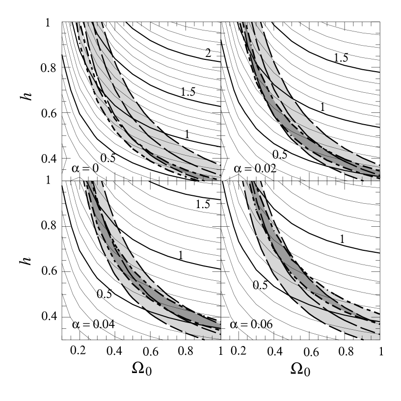
FIG. 2.: $\sigma_{8}(\alpha)$ as functions of $\Omega_{0}$ and $h$ normalized by COBE. The four panels correspond to $\alpha=0$ (top left), $0.02$ (top right), $0.04$ (bottom left) and $0.06$ (bottom right). The lightly shaded region inside the two short dash - long dash lines indicates the values of $\sigma_{8}$ observed from the X-ray clusters of the galaxies. The three long dashed lines represent shape parameters $\Gamma=0.2,0.25$ and $0.3$ from left to right, and the observationally favored region ($\Gamma=0.25\pm 0.05$) is also lightly shaded. The darkly shaded region satisfies the constraints from both the cluster abundances and the shape parameter.

FIG. 3.: The same as Fig. 2, except that the four panels correspond to $\alpha=0.08$ (top left), $0.10$ (top right), $0.12$ (bottom left) and $0.14$ (bottom right).

FIG. 4.: The power spectra for $\alpha=0.05,\Omega_{0}=0.4$ and $h=0.7$ (left panel) and $\alpha=0,\Omega_{0}=0.3$ and $h=0.7$ (right panel). The symbols denote the observational data. [5]

FIG. 5.: The solid lines represent values of $\alpha$ which give the best fit to the data of $\sigma_{8}$ from cluster abundances. The three long dashed lines represent shape parameters $\Gamma=0.2,0.25$ and $0.3$ from left to right.

FIG. 6.: Peak-height parameter $\gamma$ (see Eq.(11)) for $\alpha=0$ (top left), $0.04$ (top right), $0.08$ (bottom left) and $0.12$ (bottom right).

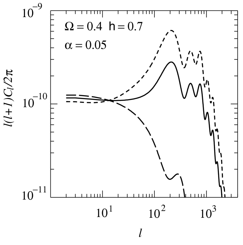
FIG. 7.: The CMB angular power spectra normalized by COBE. Here we have chosen $\Omega_{0}=0.4,\ h=0.7,\ \lambda_{0}=0.6$, and $\Omega_{B}h^{2}=0.015$. The short dashed line corresponds to the pure adiabatic case ($\alpha=0$), the long dashed line to the pure isocurvature case ($\alpha=\infty$), and the solid line to the case $\alpha=0.05$, which gives the best fit to the observational data.

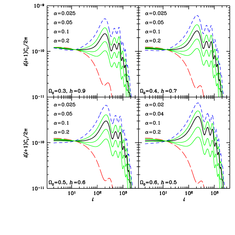
FIG. 8.: The same as Fig. 7, except that the cosmological parameters $\Omega_{0}$ and $h$ have been changed: $\Omega_{0}=0.3,\ h=0.9$ (top left), $\Omega_{0}=0.4,\ h=0.7$ (top right), $\Omega_{0}=0.5,\ h=0.6$ (bottom left) and $\Omega_{0}=0.6,\ h=0.5$ (bottom right). In this figure, we also plot angular power spectra for various $\alpha$ to see how much the acoustic peak decrease as $\alpha$ changes.

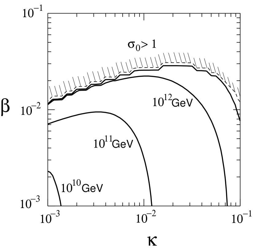
FIG. 9.: The Hubble parameter during the hybrid inflation, which is normalized by the COBE, ignoring tensor perturbations and isocurvature fluctuations. In the region above the dashed line, $\sigma_{0}$ exceeds the gravitational scale (i.e., $\sigma_{0}>1$) and it is excluded.

FIG. 10.: The Hubble parameter during the new inflation, which is normalized by the COBE, ignoring tensor perturbations and isocurvature fluctuations.

- [1] M. Kawasaki, N. Sugiyama, and T. Yanagida, Phys. Rev. D54, 2442 (1996).
- [2] R. Stomper, A. J. Banday and K. M. Górski, Astrophys. J. 463, 8 (1996).
- [3] S. D. Burns, astro-ph/9711303.
- [4] A. A. de Laix and R. J. Scherrer, Astrophys. J. 464, 539 (1996).
- [5] J. A. Peacock and S. J. Dodds, Mon. Not. Roy. Astron. Soc. 267, 1020 (1994).
- [6] T. Kanazawa, M. Kawasaki, N. Sugiyama and T. Yanagida, Prog. Theor. Phys. 100, 1055 (1998).
- [7] J.M. Bardeen, J.R. Bond, N. Kaiser and A.S. Szalay Astrophys. J. 304, 15 (1986).
- [8] N. Sugiyama, Astrophys. J. Supp. 100, 281 (1995).
- [9] M. Davis and P. J. E. Peebles, Astrophys. J. 267, 465 (1983).
- [10] C.L. Bennett et al., Astrophys. J. Letter 464, L1 (1996); E. Bunn and M. White, Astrophys. J. 480, 6 (1997).
- [11] H. Kodama and M. Sasaki Int. J. Mod. Phys. A1, 265 (1986); G. Efstathiou and J.R. Bond, Mon. Not. R. Astron. Soc. 227, 33 (1987); W. Hu and N. Sugiyama, Phys. Rev. D51, 2599 (1995).
- [12] V. R. Eke, S. Cole and C. S. Frenk, Mon. Not. Roy. Astron. Soc. 282, 263 (1996).
- [13] S. D. M. White, G. Efstathiou and C. S. Frenk, Mon. Not. Roy. Astron. Soc. 262, 1023 (1993).
- [14] P. T. P. Viana and A. R. Liddle, Mon. Not. Roy. Astron. Soc. 281, 323 (1996).
- [15] T. Kitayama and Y. Suto, Astrophys. J. 490, 557 (1997).
- [16] W.L. Freedman, astro-ph/9706072.
- [17] http://map.gsfc.nasa.gov/
- [18] http://astro.estec.esa.nl/SA-general/Projects/Planck/
- [19] V. F. Mukhanov, H. A. Feldman and R. H. Brandenberger, Phys. Rep. 215, 203 (1992).
- [20] H. Kodama and M. Sasaki, Int. J. Mod. Phys. A1, 265 (1986); A2, 491 (1987).
- [21] A. Linde and A. Riotto, Phys. Rev. D56, 1841 (1997).
- [22] J. Wess and J. Bagger, Supersymmetry and Supergravity (Princeton University Press, Princeton NJ, 1992).
- [23] E. J. Copeland et al., Phys. Rev. D49, 6410 (1994).
- [24] G. Dvali, Q. Shafi and R. Schaefer, Phys. Rev. Lett. 73, 1886 (1994).
- [25] S. Coleman and E. Weinberg, Phys. Rev. D7, 1888 (1973).
- [26] C. Panagiotakopoulos, Phys. Lett. B402, 257 (1997).
- [27] E. W. Kolb and M. S. Turner, The Early Universe (Addison-Wesley, Reading MA, 1990).
- [28] M. Kawasaki, T. Moroi and T. Yanagida, Phys. Lett. B383, 313 (1996).
- [29] Izawa K-. I. and T. Yanagida, Phys. Lett. B393, 331 (1997).
- [30] K. Kumekawa, T. Moroi and T. Yanagida, Prog. Theor. Phys. 92, 437 (1994).
- [31] A. D. Linde, Phys. Lett. B259, 38 (1991).
- [32] A. G. Riess et al., astro-ph/9805201.
- [33] T. Banks and M. Dine, Nucl. Phys. B479, 173 (1996); Nucl. Phys. B505, 445 (1997).
- [34] M. Kawasaki and T. Yanagida, Prog. Theor. Phys. 97, 809 (1997).