AGAPEROS: Searches for microlensing in the LMC with the Pixel Method

Abstract

We apply the pixel method of analysis (sometimes called “pixel lensing”) to a small subset of the EROS-1 microlensing observations of the bar of the Large Magellanic Cloud (LMC). The pixel method is designed to find microlensing events of unresolved source stars and had heretofore been applied only to M31 where essentially all sources are unresolved. With our analysis optimised for the detection of long-duration microlensing events due to 0.01-1 $M_{\odot}$ Machos, we detect no microlensing events and compute the corresponding detection efficiencies. We show that the pixel method, applied to crowded fields, should detect 10 to 20 times more microlensing events for $M>0.05M_{\odot}$ Machos compared to a classical analysis of the same data which latter monitors only resolved stars. In particular, we show that for a full halo of Machos in the mass range 0.1 – 0.5 $M_{\odot}$, a pixel analysis of the three-year EROS-1 data set covering $0.39\,\rm deg^{2}$ would yield $\simeq 4$ events.

1 Introduction

Microlensing searches can probe the distribution of MAssive Compact Halo Objects (Machos) in the dark halo of our Galaxy or more distant galaxies (Paczyński (1986,1996), Griest (1991)). Several lines of sight are now under investigation, and events have been claimed in several directions: towards the LMC (Alcock et al. 1997a, Renault et al. 1997), the SMC (Alcock et al. 1997b, Palanque-Delabrouille et al. 1998), in the direction of the Galactic Bulge (Alard et al. 1997, Alcock et al. 1997c, Udalski et al 1994) and more recently towards spiral arms (Derue et al. 1998), giving some first evidences of the Macho distribution towards these lines of sight. These results are based on a star monitoring analysis: the fluxes of several millions of resolved stars are monitored. As first discussed by Crotts (1992) and Baillon et al. (1993), events due to unresolved stars essentially escape detection of these analyses. Such stars, beyond the crowding limit or too dim to resolve, could significantly contribute to the number of detectable events. This is illustrated by the detection of two variable objects in the MACHO analysis (Alcock et al. 1997a) of LMC data, which could not be resolved at their minimum luminosity. The detection of the variation was nevertheless possible because the reference images used to establish the catalogue of monitored stars were taken during their maximum luminosity, when the stars were resolved. However, such events can neither be kept for further considerations nor be included in the computation of detection efficiencies, in the star monitoring approach.

In this paper, we apply a pixel analysis to the EROS 91-92 data (10% of the whole EROS-1 CCD data set) of the LMC Bar. The idea is to monitor the flux of all the pixels present on the images, thus achieving a good sensitivity to the whole stellar content of the images. The magnification of one unresolved star can be detected as a variation of the pixel flux, provided that the magnification is high enough. – In the following, we will refer to this approach as pixel monitoring, as opposed to star monitoring referring to classical analyses restricted to resolved stars. – The main uncertainties of this approach concern our ability to account properly for variations of the observational conditions, and to be able to disentangle intrinsic variations from observational systematics. In Paper I (Melchior et al. 1998a), dedicated to the description of the treatment of the data and the production of $2.1\times 10^{6}$ super-pixel light curves, we have shown that an average stability of $1.8\%$ of the super-pixel flux is achieved in blue and $1.3\%$ in red, about twice the expected photon noise. This homogeneous set of super-pixel light curves is called AGAPEROS: each of these light curves covers a period of $120$ days and is composed of about 90 measurements. With this rather short period of observation, we show here how it is possible to investigate the Macho mass range of interest ($M\simeq 10^{-2}-1M_{\odot}$) with the existing EROS-1 CCD data set, initially designed for short time scale events in a mass range ($M\simeq 10^{-8}-10^{-3}M_{\odot}$) where no event has been detected.

Microlensing selection with the Pixel Method

We first present the simple formalism used to describe the pixel events in which we are interested. The pixel flux $\phi^{p}$, affected by a microlensing event, can be written as:

$$\phi^{p}_{i}=\alpha_{i}A(t_{i})\phi^{*}_{i}+\phi^{\rm bg}_{i}$$ (1)

where $i$ is the measurement number, $t$ is the time, $\alpha$ is the seeing fraction, $A$ the magnification, $\phi^{*}$ the flux of the star of interest at rest (i.e., unmagnified), and $\phi^{\rm bg}$ includes the sky and stellar backgrounds. The magnification (Paczyński 1986) depends on the normalized impact parameter $u(t_{i})$:

$$A(t_{i})=\frac{u^{2}+2}{u\sqrt{u^{2}+4}}$$ (2)

with

$$u(t_{i})=\sqrt{u_{0}^{2}+{\left(\frac{v_{T}}{R_{E}}\right)}^{2}(t_{i}-t_{0})^{2}}$$

where $v_{T}$ is the Macho transverse velocity, $u_{0}$ and $t_{0}$ the impact parameter and time of closest approach, and $R_{E}$ the Einstein radius:

$$R_{E}=\sqrt{\frac{4GM}{c^{2}}\frac{D_{OL}D_{LS}}{D_{OS}}}$$

The typical time scale of the variation is the Einstein radius crossing time:

$$t_{E}=\frac{R_{E}}{v_{T}}$$ (3)

In Paper I, we showed that the variations of the observational conditions, which obviously affect Eq. 1, can be corrected: each image is first geometrically aligned with the reference image. Then sky background and absorption factor are corrected to the values of the reference image. Finally, each super-pixel flux is adjusted to take account of the seeing variation, affecting $\alpha_{i}$. Since the mean seeing is about $3$ arc-second, we estimate $\alpha$ to be on average $0.7$ for the corrected $3.\hskip-2.0pt^{\prime\prime}6\times 3.\hskip-2.0pt^{\prime\prime}6$ super-pixel light curves, obtained in Paper I. We showed that in the absence of microlensing events ($A\left(t_{i}\right)=1$), we achieve a proper understanding of the errors affecting these light curves, and that Eq. 1 describes to a good approximation the light curves we are studying.

The usual requirements used for the selection of microlensing events detected by star monitoring can be applied here:

• As the microlensing phenomenon is a transient and rare phenomenon, it should produce a unique significant variation in the star flux.

• It must be achromatic. This characteristic has two applications for a pixel analysis: the time of the maximum has to be the same in both colours and the ratio

  $$\frac{{{\phi^{p}_{i}}^{(B)}}-\phi^{(B)}_{\rm bg}}{{\phi^{p}_{i}}^{(R)}-\phi^{(R)}_{\rm bg}}$$ (4)

  must remain constant, during the variation.

• The shape must be compatible with Eq. 1.

The first criterion allows us to remove recurrent variable stars as well as most of the noise, while the two other criteria will be applied to the few remaining light curves at the end of the selection process.

• Last, we consider the fact that the probability for a star to be lensed is independent of its type. This will allow us to reject specific populations of variable stars.

In Sect. 2, we present the Monte-Carlo simulations used in this article. Then, in Sect. 3, we describe step by step the selection procedure designed to detect microlensing events and applied to these light curves. In Sect. 4, we show how the selected variations can be eliminated as compatible with variable stars. In Sect. 5, we discuss the detection efficiencies achieved by this analysis, and compare the number of expected events with the sensitivity of star monitoring. We rely on these results in Sect. 6 to discuss the possible prospects of this approach.

2 A useful tool: mock super-pixel light curves with microlensing events

Monte-Carlo simulations described in Baillon et al. (1993) gave a first estimate of the number of events expected with a pixel analysis. The main uncertainties discussed there derived from the noise present in real data. In Sect. 2.1, we present a summary of the simulations of microlensing events used in this paper. These model the physical ingredients including the halo density profile, the luminosity function of source stars, and the Macho velocity distribution and mass function (see Baillon et al. 1993). In Sect. 2.2, we define a minimal threshold that will be useful later on for the interpretation of the results of our analysis. In Sect. 2.3, we discuss the characteristics of the simulated events as expected for an ideal analysis of our data set. Last, in Sect. 2.4, we add to this model the characteristics of the AGAPEROS data, and thus produce realistic mock super-pixel light curves. This tool will be used in the following to adjust the selection criteria in Sect. 3 and to compute the detection efficiencies in Sect. 5.

2.1 Physical ingredients

We assume an isothermal halo with a core radius of $5$ kpc, normalized at the solar neighbourhood to $\rho_{\odot}=8.\times 10^{-3}{M_{\odot}}pc^{-3}$ (Flores 1988) and filled with compact objects with a given mass $M$ as discussed by Griest (1991). We adopt a LMC distance of $50$ kpc. The corresponding optical depth for a full halo is the same as the one used by the MACHO group (Alcock et al. 1997a) $\tau_{full}\leavevmode\nobreak\ =\leavevmode\nobreak\ 4.7\leavevmode\nobreak\ \times 10^{-7}$. It is to be noted that our estimate of the expected number of events assumes a full halo and it should be multiplied by a factor $f<0.5$ according to the MACHO and EROS results (Alcock et al. 1997a, Renault et al. 1997), where $f$ is the halo fraction actually filled with Machos. According to the MACHO results (Alcock et al. 1997a), it is most probably smaller than $0.5$. Note that no halo flattening has been considered at this stage, but more sophisticated models could be implemented and tested once serious candidates are detected.

We calculate the number of potential lenses with a fixed mass $M$ located in the cone pointing towards our field of view. We assign a random position to the Macho and choose its transverse velocity $v_{T}$ from a two-dimensioned Maxwellian distribution $g(v_{T})$ weighted by $v_{T}$. For each given Macho, we determine the probability that a star will lie close enough to this line of sight to give rise to a microlensing event. We use the luminosity function described in Baillon et al. (1993) which is based on Hardy et al. (1984) for the bright stars, on Ardeberg et al. (1985) up to magnitude $V=23$ and is extrapolated to the faint end using the luminosity function of the solar neighbourhood (Allen 1973). Note that on the one hand, the details of this latter extrapolation are not important because, as we show below, few events are detectable for sources fainter than $V=24$; but on the other hand, the connection between these 3 sets of observations is a source of uncertainties.

Figure 1: Luminosity function used for the simulations: the number of stars per arcsec² or per pixel ($1.\hskip-2.0pt^{\prime\prime}21\times 1.\hskip-2.0pt^{\prime\prime}21$), normalised to a surface brightness $\mu_{V}=21$ is exhibited as a function of the V magnitude. This shows the typical stellar content of a pixel.

This luminosity function is displayed in Fig. 1 and is quite compatible with recent measurements (Holtzman et al. 1997, Ardeberg et al. 1997). We then normalize this function to a surface brightness of $\mu_{V}=21$ (de Vaucouleurs 1957). The star’s magnitude is drawn from a uniform distribution and the simulated event is then weighted according to the luminosity function. As described in Baillon et al. (1993), we account for possible finite source effects that are expected when the stellar radius projected onto the plane of the Macho is comparable with the Einstein radius. We are then able to compute the number of expected events using well-known Monte-Carlo integration techniques.

2.2 Minimal requirements for simulated microlensing events

We require here some minimal requirements that will define a set of simulated microlensing events that could be detected with an ideal experiment.

As we do not expect to detect a significant number of low-magnification events, we introduce a threshold $A_{max}>1.34$ in our simulations. Detectable low-magnification events affect bright stars and hence would have already been detected by the previous EROS star monitoring analysis anyway. Moreover, the magnification by such a small factor of a dim star would be completely buried into the noise, therefore one must add a visibility condition. We choose the following: at the time of maximum magnification, the flux of the central super-pixel of a magnified star should rise higher than $3\sigma$ above the background, $\sigma$ being taken as twice the photon noise. It is important to note that this threshold does not depend on the duration of the event. It only removes events that we would not detect in any case.

The effect of this requirement on the characteristics of the simulated sample can be seen in Fig. 2. The impact parameter distribution is no longer expected flat. This $3\sigma$ threshold introduces a (necessary) bias into the impact parameter distribution towards small values. The majority of the events are expected to affect dim stars with a small impact parameter $u_{0}<0.2$.

The simulations including these two thresholds ($A>1.34$, and S/N $>3\sigma$) will be used as a reference for the computation of our detection efficiency in Sect. 5.

Figure 2: Initial set of the simulated light curves with some microlensing events. The distributions of the impact parameters $u_{0}$ (panel a) and of the $V$ magnitude of the un-magnified star (panel b) are exhibited. The histograms shown are computed for 0.5 $M_{\odot}$ Machos. At this stage simulations with different Macho’s mass will give the same histograms but with a different normalization.

2.3 Preliminary estimates

Firstly, we discuss the number of microlensing that can be expected with an ideal experiment. Secondly, we estimate the number of stars effectively monitored in our reference set.

2.3.1 Number of expected events

The number of microlensing events estimated by our simulations for a halo filled with Machos of mass $M$ is thus defined as:

$$N_{\rm evt}=\int d\phi^{*}\Biggl{[}N_{\rm stars}(\phi^{*})\times T_{\rm obs}\int dv_{T}\biggl{[}v_{T}g(v_{T})\times$$

$$\int dD\Bigl{[}2u_{0}(\phi^{*})R_{E}(D)\frac{f\ \rho(D)}{M}\times\epsilon(\phi^{*},t_{E}(M,D,v_{T}))\Bigr{]}\biggr{]}\Biggr{]}$$ (5)

where $N_{\rm stars}(\phi^{*})$ is the true number of stars with a flux between $\phi^{*}$ and $\phi^{*}+d\phi^{*}$ present in the sky area studied, $T_{\rm obs}$ is the duration of the observations (120 days), $\rho(D)$ the Macho density distribution, $D$ the position of the Macho and $\epsilon$ is the efficiency ($\epsilon=1$ for an ideal experiment).

Table 1: Number of expected microlensing events as a function of the Macho mass, given the minimal requirements discussed in the text.

$M/M_{\odot}$	$0.01$	$0.05$	$0.1$	$0.5$	$1.0$
$N^{\rm AGAPEROS}_{\rm evt}/f$	$9.8$	$4.4$	$3.1$	$1.4$	$1.0$

Tab. 1 gives the number of microlensing events that can be expected with an ideal analysis of the super-pixel light curves produced in Paper I. In the large-mass range, where all the known microlensing candidates on the LMC have been identified, we expect between 1 and 10 microlensing events assuming a full halo.

2.3.2 Effective number of monitored stars

If we were able to select all light curves of our reference sample, we would define the equivalent number of monitored stars $N^{\rm AGAPEROS}_{\rm stars}$ as follows:

$$N_{\rm stars}^{\rm AGAPEROS}\equiv\int d\phi^{*}N_{\rm stars}(\phi^{*})u_{0}(\phi^{*}|3\sigma)$$ (6)

$u_{0}(\phi^{*}|3\sigma)$ is the threshold impact parameter that enters Eq. 5 which accounts for the $3\sigma$ deviation imposed at the time of maximum magnification in Sect. 2.2. Actually, this number $N^{\rm AGAPEROS}_{\rm stars}$ would only depend on the luminosity function and the definition of our reference sample. Hence, we can consider that we effectively monitor the equivalent of $2.2\times 10^{6}$ stars, whose mean magnitude is $22.1$ (see Fig. 2b).

If one integrates the luminosity function (Fig. 1) over a pixel area ($1.\hskip-2.0pt^{\prime\prime}21\times 1.\hskip-2.0pt^{\prime\prime}21$), one finds one star in the magnitude range $20-24$, that could undergo a microlensing event. This explains why the effective number of stars thus defined is of the same order as the number of pixels.

2.4 Model of the data

The idea is to simulate super-pixel light curves that include microlensing events. We compute the flux of the star – affected by a microlensing variation – which enters the $3.\hskip-2.0pt^{\prime\prime}6\times 3.\hskip-2.0pt^{\prime\prime}6$ super-pixel. We also add a background flux – together with expected read-out and photon noises – in order to obtain realistic mock light curves. The computation of these fluxes takes account of the pass-band of the filters, the quantum efficiency of the CCD camera and its gain. (See Paper I and references therein for more quantitative information about the characteristics of the raw data.) Actual spacing and variations of the observational conditions (absorption and sky background), measured on the data, are also taken into account in this procedure. Similarly to what is done for real data, the averaging procedure of the measurements available each night is applied to these mock light curves, as well as to the computation of error bars. We multiply these errors, assumed to be gaussian and uncorrelated, by the factor found in Paper I between the measured dispersion and the expected photon noise.

We finally get mock light curves typical of the microlensing events we are looking for. Fig. 3 displays two examples of typical expected events.

Figure 3: Two examples of simulated super-pixel light curves containing a microlensing event.

3 Selection of microlensing events

We apply a pixel analysis designed to select microlensing events on the EROS 91-92 data of the LMC. Using the methods described in Paper I and applied on the AGAPEROS data set, we constructed some $2.1\times 10^{6}$ (real) super-pixel light curves, cleaned of all observational effects and corrected for systematic effects to the degree possible. In this section, we define a selection process designed to select possible microlensing events. The application of a basic trigger – detection of bumps – reveals a large number of variations, most of them corresponding to obvious variable stars, but also to some noisy variations that we will have to eliminate. Owing to the averaging of the images taken each night (see Paper I), some of the variations are most probably due to short-time scale variables already studied elsewhere (Beaulieu 1995, Grison 1995). As Renault et al. (1997,1998) have already excluded the small-mass Macho range with this data set, we choose to optimise our sensitivity to long time-scale variations, corresponding to the large-mass range in which all the known microlensing events have been detected.

The selection criteria should remove intrinsic variations and systematic effects, keeping genuine microlensing events. We describe these various criteria successively applied to the data. Some rather loose cuts, applied on super-pixel light curves, turn out to be sufficient to reduce considerably the number of light curves to analyse. Then a visual inspection of the 120 remaining curves confirms that they are affected by genuine variations and they will be further studied in Sect. 4. The efficiency of our selection procedure with simulated super-pixel light curves has been checked in both colours.

We work on a simulation based on $5\times 10^{6}$ realizations, which allows to have small statistical errors on the number of expected events. The number of events given at each step of the selection procedure is calculated assuming a halo full of $0.5M_{\odot}$ Machos. In Sect. 5, we discuss the sensitivity actually achieved in a larger-mass range $0.01M_{\odot}\leq M\leq 1M_{\odot}$.

The selection procedure, defined in this section and summarised in Tab. 2, splits into $3$ steps: (1) a significant variation must be present in at least one colour. (2) Light curves with any significant secondary variations are eliminated. (3) A correlation between the two colours is required. The two first thresholds are based on the following definition of the variations or “bumps”.

Table 2: Summary of the selection procedure: the percentage of events kept at each steps is given for the simulations (2nd column) and the data (4rd column). The 3rd and 5th columns give the number of simulated and real light curves kept.

	Simulations		Data
Starting from	$1.4$		$2.1\times 10^{6}$
	events		light curves
One bump
- $L_{1}>500$	51.0%	0.71	0.25%	5 338
- 3 points above 3$\sigma$	71.2%	0.51	52.3%	2 789
No second bump	90.3%	0.46	77.5%	2 162
Good correlation	85.5%	0.39	5.5%	120

Definition of a bump

A baseline $\phi_{bl}$ is calculated for each super-pixel light curve as the minimum of a running average over 5 successive flux measurements. $\sigma_{bl}$ is the error associated with the baseline flux determination. All the light curves are scanned for the detection of bumps, defined as at least $3$ consecutive measurements lying above the baseline by at least $3\sigma_{n}$

$$\sigma_{n}=\sqrt{{\sigma^{\prime}_{n}}^{2}+{\sigma_{bl}}^{2}}$$ (7)

where ${{\sigma}^{\prime}_{n}}$ is the error associated to each super-pixel flux computed in paper I for the night $n$. The bump ends when at least 2 consecutive measurements lie below this threshold. Each bump $i$ is characterised using a likelihood function:

$$L_{\mathrm{i}}=-\ln\left(\prod_{n\in\mathrm{bump\leavevmode\nobreak\ i}}P(\phi\geq\phi_{n})\ \mbox{ given }\ \left\{\begin{array}[]{c}\phi_{bl}\\ \sigma_{n}\end{array}\right.\right)$$ (8)

$\phi_{n}$ is the super-pixel flux for the measurement $n$, whose computation for all the light curves is detailed in Paper I.

3.1 At least one significant variation

Firstly, we require one significant bump in at least one colour. Secondly, we then look for a minimal variation in the other colour.

A large bump in at least one colour

In order to identify significant variations, we require the likelihood function $L_{1}$ associated with the largest fluctuation to be larger than $500$ for at least one colour. This value is chosen using the Monte-Carlo simulations to optimise the S/N ratio. In a given colour, we search for clusters of super-pixels having each $L_{1}$ larger than 500. We then select the central super-pixel of each cluster, if it also satisfies the $L_{1}>500$ requirement. The latter requirement is intended to remove some artifacts, in particular close to bright stars. The next cuts will be applied on these central super-pixels.

Minimal variation in the other colour

The previous cut has allowed to detect significant variations in at least one colour. We now require that the first fluctuation of the central super-pixels of the other colour to have at least $3$ consecutive points $3\sigma$ above the baseline. Although it corresponds to a quite small value of $L$ ($\simeq 15$), it constitutes a first requirement of achromaticity.

3.2 No significant second bump

Figure 4: Super-pixel light curve with several variations rejected with the cut on $L_{2}$ ($L^{B}_{1}=1366.$ ; $L^{R}_{1}=2958.$ ; $L^{B}_{2}=565.$ ; $L^{R}_{2}=1655.$). The upper curve exhibits the light curve in blue and the lower one in red.

At this stage, we have selected super-pixel light curves with at least one significant variation. Now, it is important to check uniqueness. We then require the second most significant fluctuation to have $L_{2}<250$ in both colour. Fig. 4 shows an example of rejected light curves with two variations.

3.3 Correlation between the two colours

Figure 5: Histogram of the correlation factor computed between the two colours. The hatched area corresponds to super-pixel light curves with a correlation factor below the threshold $\rho=0.8$. The histogram superimposed with a dashed line on this figure corresponds to the simulations and scales with the tick marks and values given on the right axis.

Figure 6: Super-pixel light curve with a shape compatible with a microlensing event. ($L^{B}_{1}=641.$ ; $L^{R}_{1}=744.$ ; $L^{B}_{2}=57.$ ; $L^{R}_{2}=0.$ ; $\rho=0.84$)

Figure 7: Super-pixel light curve with a shape incompatible with a microlensing event ($L^{B}_{1}=1386.$ ; $L^{R}_{1}=16416.$ ; $L^{B}_{2}=80.$ ; $L^{R}_{2}=0.$ $\rho=0.93$)

Figure 8: Super-pixel light curve for which it is inconclusive. ($L^{B}_{1}=1791.$ ; $L^{R}_{1}=12927.$ ; $L^{B}_{2}=0.$ ; $L^{R}_{2}=176.$ $\rho=0.96$)

In order to select the expected long time-scale variations, we choose for the next requirement a reasonable correlation between the blue and red light curves.

Given the constraints mentioned above, the correlation $\rho^{p}_{\rm col}$ between the two colours:

$$\rho^{p}_{\rm col}=\frac{\sum_{n}{\left(\phi^{p}_{n}-{\langle\phi\rangle}\right)}_{\rm blue}{\left(\phi^{p}_{n}-{\langle\phi\rangle}\right)}_{\rm red}}{\sqrt{{\sum_{n}{\left(\phi^{p}_{n}-{\langle\phi\rangle}\right)}^{2}}_{\rm blue}\sum_{n}{{\left(\phi^{p}_{n}-{\langle\phi\rangle}\right)}^{2}}_{\rm red}}}$$ (9)

achieves a good sensitivity to the achromaticity and to the dispersion of the measurements. As shown by the mock light curves in Fig. 5 (dashed curve), a clear correlation between the two colours is expected: most of the mock curves (85.5%) lie above a threshold $\rho=0.8$. Fig. 5 displays the corresponding histogram for the real light curves selected so far (full line). This distribution is quite different and exhibits a peak close to $\rho=0$. With a threshold at $\rho^{p}_{col}>0.8$, 94.4% of the remaining light curves are removed: $120$ variations remain. Fig. 6 displays one of these light curves: its shape is in quite good agreement with what we can expect from a microlensing event although the period of observation is short compared to the duration of the variation, and it is not possible to test up to now the uniqueness of the variation. Fig. 7 displays another light curve, one whose shape is clearly incompatible with a standard microlensing event. Fig. 8 shows a light curve for which it is impossible to draw any conclusion based only on compatibility with the microlensing shape: the period of observation is much shorter than the time-scale of the variation.

When the criteria described above are applied in the simulations, we expect $0.38\times f$ events for $0.5M_{\odot}$ Machos filling a fraction $f$ of the halo. It is obvious then that the $120$ selected light curves are in clear excess with respect to what is expected and need to be further studied.

4 Colour magnitude diagram

Figure 9: Colour magnitude diagram: the small dots corresponds to the stars detected by the EROS-1 star monitoring analysis (Renault, 1996). The circles corresponds to the 120 selected variations discussed in the text. Among them the filled circles are Miras detected by Hughes (1989) in the I band (see text).

Since the expected background for microlensing events is due to variable stars, we have first to determine the position of the $120$ light curves with variations on the colour magnitude diagram (CMD), before drawing any conclusion on the nature of these variations. The problem is now to know how we can estimate the magnitude of the underlying star responsible for the observed variation.

4.1 Magnitude determination

Using an image with a seeing close to the mean value ($3$ arc-second) – for which no significant seeing correction is required – we perform photometry on the surrounding stars using DAOPHOT which returns the total background lying within $2$ arc-second of the center of the super-pixel. We then subtract this background from the super-pixel flux measured when the star is at maximum luminosity, and account for the seeing fraction of the star flux entering the super-pixel. Hence, we deduce the magnitude of the star at the maximum. Due to the crowding of the LMC Bar, this aperture photometry is the most efficient way to estimate a magnitude for the stars responsible of the detected variations. More details about magnitude determination will be further addressed in Melchior et al. (1998b).

This estimate is mainly intended to study the position in the CMD of the dominant source of flux of the varying pixel and in particular if it lies in marginal locations of the colour-magnitude diagram, characteristic of variable stars. We estimate the uncertainties on this magnitude determination as the square root of the sum of the squares of the two following components. The first is the error on the super-pixel flux. The second one is estimated as 10% of the “star” flux and is expected due to uncertainties in the star position inside the inner pixel of the super-pixel. In extreme cases – when the star flux at maximum is not the main contribution of the super-pixel flux – these errors can be underestimated.

4.2 Discussion

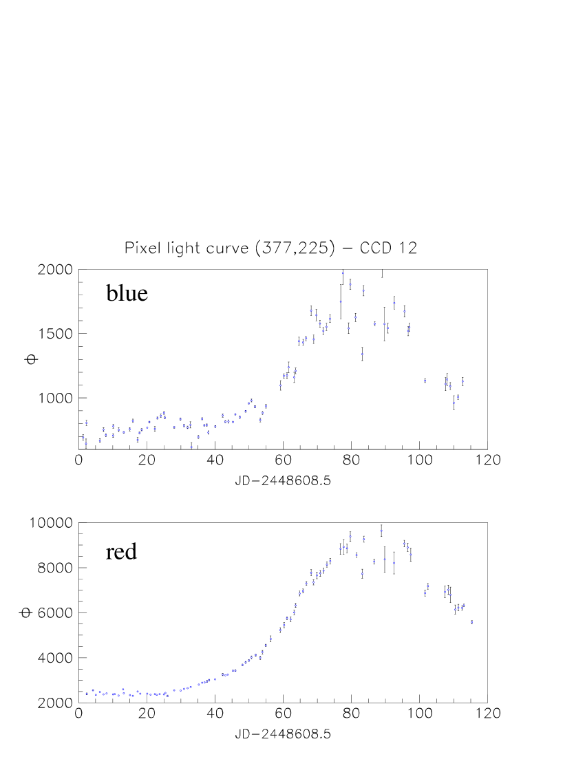
Figure 10: Super-pixel light curve with a variation detected by our analysis which has been identify as a Mira. ($L^{B}_{1}=10188.$ ; $L^{R}_{1}=47940.$ ; $L^{B}_{2}=112.$ ; $L^{R}_{2}=0.$ $\rho=0.96$)

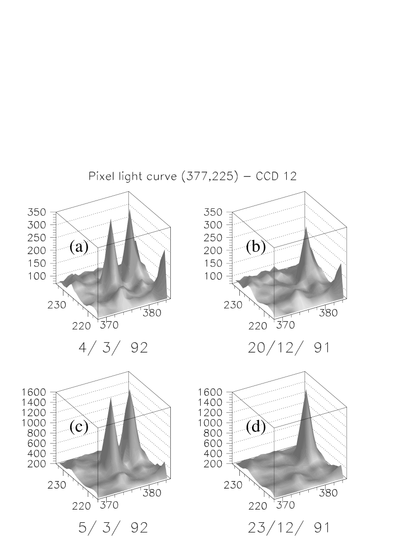
Figure 11: Map of the surroundings of the Mira whose light curve is displayed on Fig. 10: each figure displays the flux as a function of position on an area of $20.6\arcsec\times 20.6\arcsec$. Upper figures a and b correspond to blue images, and lower ones c and d to red images. Figures a and c on the left side exhibit the star at the maximum of the variations. On the figures on the right side b and d, this star has disappeared in the background. Note that such an event would have escaped any star monitoring, and could not have been accounted for as part of a blend.

Table 3: Miras: matches with a previous study by Hughes (1989). The following characteristics are given: the position at 1950.0 epoch, the CCD number, the pixel position, the mean $I$ magnitude, the period in days

$\alpha$ $\delta^{a}$	CCDb	ix iyb	$I^{a}$	Perioda
5.:16.:50.9 -69.:37.:52.0	0	295 220${}^{\leavevmode\nobreak\ }$	13.87	170
5.:16.:57.0 -69.:19.: 9.0	8	93 545${}^{\leavevmode\nobreak\ }$	14.36	183
5.:18.:19.7 -69.:41.:30.0	1	301 125${}^{\leavevmode\nobreak\ }$	14.04	296
5.:20.:15.8 -69.:30.:59.0	10	252 173${}^{\leavevmode\nobreak\ }$	14.96	293
5.:20.:35.5 -69.:43.:22.0	3	59 180c	13.21	650
5.:21.: 8.7 -69.:37.:37.0	3	135 493d	13.11	453
5.:21.:43.1 -69.:43.:28.0	3	346 240${}^{\leavevmode\nobreak\ }$	13.94	453
5.:21.:47.6 -69.:43.:12.0	3	361 258${}^{\leavevmode\nobreak\ }$	14.90	210
5.:23.:13.6 -69.:38.:45.0	4	258 556${}^{\leavevmode\nobreak\ }$	13.77	255
5.:23.:52.9 -69.:34.:12.0	12	377 225e	14.40	163

^aSource: Hughes (1989) ^bSource: AGAPEROS, this analysis ^cCf. Fig. 7 ^dCf. Fig. 8 ^eCf. Figs. 10 and 11

Fig. 9 displays a CMD with the stars detected by the EROS group (dots) and the underlying stars (circles) associated with the selected super-pixel light curves. The variations kept by our analysis are not representative of the bulk of the stars: all of them but two lie in the red part of the CMD.

The 118 red variable stars

The red detected variable stars are all located in the same area of the colour magnitude diagram. We have even been able to check that $10$ of them have already been recorded by Hughes (1989) as Miras with a study in the I band. They are displayed with filled circles on Fig 9 and their known characteristics are displayed in Tab. 3. Fig. 10 exhibits the light curve of one of these Miras, with a $163$ days period. Not surprisingly the variation is significant but only sampled over $120$ days, and this is the shortest period of the Miras listed in Tab. 3. Two of these Miras have been shown previously. One is presented in Fig. 7, it has a period of $650$ days. Another one is exhibited in Fig 8 with a period of $453$ days. The catalogue of Hughes (1989) contains $41$ variable stars overlapping the field studied here and most of them have been rejected at an earlier stage of this analysis. The thick lines show the area of the CMD excluded by the EROS group corresponding to the regions where variable stars are expected. It is then highly probable that the other red variable stars selected are also Long Period Variables, as they lie in the same area of the CMD. The fact that the majority of the red variable stars selected by this analysis have not been identified previously demonstrates the potential interest of the pixel method for the detection of Long Period Variable (LPV) stars with respect to classical analysis restricted to the study of resolved stars. A comprehensive analysis of these variable stars rejected as background of the microlensing search will be presented elsewhere (Melchior et al. 1998b).

About 10 of these red variable stars lie below the crowding limit and Fig. 10 displays the light curve of one of them: the Mira already discussed above. For these stars, we are not able to detect variations around their minimum flux. This is illustrated in Fig. 11 which shows the field surrounding this star: an unresolved star has exhibited a variation. Although this particular example would have escaped the EROS-1 star monitoring applied on the same data, it has already been identified in another wavelength (I band) by Hughes (1989).

The 2 blue variable stars

Figure 12: Super-pixel light curve with a variation affecting a blue star detected by our analysis. It has been detected previously by Beaulieu et al. (1996) and identified as a pre-main-sequence star candidate labelled ELHC2. ($L^{B}_{1}=1747.$ ; $L^{R}_{1}=3850.$ ; $L^{B}_{2}=0.$ ; $L^{R}_{2}=146.$ $\rho=0.89$)

The brightest blue variable star (with $B_{E}\simeq 15$) shown in Fig. 12 belongs to the sample of pre-main-sequence stars selected by Beaulieu et al. (1996). The short time scale variation which superimposes on long-time scale 0.3 magnitude variation is real and this feature excludes the simple microlensing interpretation anyway.

The other blue variable star is characterised by a small amplitude ($\Delta B_{E}<0.3$) and a duration longer than $120$ days. These features together with the position of this variable in the CMD indicate that the variation is compatible with the new class of variable stars called the blue bumpers identified by the MACHO group (Cook et al. 1995, Alcock et al. 1996).

4.3 Final cut on the colour magnitude diagram

These considerations provide convincing evidences that the selected variations are variable stars (Long Period Variables for most of them). We decide to apply the same cut as EROS on the CMD, displayed with the thick lines shown in Fig. 9. These regions are filled with a negligible number of stars ($<$ 1.3%), that are moreover expected to be variable. The elimination of this area does not significantly affect our sensitivity to microlensing events which are expected to occur independently of the star’s position in the colour-magnitude diagram.

5 Results

Table 4: Percentage of events kept for each step of the selection procedure for different Macho’s mass. The last row provides the percentage of events kept with respect to the initial set of events.

$M/M_{\odot}$	$0.01$	$0.05$	$0.1$	${\mathbf{0}.5}$	$\mathbf{1}$
$L_{1}>500$ in at	32.0%	42.1%	43.7%	48.9%	48.4%
least one colour
3 pts above 3$\sigma$	44.1%	58.6%	65.0%	71.2%	72.9%
in both colours
$L_{2}<250$ in	96.4%	93.3%	92.9%	89.7%	89.4%
both colours
$\rho>0.8$	75.9%	76.0%	75.0%	85.5%	88.7%
Total efficiency	10.3%	17.4%	19.8%	26.7%	27.9%

Although we detect no microlensing events with the selection procedure described above, we would have detected them if there were some. Whereas the detection of variable stars gives a first idea of the sensitivity achieved by this analysis, the Monte-Carlo simulations provide detection efficiencies. Firstly, we present the detection efficiencies achieved for this pixel analysis. Secondly, we compare our sensitivity with those achieved by star monitoring analyses.

5.1 Detection efficiencies for pixel monitoring

Figure 13: Detection efficiencies computed as a function of the Einstein radius crossing time ${t_{E}}$.

In Sect. 3, we detail the effect of the selection procedure on simulated light curves. For the clarity of the discussion, we restricted then the comparison to events expected with a halo full of $0.5M_{\odot}$ Macho. We study here the sensitivity achieved by our selection procedure on a larger-mass range. Tab. 4 shows the percentage of simulated events selected by each step of our selection procedure for $0.01M_{\odot}\leq M\leq 1M_{\odot}$. It appears clearly that we have optimised the selection procedure for this Macho mass range, and that efficiency is lost with decreasing Macho mass. The last cut on the correlation factor ($\rho>0.8$) is less favourable for $M\leq 0.1M_{\odot}$: for variations affecting only part of the period of observation, it is more optimal to restrict the computation of this coefficient to the portions of the light curve undergoing variations.

Figure 14: Selected simulated light curves. The distributions of the impact parameter $u_{0}$ (a) and of the $V$ magnitude (b) of the star at rest are exhibited, for 0.5 $M_{\odot}$ Machos. Normalisation corresponds to a full halo.

Figure 15: Selected simulated light curves. The distributions of the impact parameter $u_{0}$ (a) and of the $V$ magnitude (b) of the star at rest are exhibited, for 0.01 $M_{\odot}$ Machos. Normalisation corresponds to a full halo.

These efficiencies can be studied as a function of the duration ${t_{E}}$ as shown in Fig. 13. Due to the temporal sampling, the selection procedure is less efficient for short duration events. The efficiency remains constant for long-duration events, as we do not require a stable baseline.

Fig. 14 shows the distribution of impact parameters and V magnitude for simulated events due to 0.5 $M_{\odot}$ Machos satisfying all our requirements. It is clear that with respect to Fig. 2, the selection procedure eliminates microlensing events affecting very dim stars ($V>24$), and that the main contribution is expected due to events affecting dim stars with a small impact parameter. Fig. 15 gives the same histograms but for events due to $0.01M_{\odot}$ Machos. Events affecting dim stars are much more difficult to detect if they are short. Hence, detected events affect on average brighter stars and the impact parameter distribution appears flatter.

Figure 16: Detection efficiencies computed as a function of the magnitude of the un-magnified star.

Fig. 16 exhibits the detection efficiencies achieved as a function of the V magnitude of the un-magnified star and illustrates the previous point. The longer the events, the dimmer the stars they can affect. It is also to be noted that events affecting bright stars can be missed when the event duration is longer than the period of observation.

5.2 Comparison with star monitoring

Table 5: Number of expected microlensing events for this pixel analysis and the EROS star monitoring analysis. The 2nd row gives the number of events $N^{\rm AGAPEROS}_{\rm evt}$ expected given these efficiencies and a halo mass fraction $f$, that can be compared with the number of events $N^{\rm EROS}_{\rm evt}/f$ expected on the same data (Renault 1996) shown in the 3rd row. The last row displays the ratio $N^{\rm AGAPEROS}_{\rm evt}/N^{\rm EROS}_{\rm evt}$.

$M/M_{\odot}$	$0.01$	$0.05$	$0.1$	$0.5$	$1$
$N^{\rm AGAPEROS}_{\rm evt}/f$	$1.02$	$0.77$	$0.64$	$0.38$	$0.28$
$N^{\rm EROS}_{\rm evt}/f$	$0.14$	$0.055$	$0.045$	$0.018$	$0.014$
Ratio	6	11	13	19	19

Tab. 5 gives the number of microlensing events expected with our AGAPEROS pixel analysis as well as the number of microlensing events expected with the EROS star monitoring analysis. For long-duration events due to $M\geq 0.5M_{\odot}$ Machos in the mass range where our analysis has been optimized, the number of microlensing events that our pixel analysis could detect is enhanced by a factor larger than 15. This gain is due to the fact that the EROS star monitoring analysis accounts for stars down to magnitude 19.5 but is far from complete down to the limiting magnitude, given the crowding and seeing conditions. In the LMC bar fields, stellar photometry has a bad detection efficiency for dim stars, whereas our approach does not require to resolve the stars to detect their variation.

Similar considerations can be made with respect to the MACHO star monitoring analysis (Alcock et al. 1996) applied on a field 60 times larger than the 0.25 deg² field analysed here. The MACHO exposure was $E_{MACHO}=9.7\times 10^{6}$ star-yr. corresponding to an experiment duration of 409 days. In first approximation, the equivalent MACHO exposure for 0.25 deg² and 120 days would be $E^{\prime}_{MACHO}=4.7\times 10^{4}$ star-yr. As the detection efficiencies present similar features as those discussed here, this exposure can be compared with the AGAPEROS one $E_{AGAPEROS}=N^{\rm AGAPEROS}_{\rm stars}\times T_{\rm obs}(yr)=7.2\times 10^{5}$ star-yr, which is about 15 times larger.

6 Perspectives for the Magellanic Clouds

We discuss here the perspectives than can be expected with the whole EROS-1 CCD data set (Sect. 6.1), then with other data characteristics (Sect. 6.2), and give general considerations about further applications of this technique (Sect. 6.3).

6.1 The whole EROS-1 CCD data set

The limitation of this analysis due to the short-time span over which the 91-92 data stretched could be overcome by analysing the whole EROS-1 CCD data set. We discuss here the perspectives offered by such an analysis. We use the same simulations, but with the characteristics of the $6871$ images available in blue and $7011$ images in red, namely the time, absorption factor and background flux. Tab. 6 shows the number of events expected assuming that the same selection procedure can be used for the whole EROS-1 CCD data set.

Table 6: Simulations for the EROS 91-94 data: the number of events $N^{\rm AGAPEROS}_{\rm evt}/f$ expected with a pixel analysis applying the same selection procedure as described above. The last row gives for comparison the number of expected events $N^{\rm EROS}_{\rm evts}$ with the star monitoring.

$M$	$0.1M_{\odot}$	$0.5M_{\odot}$
$N^{\rm AGAPEROS}_{\rm evts}/f$ (pixel monitoring)	$5.0$	$3.0$
$N^{\rm EROS}_{\rm evts}/f$ (star monitoring)	$0.42$	$0.2$

Hence, we can reasonably expect $\simeq 4\times f$ events for $0.1-0.5M_{\odot}$ Machos. This sensitivity is equivalent to the one typically achieved using a star monitoring analysis performed on a much larger field (EROS-1 plates: 25 deg² - around 10$\times f$ expected events for 0.1 $M_{\odot}$ Machos).

6.2 Other sources of data

The pixel analysis described in this paper has been applied on data which were rather peculiar among the microlensing databases. An average of 10 exposures per night was available: this is the reason why we succeed to achieve a relative stability between 1 and 2% on super-pixels (see Paper I). For comparison, the typical level of photon noise obtained on the background of the EROS-2 images on the LMC Bar is about 0.3% (for super-pixels). Then the stability that could be achieved on corresponding super-pixel light curves could be typically twice the photon noise, namely about 0.6%. Similar stability could be expected with MACHO images (D. Bennett, private communication).

One must also keep in mind that this analysis has been applied to a field in the Bar of the LMC, which is a very crowded field. The gain of pixel monitoring would be substantially smaller when used in less dense regions.

6.3 Pixel Method

The principal problem with a pixel analysis towards the LMC is that, by its very nature, it has difficulty measuring the flux of the un-magnified star and the maximum magnification. One significant consequence of this problem is that it produces degeneracies that affect the determination of the duration ${t_{E}}$ of the events.

However, the same problem arises with star monitoring which is affected in a major way by blending: that is, a parameterisation similar to the one presented in Eq. 1 must also be considered (see Wozniak & Paczyński 1997, Alcock et al. 1996) to account for the magnification of underlying stars.

The MACHO and EROS groups (Alcock et al. 1997a, Pratt 1997, Renault et al. 1998, Palanque-Delabrouille et al. 1998) has corrected their events (detected by star monitoring) for blending effects with a statistical correction. Moreover, one could in principle overcome this difficulty with a high resolution image achieving a good signal to noise ratio down to $V=24$ (see Han 1997). Ardeberg et al. (1997) have measured the flux of the stars in the LMC Bar on HST images down to magnitude 24 (Strömgren photometry) and claimed to be completed down to magnitude 22. Such a performance should solve the problem of measuring the flux of the un-magnified star for most of the events (see Fig. 14). However, the identification of the star that has varied is one possible practical problem which must be studied further, but could probably be overcome. For the dimmest stars, unambiguous determination of the stellar flux will most probably require an HST measurement of the star flux during the event. Such a requirement seems reasonable for an ambitious pixel experiment towards the LMC: HST measurements are already being performed to correct for blending in events detected by star monitoring toward the bulge.

7 Conclusions

While the EROS-1 CCD data set has already excluded the small-mass Macho range, we have shown that it is possible with a pixel analysis of the same data set to probe the mass range ($0.01-1.M_{\odot}$) where all the known events have been detected. We thus demonstrate for the first time the efficacy of the pixel method for LMC images. We have shown with the computation of detection efficiencies that the gain in detectable microlensing events with pixel monitoring is significant: pixel monitoring can detect $15$ times more microlensing events than star monitoring for very crowded LMC bar fields.

With simple selection criteria we have been able to show that no microlensing events are present in this data set. The criteria imposed mainly rely on the uniqueness of the variation, on the achromaticity and on the fact that the microlensing phenomenon – a geometrical effect – should affect all kind of stars independently of their type. This demonstrates that the noise which affects super-pixel light curves can be reduced to a level that is adequate to conduct the analysis. Our analysis, optimised for the detection of long duration events, has only detected variable stars, and we have shown our ability to reject such variable stars with the CMD. We have then demonstrated the efficacy of this approach for the detection of variable stars, which remain the main background for microlensing. A comprehensive analysis of the variable stars rejected by this analysis is in progress (Melchior et al. 1998b).

Such an analysis can detect microlensing magnification of unresolved stars up to $V=24$ and is thus complementary to star monitoring. On-line pixel analysis and follow-up will probably be necessary to better discriminate possible variable stars and to achieve a higher quality photometry.

The short period of observation analysed here – $120$ days to be compared to $3$ years for EROS-1 plates and $2$ years for MACHO – and the relatively small field – $100$ times smaller than the one analysed by the EROS group (plates) (Ansari et al. 1996) and $60$ times smaller than the field analysed by the MACHO group (Alcock et al. 1997a) – explain the relatively small number of events expected. For the first time, we are able to provide detection efficiencies for a pixel analysis. These results allow us to estimate that a pixel analysis of the complete existing EROS-1 CCD data base could detect about $\simeq 4.\times f$ microlensing events in the mass range of interest ($0.1-0.5M_{\odot}$)… with a field of only $0.39\,\rm deg^{2}$!