[

Resolving the Cosmological Missing Energy Problem

Abstract

Some form of missing energy may account for the difference between the observed cosmic matter density and the critical density. Two leading candidates are a cosmological constant and quintessence (a time-varying, inhomogenous component with negative pressure). We show that an ideal, full-sky cosmic background anisotropy experiment may not be able to distinguish the two, even when non-linear effects due to gravitational lensing are included. Due to this ambiguity, microwave background experiments alone may not determine the matter density or Hubble constant very precisely. We further show that degeneracy may remain even after considering classical cosmological tests and measurements of large scale structure.

]

This paper looks ahead a few years to a time when highly precise, full-sky maps of the cosmic microwave background (CMB) anisotropy become available from satellite experiments such as the NASA Microwave Anisotropy Probe[2] (MAP) and the ESA Planck mission.[3] The goal is to determine if measurements of the anisotropy by itself or combined with other cosmological constraints can resolve between competing models for the “missing energy” of the universe. The missing energy problem arises because inflationary cosmology and some current microwave anisotropy measurements suggest that the universe is flat at the same time that a growing number of observations indicate that the matter density (baryonic and nonbaryonic) is below the critical density ($\Omega_{m}<1$).[4] These two trends can be reconciled if there is another contribution to the energy density of the universe besides matter. One candidate for the missing energy is a vacuum density or cosmological constant ($\Lambda$).[5, 6, 7, 8] A second candidate is quintessence, a time-varying, spatially inhomogeneous component with negative pressure.[9] Both models fit all current observations well.[8, 10]

If current observational trends continue, determining the nature of the missing energy will emerge as one of cosmology’s most important challenges. The issue must be decided in order to understand the energy composition of the universe. Also, as shown below, ambiguity concerning the missing energy leads to large uncertainties in two key parameters: $\Omega_{m}$ and $h$ (the Hubble constant in units of 100 km sec^-1 Mpc^-1). In this paper, we show that, despite extraordinary advances in measurements of the CMB anisotropy and large-scale structure anticipated in the near future, the missing energy problem and, consequently $\Omega_{m}$ and $h$, may remain unresolved in some circumstances.

The key differences between quintessence and vacuum density are: (1) quintessence has an equation-of-state $w$ (equal to the ratio of pressure to energy density) greater than $-1$, whereas vacuum density has $w$ precisely equal to $-1$; (2) the energy density for quintessence varies with time whereas the vacuum density is constant; and (3), quintessence is spatially inhomogeneous and can cluster gravitationally, whereas vacuum density remains spatially uniform. The first two properties result in different predictions for the expansion rate. The third property results in a direct imprint of quintessence fluctuations on the CMB and large scale structure.

For the purposes of this investigation, we model quintessence as a cosmic scalar field $Q$ evolving in a potential, $V(Q)$. Depending on the form of $V(Q)$, the equation-of-state $w$ can be constant, monotonically increasing or decreasing, or oscillatory.[9, 11] If $w$ is time-varying, it is useful to define an average equation-of-state as $\bar{w}\approx\int da\,\Omega_{Q}(a)w(a)/\int da\,\Omega_{Q}(a)$ where $a$ is the expansion scale factor. Roughly speaking, the CMB temperature and the mass power spectra of a model with a slowly-varying $w(a)$ is most similar to those of a constant $w$ model with $w=\bar{w}$. We can also define $\dot{\bar{w}}^{2}\equiv\int dz\,\Omega_{Q}(z)[\dot{w}]^{2}/\int dz\,\Omega_{Q}(z)$, where $\dot{w}\equiv dw/d\ln{z}$. If $w$ is rapidly varying, $\dot{\bar{w}}^{2}\gtrsim 1$, the spatial fluctuations in $Q$ and the variation in the cosmic expansion rate significantly alter the shape of the cosmic microwave anisotropy power spectrum,[9, 11] producing differences from $\Lambda$ models that are detectable in near-future satellite measurements.

The degeneracy problem between $\Lambda$ and quintessence arises if $w$ is constant or slowly-varying ($\dot{\bar{w}}^{2}\ll 1$), as occurs for a wide range of potentials (e.g., quadratic or exponential) and initial conditions. It is well recognized that two models with identical primordial perturbation spectra, matter content at last scattering, and comoving distance to the surface of last scattering generate statistically identical linear CMB power spectra.[12, 13] This situation is referred to as the geometric degeneracy, owing to the identical geometrical optics of the comoving line of sight and sound horizon at last scattering. In this case, we find that for $w\lesssim-\Omega_{Q}/2$, the effects of quintessence on the CMB power spectrum as will be observed by MAP ($\ell\lesssim 800$) can be closely mimicked by a model with $\Lambda$, provided $\Omega_{m}$ and $h$ are also adjusted.

Measurements of the CMB on smaller angular scales where non-linear effects are important can be used to break the degeneracy. Gravitational lensing distortion of the primary, linear CMB anisotropy by small-scale density inhomogeneities along the line of sight[14, 15, 16, 17] has the capability to discriminate[18, 19] between quintessence and a cosmological constant.[20] The efficacy of this phenomena, which smooths the peaks and troughs in the CMB spectrum on the scales of interest, depends on the level of mass fluctuations. If the amplitude of primordial density perturbations were anything other than $\delta\rho/\rho\sim 10^{-5}$, this effect would be either completely negligible or else the dominant effect in CMB anisotropy. At the level measured by COBE and MAP, the lensing is a negligible effect since it only begins to become important for $\ell\gtrsim 1000$. However, lensing effects are non-negligible for the Planck experiment which extends to $\ell\sim 1500$, or experiments at yet smaller angular scales.

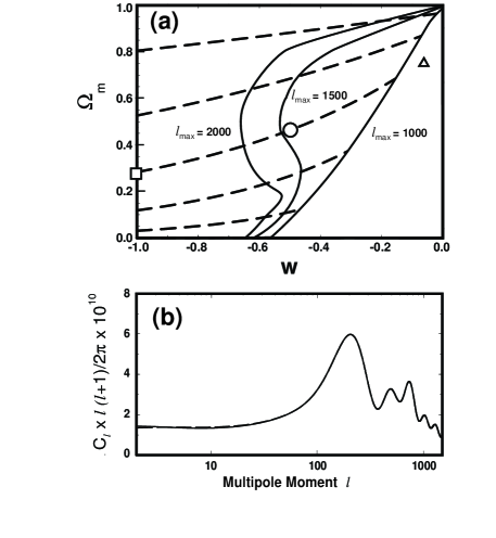
FIG. 1.: The CMB degeneracy problem: Each dashed curve in (a) represents a family of QCDM and $\Lambda$CDM models with indistinguishable CMB anisotropy power spectra. For an ideal, full-sky, cosmic variance limited experiment with $\ell_{\rm max}=1000,\,1500,\,2000$, the solid lines mark the projection of the right-most boundary of the degeneracy region. For example, Panel (b) shows two overlapping spectra for the $\Lambda$ (square) and quintessence (circle) models indicated in (a). Models beyond the solid line in (a) (e.g., the triangle for $\ell_{\rm max}=1000$, or the circle for $\ell_{\rm max}=2000$) are distinguishable.

Figure 1 illustrates the degeneracy problem for CMB anisotropy measurements. Figure 1a shows the $\Omega_{m}-w$ plane of quintessence models with a slowly varying or constant equation of state, where the axis $w=-1$ corresponds to the case of a cosmological constant. Each dashed curve represents a set of cosmological models with a $Q$- or $\Lambda$-component which satisfy the conditions for the geometric degeneracy for CMB anisotropy power spectra. The solid curves represent the projection of the right-most border of the degeneracy region, in the full parameter space, at which models can be distinguished from $\Lambda$CDM at the $\geq 3\sigma$ level, including the effect of lensing, for an idealized, cosmic variance limited experiment with a given maximum multipole moment. For example, for fixed $\Omega_{b}h^{2}$ and $n_{s}$ (the spectral index of scalar fluctuations), a model with quintessence and $\Omega_{m}=0.47$, $w=-1/2$ and $h=0.57$ (circle) produces a nearly identical CMB power spectrum to a $\Lambda$ model with $\Omega_{m}=0.29$, $w=-1$ and $h=0.72$ (square) for $\ell_{\rm max}=1000$. As the range of multipole moments increases, including smaller scale CMB anisotropy, the gravitational lensing distortion becomes more pronounced, breaking the geometric degeneracy. Yet we see that for many quintessence models, even with an ideal, cosmic variance limited, full-sky measurement of the CMB anisotropy with multipoles $\ell\leq 2000$, there remains a degeneracy in the $\Omega_{m}-w$ parameter space. We show Figure 1b to illustrate the extent of the degeneracy, as the two power spectra overlap almost entirely.

The degeneracy curves can be understood theoretically. They correspond approximately to the set of models that obey the following constraints: (a) $\Omega_{m}+\Omega_{Q}=A=1$; (b) $\Omega_{m}h^{2}=B$; (c) $\Omega_{b}h^{2}=C$; (d) $n_{s}=D$; and, (e) $\ell_{P}=E$. Here $A,B,C,D,E$ are constants, and $\ell_{P}$ is the multipole corresponding the position of the first acoustic (Doppler) peak. Constraint (a) is the flatness condition. Constraints (b)-(d) are required in order for the Doppler peak heights to remain constant. Along with constraint (d), we assume that $r$, the ratio of the tensor-to-scalar primordial power spectrum amplitudes obeys inflationary predictions.[21, 22] Constraint (e) insures that the acoustic peaks occur at the same multipole moment. The peak position $\ell_{P}$ (proportional to the ratio of the conformal time since last scattering to the sound horizon at last scattering) depends on $\Omega_{m}h^{2}$, $\Omega_{b}h^{2}$, $h$ and $w$. The only way to keep $\ell_{P}$ constant along the degeneracy curve as $w$ varies is to adjust $h$, since $\Omega_{m}h^{2}$ and $\Omega_{b}h^{2}$ are constrained to be fixed by (b) and (c). (M. White has independently noted similar conditions for degeneracy for constant $w$ models.[23]) Our results are based on full numerical codes which include the fluctuations in $Q$ and the gravitational lensing distortion[24]. Our computations confirm that the above conditions are a good approximation to the degeneracy curves. When we restrict our attention to $\ell\lesssim 1000$, angular scales on which lensing is negligible, then if the value of $h$ for the first model along the degeneracy curve is changed, the value of $h$ for the rest of the models can be adjusted so that the geometric degeneracy remains. The boundary of the $\ell_{\rm max}=1000$ degeneracy region is then determined by fluctuating $Q$ effects and the large integrated Sachs-Wolfe contribution to the CMB anisotropy, such that models with $w\gtrsim-\Omega_{Q}/2$ are distinguishable from $\Lambda$. At smaller angular scales, where lensing is important, raising or lowering $\Omega_{m}h^{2}$ results in increasing or decreasing the mass power spectrum, and therefore the strength of the lensing distortion. The question of what can be determined by the CMB alone becomes academic if we permit unphysically low values of $\Omega_{b}$ or $h$, in which case the effect of lensing becomes negligible. In determining this degeneracy region, then, we have permitted a conservative, physically-motivated range for the cosmological parameters, $h\geq 0.5$ and $\Omega_{b}h^{2}\in[0.016,0.024]$. This explains the shape of the $\ell_{\rm max}=1500,\,2000$ boundary; for the allowed range of cosmological parameters, the lensing is strong, breaking the degeneracy when the amplitude of the mass power spectrum and amplitude of acoustic oscillations are large. Note that the limiting cases $\Omega_{m}\to 1,\,0$ are special. In the former case, a negligible amount of quintessence is present, so that all QCDM models generate the same, degenerate CMB anisotropy pattern. In the latter case, as $\Omega_{m}\to\Omega_{b}$, the strength of the baryon-photon oscillations grows, compensating for the decrease in the mass power spectrum amplitude, so that lensing breaks the degeneracy.

A degeneracy curve represents the center of a strip of models in the $\Omega_{m}-w$ plane which cannot be distinguished by the CMB alone. To estimate the width of the degeneracy strip, we select a quintessence and $\Lambda$ model on a given degeneracy curve, vary $\Lambda$, and compute the likelihood that the quintessence model and the $\Lambda$ model are distinguishable, allowing for cosmic variance uncertainty. For each value of the cosmological constant $\Lambda$, the parameters $n_{s}$, $h$, $\Omega_{m}$ and $\Omega_{b}$ are varied until the likelihood is minimized. To compute the likelihood, a novel estimating procedure has been introduced which applies to more general examples of CMB analysis. The attractive feature is that the likelihood is simple to calculate analytically, avoiding the need for Monte Carlo. Suppose Models $A$ and $B$ are to be compared. We wish to estimate the likelihood that a Model $A$ real-sky would be confused as Model $B$. Since the prediction of Model $A$ is itself non-unique, subject to cosmic variance (and, in general, experimental error), we need to average the log-likelihood over the probability distribution associated with $A$. Only cosmic variance error, $C_{\ell}/\sqrt{2\ell+1}$, is assumed for each multipole $C_{\ell}$ and the distribution is chi-squared. In our notation, $C_{\ell}$’s are the cosmic mean values and $x_{\ell}$ are the values measured within our Hubble horizon. Then, the “average log-likelihood” is defined to be

$${\cal L}_{ba}=\int{\log\frac{{\cal P}(\{x_{\ell}\}|B)}{{\cal P}(\{x_{\ell}\}|A)}{\cal P}(\{x_{\ell}\}|A)dx_{1}\ldots dx_{\ell}\ldots}$$ (1)

where ${\cal P}(\{x_{\ell}\}|A)$ is the probability of observing the set of multipoles $\{x_{\ell}\}$ in a realization of Model $A$. Since each multipole $C_{\ell}$ from a full sky map is statistically independent, ${\cal P}(\{x_{\ell}\}|A)$ can be written as a simple product of chi-squared distributions for each $\ell$. Substituting the chi-square distribution for ${\em P}(x_{\ell}|A)$, ${\cal L}_{ba}$ reduces to

$${\cal L}_{ba}=-\sum_{\ell}(l+\frac{1}{2})\times(1-\frac{C_{\ell a}}{C_{\ell b}}+\log\frac{C_{\ell a}}{C_{\ell b}}).$$ (2)

Here we have assumed no experimental error, but it is a simple matter to include an additional experimental variance. Note that ${\cal L}_{ba}\neq{\cal L}_{ab}$ in general, although the difference is small in practice. We decide distinguishability according to the min(${\cal L}_{ba},\,{\cal L}_{ab}$). For variations $\Delta\Omega_{m}$ greater than $\pm 0.05$ from the degeneracy curve value, the log-likelihood satisfies $-{\cal L}\geq 6$, corresponding to distinguishability at the $3\sigma$ level or greater. This is the condition we use to determine distinguishability.

As long as only geometrical effects are important, distinguishability of a pair of cosmological models entails comparing the shapes of the two spectra without specifying any normalization. Once lensing and other non-linear effects are included, the absolute level of anisotropy must be specified; the shape of the $C_{\ell}$ spectrum is affected by the absolute scale of the mass power spectrum. Because the normalization is not known, some allowance must be made for this uncertainty in the lensing contribution. For the purposes of this investigation, we have assumed that for each pair of models, the mass power spectrum of the first model is COBE normalized,[25] while the spectrum of the second model must lie within $2\sigma$. A tighter constraint may arise from future satellite experiments, once the absolute level of anisotropy is known with better precision. It is interesting to note that despite the fact that the lensing tends to smear out sharp features in the CMB spectrum, effectively destroying information, we actually gain knowledge of the underlying mass power spectrum. As a result, the degeneracy region shrinks as the effect of lensing accumulates.

Now consider the situation in several years’ time, in which the CMB anisotropy measurements conform closely with one of the degeneracy curves in Figure 1a, a possibility consistent with current observations.[10] The degeneracy means that one cannot distinguish whether the missing energy is quintessence or vacuum energy. Furthermore, $\Omega_{m}$ and $h$ vary along the degeneracy curve (so as to keep $\Omega_{m}h^{2}$ constant), such that the uncertainty in these key parameters is very large. How can the ambiguities be resolved?

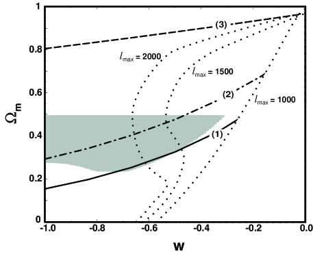
FIG. 2.: The CMB anisotropy constrains models to a particular degeneracy curve and, independently, provides tight constraints on $n_{s}$, $\Omega_{m}h^{2}$ and $\Omega_{b}h^{2}$. The latter constraints, along with other observational limits discussed in the text, fixes an allowed range of $\Omega_{m}$ and $w$ (the shaded region using the example discussed in the text). The combination determines the best-fit models.

Other cosmological observations may not be as precise as those of the CMB anisotropy, but they have the advantage that they do not share the same degeneracy. If other observations can be used to determine separately $\Omega_{m}$ or $h$ (or some combination of $\Omega_{m}$ and $h$ other than $\Omega_{m}h^{2}$), then perhaps the degeneracy between $\Lambda$ and quintessence can be broken. We have considered the current restrictions on $\Omega_{m}$ and $h$ obtained by combining the best limits on age ($>10$ Gyr), Hubble constant, baryon fraction ($\Omega_{b}h^{3/2}/\Omega_{m}\sim$ 3-10%), cluster abundance and evolution,[26] Lyman-$\alpha$ absorption,[27] deceleration parameter[28] and the mass power spectrum (APM Survey).[29] The current constraints and the techniques for combining them have been detailed elsewhere.[8, 10] We also include the fact that the CMB anisotropy will provide tight constraints on $n_{s}$ and the combinations $\Omega_{m}h^{2}$ and $\Omega_{b}h^{2}$ to within a few percent.[12, 13, 30, 31]

Even combining all the observational information listed above, $\Omega_{m}$ and $h$ are not highly constrained. Assume for illustrative purposes that the CMB anisotropy converges on $n_{s}=1$, $r=0$, $\Omega_{b}h^{2}=0.02$ and $\Omega_{m}h^{2}=0.15$ (reasonable values). Then Figure 2 shows the shaded region in the $\Omega_{m}$-$w$ plane which can satisfy the observational constraints at the $2\sigma$ level. In this case, acceptable models must lie at the overlap of the degeneracy curve picked out by the CMB anisotropy and the shaded region.

Three possibilities emerge, as shown in Figure 2: (1) the degeneracy curve overlaps the shaded region only over a limited range of $w$ so that the ambiguity between quintessence and $\Lambda$ is broken and $\Omega_{m}$, $h$ and $w$ are well-constrained; (2) the degeneracy curve cuts through the shaded region in such a way that a substantial ambiguity remains; or (3) the degeneracy curve and the shaded region do not overlap at all. Case (3) appears at first to be a contradiction: the CMB spectrum conforms to the predictions of a $\Lambda$CDM or QCDM model, but constraints from other cosmological observations (shaded region) suggest that the $\Omega_{m}$ is too small (or too big). However, this situation is precisely what ought to occur if one of our underlying assumptions is incorrect: namely, the flatness assumption, constraint (a). By introducing spatial curvature as an additional component ($A\neq 1$) further degeneracy arises. Associated with curve (3) is a continuous family of degeneracy curves in the $\Omega_{m}$-$w$ plane each beginning from a different value of $\Omega_{m}$ along the $w=-1$ axis.[12, 32] Making the universe open (closed) produces CMB degeneracy curves beginning with smaller (larger) values of $\Omega_{m}$, whereas the shaded region in Fig. 2 is only modestly changed. So, for example, curve (3) in Figure 2 is also degenerate with an open model with $\Omega_{m}=0.4$, $\Omega_{\Lambda}=0.54$ and $h=0.8$, which is consistent with the shaded region. Adding curvature is inconsistent with standard inflation-based models, but case (3) exemplifies how we may be forced observationally to consider the possibility.

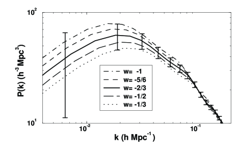
FIG. 3.: Mass power spectra for the models along the CMB degeneracy curve ($\Omega_{m}h^{2}=0.13$ and $\Omega_{b}h^{2}=0.02$) in Fig. 1a are difficult to distinguish with large-scale structure measurements. The error bars are projected standard errors (1$\sigma$) for SDSS assuming the middle ($w=-2/3$) curve.

The fact that Case (2) – continued degeneracy – remains possible after so much data has been invoked is remarkable. A reduction in experimental uncertainty ($\sigma$) by a factor of two for all of the measurements reduces the size of the shaded region in Fig. 2, but this is not sufficient to remove all possible degeneracy. For some constraints, much more than a factor of two improvement can be anticipated. For example, the Sloan Digital Sky Survey (SDSS) will provide a substantial improvement in measurements of the mass power spectrum $P(k)$ and velocities,[33, 34] especially on large lengths where $P(k)$ for models along the degeneracy curve are most different. Even so, as Figure 3 shows, the SDSS will not be enough to resolve the differences in the shape of $P(k)$ among models along the degeneracy curve. What would contribute immensely to the breaking of the degeneracy, rather, is an accurate determination of the mass power spectrum on scales $k\lesssim 0.1$ h/Mpc, where the models are most different.

It has been argued that combining the results of future Sloan and CMB experiments can lead to a substantial improvement in precision, isolating a narrow region of cosmological parameter space in order to distinguish between quintessence and Lambda.[20, 31] These improvements rely on the treatment of the errors as statistical and independent. We take a more conserative stance that the errors will be dominantly systematic. Hence, our conclusions are based on models passing the tests independently rather than by statistically combining the CMB and Sloan tests.

FIG. 4.: The magnitude-red shift relation may be a tool for distinguishing $\Lambda$ models (thick solid curve) from the family of quintessence models (dashed curves) along the degeneracy curve. $\Delta m$ is the difference in the predicted magnitude of a standard candle for a given model and an open universe ($\Omega_{m}\rightarrow 0$, middle dotted curve). The dashed curves are QCDM models with $w=-5/6,-2/3,-1/2,-1/3$ from top to bottom, respectively. Hypothetical type IA supernova data are shown at several red shift, assuming $w=-2/3$ with $1\sigma$ error bars of $\pm 0.1$ magnitudes. For reference, an $\Omega_{\Lambda}=1$ (upper dotted) and $\Omega_{m}=1$ (lower dotted) flat model are shown.

Figure 4 shows the prediction for the red shift luminosity relation, measured using Type IA supernovae as standard candles[28] for the same models along the degeneracy curve. In this case the quintessence models are more distinct from the $\Lambda$ model; however, it is premature to say whether observations will become accurate enough to make this measurable. Not only will a large number of high red shift SNe have to be observed, but the systematic errors in the magnitude calibration will have to be reduced, to $\Delta m\lesssim 0.1$, in order that a turn-over in $\Delta m$ is well determined.

One might expect that ground-based CMB experiments, which probe smaller angular scales than accessible by satellite experiments, can dramatically resolve the degeneracy problem. It is precisely on the small angular scales that non-linear effects such as gravitational lens distortion, the Rees-Sciama[35] and Ostriker-Vishniac[36] effects are important. However, these effects depend not only on the broad cosmological parameters $\Omega_{m},\,\Omega_{b},\,h$, but also on the details of re-ionization and small scale structure formation, about which there probably remains enough uncertainty to prevent this method from being used as a fine model discriminant. It is not clear whether such constraints, while sufficient to differentiate between $\Lambda$CDM and SCDM, can discriminate between quintessence and $\Lambda$.

Our conclusion is asymmetrical. A large class of quintessence models, those with rapidly varying $w$ or constant $w\gtrsim-\Omega_{Q}/2$, can be distinguished from $\Lambda$ models by near future CMB experiments such as MAP. However, any given $\Lambda$ model is indistinguishable from the subset of quintessence models along its degeneracy curve. CMB experiments which probe small angular scales where gravitational lens distortion is expected to be important, such as Planck, can be expected to cut into the degeneracy region. Combining the constraints which the CMB imposes on $n_{s}$, $\Omega_{m}h^{2}$ and $\Omega_{b}h^{2}$ to the other current observational constraints sometimes, but not always, breaks the degeneracy. Adding spatial curvature as an additional degree of freedom increases the degeneracy. Depending on how measurements overlap, new observational techniques must be invented to break the degeneracy.

We thank J. Bahcall, Wayne Hu, W. Press, J.P. Ostriker and M. Strauss for many useful comments. We thank M. Vogeley for explaining anticipated errors in SDSS and providing a code to estimate their magnitude. This research was supported by the Department of Energy at Penn, DE-FG02-95ER40893. We have modified the CMBFAST software routines[24] for our numerical computations.

REFERENCES

- [1]
- [2] map.gsfc.nasa.gov
- [3] astro.estec.esa.nl/SA-general/Projects/Planck/
- [4] A. Dekel, D. Burstein, and S. D. M. White, in Critical Dialogues in Cosmology, ed. Neil Turok (World Scientific: Singapore, 1997), p.175; Alan Guth, ibid, p.233; Marc Kamionkowski, Science 280, 1397 (1998).
- [5] S. Weinberg, Rev. Mod. Phys. 61, 1 (1989).
- [6] S. Carroll, W. H. Press, and E. L. Turner, Ann. Rev. Astron. & Astrophys. 30, 499 (1992).
- [7] L. Krauss and M. S. Turner, Gen. Rel. Grav. 27, 1137 (1995).
- [8] See, for example, J. P. Ostriker and P. J. Steinhardt, Nature (London) 377, 600 (1995), and references therein.
- [9] R. R. Caldwell, R. Dave and P. J. Steinhardt, Phys. Rev. Lett. 80, 1582 (1998).
- [10] L. Wang, R. R. Caldwell, J. P. Ostriker, and P. J. Steinhardt, in preparation.
- [11] R. R. Caldwell and P. J. Steinhardt, in The Non-Sleeping Universe, eds. Alain Blanchard and M. Teresa V.T. Lago (World Scientific: Singapore, 1998).
- [12] M. Zaldarriaga, D. Spergel, and U. Seljak, Astrophys. J. 488, 1 (1997).
- [13] J. R. Bond, G. Efstathiou and M. Tegmark, Mon. Not. R. Astron. Soc. 291 L33 (1997); G. Efstathiou and J. R. Bond, astro-ph/9807103.
- [14] A. Blanchard and J. Schneider, Astron. & Astrophys. 184, 1 (1987).
- [15] S. Cole and G. Efstathiou, Mon. Not. R. Astron. Soc. 239, 195 (1989).
- [16] L. Cayon, E. Martinez-Gonzalez, and J. L. Sanz, Astrophys. J. 403, 471 (1993); ibid 413, 10 (1993); ibid 489, 21 (1997).
- [17] U. Seljak, Astrophys. J. 463, 1 (1996).
- [18] R. Benton Metcalf and Joseph Silk, astro-ph/9708059; astro-ph/9710364.
- [19] R. Stompor and G. Efstathiou, astro-ph/9805294.
- [20] Wayne Hu, Daniel J. Eisenstein, Max Tegmark, and Martin White, astro-ph/9806362.
- [21] Richard L. Davis, Hardy M. Hodges, George F. Smoot, Paul J. Steinhardt, and Michael S. Turner, Phys. Rev. Lett. 69, 1856 (1992); Erratum, ibid, 70, 1733 (1993).
- [22] R. R. Caldwell and Paul J. Steinhardt, Phys. Rev. D 57, 6057 (1998).
- [23] M. White, astro-ph/9802295.
- [24] U. Seljak and M. Zaldarriaga, Astrophys. J. 469, 437 (1996); arcturus.mit.edu:80/matiasz/CMBFAST/cmbfast.html
- [25] E. F. Bunn and M. White, Astrophys. J. 480, 6 (1997).
- [26] Limin Wang and Paul J. Steinhardt, astro-ph/9804015.
- [27] J. Miralda-Escude, et al, in Proceedings of 13th IAP Colloquium: Structure and Evolution of the IGM from QSO Absorption Line Systems, eds. P. Petitjean, S. Charlot; astro-ph/9710230.
- [28] S. Perlmutter, et al, Nature (London) 391, 51 (1998); P. M. Garnavich, et al, astro-ph/9710123; Adam G. Riess, Peter Nugent, Alexei V. Filippenko, Robert P. Kirshner, and Saul Perlmutter, astro-ph/9804065.
- [29] J. Peacock, Mon. Not. R. Astron. Soc. 284, 885 (1997); private communication, 1997.
- [30] G. Jungman, M. Kamionkowski, A. Kosowsky, and D. N. Spergel, Phys Rev. D 54, 1332 (1996).
- [31] Daniel J. Eisenstein, Wayne Hu, and Max Tegmark, astro-ph/9807130.
- [32] G. Huey and R. Dave, unpublished report (1997).
- [33] M. S. Vogeley, in Wide-Field Spectroscopy and the Distant Universe, eds. S. J. Maddox & A. Aragón-Salamanca (World Scientific: Singapore, 1995), p. 142.
- [34] Max Tegmark, Andrew Hamilton, Michael Strauss, Michael Vogeley, and Alexander Szalay, Astrophys.J. 499, 555 (1998).
- [35] M. J. Rees and D. W. Sciama, Nature (London) 517, 611 (1968); Robin Tululie, Pablo Laguna, and Peter Anninos, Astrophys. J. 463, 15 (1996).
- [36] J. P. Ostriker and E. T. Vishniac, Astrophys. J. 306, L51 (1986); Andrew H. Jaffe and Marc Kamionkowski, astro-ph/9801022 (1998).