A new statistic for picking out Non-Gaussianity in the CMB

Abstract

In this paper we propose a new statistic capable of detecting non-Gaussianity in the CMB. The statistic is defined in Fourier space, and therefore naturally separates angular scales. It consists of taking another Fourier transform, in angle, over the Fourier modes within a given ring of scales. Like other Fourier space statistics, our statistic outdoes more conventional methods when faced with combinations of Gaussian processes (be they noise or signal) and a non-Gaussian signal which dominates only on some scales. However, unlike previous efforts along these lines, our statistic is successful in recognizing multiple non-Gaussian patterns in a single field. We discuss various applications, in which the Gaussian component may be noise or primordial signal, and the non-Gaussian component may be a cosmic string map, or some geometrical construction mimicking, say, small scale dust maps.

1 Introduction

Current theories of structure formation may be roughly divided into two classes: active and passive perturbations. According to the inflationary paradigm, quantum fluctuations in the very early universe are produced during a period of inflation [Steinhardt 1995] and grow to become classical density perturbations [Liddle & Lyth 1993, Bardeen 1980]. These perturbations evolve linearly until late times when the overdensities become galaxies. Perturbations due to inflation are called passive because they are seeded at some initial time near the Planck time and then evolve ‘deterministically’, or linearly. They leave their imprint on the CMB at last scattering [Peebles 1970, Hu, Sugiyama & Silk 1997, Hu & Sugiyama 1995a, Hu & Sugiyama 1995b, Battye 1997, White, Scott & Silk 1994]. Although this is not strictly necessary, in most cases the fluctuations in the CMB temperature due to inflationary perturbations form a Gaussian random field [Bond & Efstathiou 1987, Bardeen et al. 1986].

There is another class of theories of structure formation, topological defects caused by phase transitions in the early universe [Kibble 1980, Vachaspati & Vilenkin 1984]. Perturbations caused by defects are known as active perturbations [Magueijo et al. 1996, Albrecht 1996] since they are continually being seeded by an evolving network of defects through the history of the universe. The fluctuations in the CMB in defect models have been found to be non-Gaussian [Bouchet, Bennett & Stebbins 1988], even though the extent and strength of this non-Gaussianity is still far from clear. Recently a wide class of defect models have been shown to be in conflict with current data [Pen, Seljak & Turok 1997, Albrecht, Battye & Robinson 1997a, Albrecht, Battye & Robinson 1997b] but some viable active models still remain [Turok 1996, Durrer & Sakellariadou 1997, Albrecht et al. 1998]. In fact, some of the most interesting [Battye, Robinson & Albrecht 1997, Avelino et al. 1997] of these (based on cosmic strings) require a non-zero cosmological constant of the sort that currently favoured by supernova experiments [Perlmutter et al. 1998].

Thus it is important to be able to distinguish Gaussian from non-Gaussian fluctuations. Many different tests are being tried [Kogut et al. 1996, Luo 1994, Ferreira & Magueijo 1997, Ferreira, Magueijo & Silk 1997, Schmalzing & Gorski 1998, Winitzki & Kosowsky 1997], adapted to different experimental settings, and types of signal. Our statistic is designed to be used for small fields where one or more distinctive shapes are obscured by an extra Gaussian component, and so are not visible in real space. It is our experience in previous work [Ferreira & Magueijo 1997] that in such situations standard statistics, based in real space, fail to recognize the non-Gaussianity of the signal. The idea is to study the statistical properties of map derivatives which are only sensitive to a given scale. In this way we may separate out different scales, some of which may have Gaussian or nearly Gaussian fluctuations, some very non-Gaussian. Although this scale filtering may be achieved using the wavelet transform [Ferreira, Magueijo & Silk 1997, Pando & Fang 1996], in this paper we choose to use the Fourier transform as our scale filter.

One problem with this approach is that the Fourier transform is a global transformation, and therefore can only recognize non-Gaussian structures globally. It may therefore offer a rather contorted description for complicated networks made up of essentially simple objects. We will however perform a transformation over the Fourier modes: a second Fourier transform, in angle, for modes in each ring in Fourier space. We will argue that by doing so we are able to recognize mostly features of individual objects, and so bypass this problem. This operation returns a set of quantities which are blind to the random orientations of individual objects. Unfortunately their random positions still affect our statistic, so there will be a limit (albeit less stringent) on the number of objects in the field before our statistic becomes confused.

The plan of this paper is as follows. In Section II we look at some of the ideas involved in thinking about non-Gaussianity. In Section III we define our statistic and look at some of its properties and motivations. In Section IV we apply our statistic to practical situations in which subtle non-Gaussian signals are present. We consider non-Gaussian signals corrupted by the presence of a Gaussian process, which can be noise or primordial signal, and which dominates on all but a narrow band of scales. We consider two types of non-Gaussian signal. We consider CMB maps obtained from string simulations, implementing the algorithms in [Smith & Vilenkin 1987]. We also consider geometrical constructions mimicking, say, small scale dust maps. We show how such maps look very Gaussian, but fail to confuse our statistic.

2 Non-Gaussian Statistics

The fluctuations in the temperature of the radiation are described by $\frac{\Delta T}{T}({\mn@boldsymbol{n}})$ on a two-sphere. Generally this is expanded in spherical harmonics, but for small fields it can be expanded in Fourier modes:

$$\frac{\Delta T}{T}({\mn@boldsymbol{x}})={\int{{\rm d}^{2}{\mn@boldsymbol{k}}\over 2\pi}a({\mn@boldsymbol{k}}){\rm e}^{{\rm i}\mn@boldsymbol{k\cdot x}}}$$ (1)

The assumption of homogeneity and isotropy leads to the relation between Fourier modes

$$\langle a^{*}({\mn@boldsymbol{k}_{1}})a({\mn@boldsymbol{k}_{2}})\rangle=\delta({\mn@boldsymbol{k}_{1}}-{\mn@boldsymbol{k}_{2}})P(k_{2})$$ (2)

where $P(k)={\langle|a({\mn@boldsymbol{k}})|^{2}\rangle}_{|{\mn@boldsymbol{k}}|=k}$ is the power spectrum and the averages are ensemble averages.

Homogeneity means that $\langle|\frac{\Delta T}{T}({\mn@boldsymbol{x}})|^{2}\rangle=\langle|\frac{\Delta T}{T}({\mn@boldsymbol{x+b}})|^{2}\rangle$ for all vectors ${\mn@boldsymbol{b}}$ which means $\langle a^{*}({\mn@boldsymbol{k}}_{1})a({\mn@boldsymbol{k}}_{2})\rangle=0$ for ${\mn@boldsymbol{k}}_{1}\neq{\mn@boldsymbol{k}}_{2}$. Isotropy in real space corresponds to isotropy in Fourier space so the power spectrum can only depend on the modulus of ${\mn@boldsymbol{k}}$.

It is often assumed that the Fourier modes form a Gaussian random field. The real and imaginary parts of the Fourier modes of a Gaussian random field are drawn from a Normal distribution with mean zero and variance $P(k)/2$ which means that the phases are random and the moduli have a $\chi^{2}$ distribution. From our experience, we know that in real space a Gaussian random field has little structure. We may of course have a field that obeys equation (2) but which clearly has structure in real space, for example a field containing squares at random positions and orientations. This is clearly non-Gaussian. The important point is that the averages in equation (2) are ensemble averages, which do not necessarily convert to spatial or sample averages. For a non-Gaussian field we expect to have to take spatial averages over larger regions (or bigger samples) than for a Gaussian random field in order to get results which approximate equation (2).

There are various ways we can think about non-Gaussianity. The formal definition is the departure of the distribution of the modes from a Normal distribution. This includes cases where the phases of the Fourier modes are random and there is no structure in real space. If we assume the Fourier modes are independent then homogeneity implies that the modes have random (uniformly distributed) phases. By the central limit theorem the distribution rapidly becomes like a Gaussian as we increase the size of the field and spatial averages rapidly become good estimates of ensemble averages, i.e. the Fourier modes come close to satisfying equation (2). For these cases there will be little or no structure in real space.

In order to get structure in the field, we must therefore introduce correlations in the modes. This means that spatial averages will take longer to approach ensemble averages than for a Gaussian random field. This is because each realisation of the field has fewer independent modes than a Gaussian random field does. Therefore, to detect this type of non-Gaussianity we can test how well spatial averages obey equation (2) compared to a Gaussian random field, rather than looking at the actual distribution of Fourier modes. Here we choose to look at $a(\mn@boldsymbol{k})$ in a ring of constant $|{\mn@boldsymbol{k}}|\equiv k$ in Fourier space, to test the isotropy of spatial averages of the field.

Another reason for looking at the field in Fourier space is to detect non-Gaussian fluctuations superimposed on a Gaussian background. This happens for instance in cosmic string scenarios where the effects of strings on photons after last scattering (Kaiser-Stebbins effect [Kaiser & Stebbins 1984]) are superimposed on the fluctuations from before last scattering which can be considered to be Gaussian. The field may be non-Gaussian on some scales but Gaussian on others, making it hard to see the non-Gaussianity in real space. If there is more power from the non-Gaussian features than from the Gaussian on a particular scale this should show in Fourier space.

3 Another Fourier Transform

3.1 Definition

We can write the Fourier coefficients as

$$a({\mn@boldsymbol{k}})=\rho({\mn@boldsymbol{k}}){\rm e}^{{\rm i}\phi({\mn@boldsymbol{k}})}$$ (3)

Here we will focus on the amplitudes. As we are considering constant $k$ we will write

$$\rho({\mn@boldsymbol{k}})\equiv\rho_{k}(\alpha)$$ (4)

where $\alpha$ is the angle of the direction of $\mn@boldsymbol{k}$ in polar co-ordinates.

We take another Fourier transform in the angle $\alpha$ around the ring.

$$F_{k}(\beta)=\frac{1}{N}\sum_{n=0}^{N-1}{\rho^{2}_{k}(\alpha_{n}){\rm e}^{-{\rm i}{\alpha_{n}}{\beta}}}$$ (5)

For a completely isotropic field $\langle|a({\mn@boldsymbol{k}})|^{2}\rangle$ in one ring in Fourier space is constant i.e. $\langle\rho^{2}_{k}(\alpha)\rangle$ is constant in $\alpha$ so $\langle F_{k}(\beta)\rangle$ is a $\delta$-function in $\beta$.

3.2 Motivations: Repeated shapes

This statistic is motivated by the idea of detecting patterns or shapes that are repeated at different places. If one particular feature has a temperature pattern $f(\mn@boldsymbol{x})$ with Fourier transform $\tilde{f}(\mn@boldsymbol{k})$ and the field we are looking at consists of the feature repeated at $n$ different positions so the field in real space is

$$\frac{\Delta T}{T}({\mn@boldsymbol{x}})=\sum_{i=1}^{n}f({\mn@boldsymbol{x+b}}_{i})$$ (6)

then the Fourier transform of the whole field is

$$a({\mn@boldsymbol{k}})=\sum_{i=1}^{n}\tilde{f}({\mn@boldsymbol{k}}){\rm e}^{{\rm i}{\mn@boldsymbol{k}}\cdot{\mn@boldsymbol{b}}_{i}}$$ (7)

and the amplitude satisfies

$$\rho^{2}({\mn@boldsymbol{k}})=|\tilde{f}({\mn@boldsymbol{k}})|^{2}\left(n+2\sum_{i\neq j}\cos({\mn@boldsymbol{k}}\cdot({\mn@boldsymbol{b}}_{i}-{\mn@boldsymbol{b}}_{j}))\right)$$ (8)

The amplitude consists of an envelope defined by the Fourier transform of the individual feature together with oscillations which depend on the relative positions of the repeated features. The idea of taking the second Fourier transform is to get a similar envelope with oscillations in one dimension around the ring of constant modulus $k$.

As $n$ gets larger $\rho^{2}({\mn@boldsymbol{k}})\rightarrow n|\tilde{f}({\mn@boldsymbol{k}})|^{2}$ since the cosine averages to zero for many positions, so we can extract the Fourier transform of the original feature from the Fourier transform of the whole field. We can write this for each ring as $\rho_{k}^{2}(\alpha)\rightarrow n|\tilde{f}_{k}(\alpha)|^{2}$ so we see this applies to each ring also.

But if the shapes are repeated with different orientations, equation (8) becomes

$$\rho^{2}({\mn@boldsymbol{k}}) = \sum_{i}|\tilde{f}(R_{i}{\mn@boldsymbol{k}})|^{2}+2\sum_{i\neq j}\left[\left(\Re e\tilde{f}(R_{i}{\mn@boldsymbol{k}})\Re e\tilde{f}(R_{j}{\mn@boldsymbol{k}})\right.\right.$$ (9)

$$\left.\mbox{}+\Im m\tilde{f}(R_{i}{\mn@boldsymbol{k}})\Im m\tilde{f}(R_{j}{\mn@boldsymbol{k}})\right)\cos\left({\mn@boldsymbol{k}}\cdot({\mn@boldsymbol{b}}_{i}-{\mn@boldsymbol{b}}_{j})\right)$$

$$\mbox{}+\left(\Re e\tilde{f}(R_{i}{\mn@boldsymbol{k}})\Im m\tilde{f}(R_{j}{\mn@boldsymbol{k}})\right.$$

$$\mbox{}-\left.\left.\Im m\tilde{f}(R_{i}{\mn@boldsymbol{k}})\Re e\tilde{f}(R_{j}{\mn@boldsymbol{k}})\right)\sin\left({\mn@boldsymbol{k}}\cdot({\mn@boldsymbol{b}}_{i}-{\mn@boldsymbol{b}}_{j})\right)\right]$$

where the $\{R_{i}\}$ are the matrices of the rotations. As $n$ gets larger $\rho^{2}({\mn@boldsymbol{k}})\rightarrow\sum_{i}|\tilde{f}(R_{i}{\mn@boldsymbol{k}})|^{2}$ in a similar manner to before, which we can write as $\rho_{k}^{2}(\alpha)\rightarrow\sum_{i}|\tilde{f}_{k}(\alpha+\theta_{i})|^{2}$ where $\theta_{i}$ is the angle of the $i$th rotation. It is clear that in each ring this will actually tend to a constant (in $\alpha$) as n becomes large if the angles of the rotations are uniformly distributed. This is merely a consequence of the increasing isotropy of the field.

Even with just a few repeated shapes we cannot extract the original shape as we could in the case without rotations without knowing the number and orientations of the repeated shapes. But unless $n$ is very large $\rho_{k}^{2}(\alpha)$ should be distinguishable from a Gaussian. We know that these features will disappear when averages are taken over a large enough sample. The point is to get a statistic which will show the lack of homogeneity and isotropy on small scales and for small samples.

3.3 Averaging over small fields

Another way of using this statistic is to look at very small fields (i.e. those containing only a few shapes). To do statistics on these observations we want to look at many small fields. If we say look at several small fields each containing one shape but at different orientations (as we would expect from isotropy) then we will get the same Fourier transform rotated each time. Mathematically it is similar to the calculations leading to equation (9) except we don’t consider translations. The real space pattern in the $i$th field is $(\frac{\Delta T}{T})_{i}({\mn@boldsymbol{x}})=\frac{\Delta T}{T}(R_{i}{\mn@boldsymbol{x}})$ so the Fourier transform of the field satisfies $\rho^{2}_{i}({\mn@boldsymbol{k}})=\rho^{2}(R_{i}{\mn@boldsymbol{k}})$ which we write in one ring as

$$\rho^{2}_{k(i)}(\alpha)=\rho^{2}_{k}(\alpha+\theta_{i})$$ (10)

The Fourier transform taken in angle round the ring satisfies $F_{k(i)}(\beta)=F_{k}(\beta){\rm e}^{{\rm i}\theta_{i}\beta}$ so

$$|F_{k(i)}(\beta)|^{2}=|F_{k}(\beta)|^{2}$$ (11)

for each field.

Note that if we averaged over the original single-Fourier transformed fields $\{\rho^{2}_{k(i)}(\alpha)\}$ before taking the second Fourier transform we would get

$$|\sum_{i}F_{k(i)}(\beta)|^{2}=|F_{k}(\beta)|^{2}\left(n+2\sum_{i\neq j}\cos(\beta(\theta_{i}-\theta_{j}))\right)$$ (12)

which tends to a constant as we add more fields. We have to take the second Fourier transform of each field before averaging to see the non-Gaussianity. This is because the features in $\rho^{2}_{k}(\alpha)$ are repeated at different $\alpha$ in each field and their sum will tend to a constant for many fields. Taking the second Fourier transform takes the feature from $\rho^{2}_{k}(\alpha)$ and transforms it to a feature at the same $\beta$ in $F_{k}(\beta)$ for each field.

The idea of looking at small fields in this way is an extension of the idea in [Ferreira & Magueijo 1997] of analysing several small fields separately. For the example of a cosmic string on a Gaussian background used in [Ferreira & Magueijo 1997] the shape spectrum shows the non-Gaussian feature well, but the string was always considered to have the same orientation. If the shape spectrum were averaged over different directions the result would disappear. Here we can look at the same fields with different orientations and the non-Gaussianity will still be apparent. However, if we randomly choose small fields from a larger one containing many shapes we would have to take translations into account as well and the effect will not be so clear.

4 Applications

4.1 Geometric shapes

As a simple demonstration of this statistic on an obviously non-Gaussian field, we will consider applying it to some regular shapes. These are intended as mock small scale dust maps. We expect our geometric shapes to present the same type of non-Gaussianity, and obstacles for its detection, as the actual dust maps.

First to demonstrate the ideas in Section 3.3 we will look at fields each containing one square at different orientations. We first Fourier transform the whole field and take the amplitude squared ($\rho^{2}({\mn@boldsymbol{k}})$). For one square the amplitude is not affected by translation of the square. We multiply the field by a Gaussian window to get rid of edge effects [Hobson & Magueijo 1996].

In Figure 1 we have plotted for one field $\rho^{2}(\alpha)$ and $|F(\beta)|$ at $k=60$ from a $200^{2}$ array. This corresponds to a physical scale of $k=21600/L$ where $L$ is the size of the real field in degrees. The y-axis is in arbitrary units. Figure 2 shows the same functions averaged over 100 fields. The averaged $|F(\beta)|$ is not in fact identical to $|F(\beta)|$ for one field, because of numerical effects due to the discrete Fourier transform being on a lattice. The average settles down quickly, however: $|F(\beta)|$ looks the same averaged over 10 fields as it does averaged over 100 fields. The first Fourier transform, $\rho^{2}(\alpha)$, tends to a constant as we average over more fields as we would expect, but is also affected by the lattice.

Figure 1: First Fourier transform in one ring and modulus of second Fourier transform for a field containing 1 square.

Figure 2: Averages of the first and second Fourier transform from 100 realisations of a field containing 1 square.

Figures 3 and 4 show the equivalent graphs for a Gaussian random field. Here $|F(\beta)|$ converges rapidly and is distinct from the result for squares. The dips in $\rho^{2}(\alpha)$ are due to the window function superimposed in real space to avoid edge effects from the first Fourier transform. The Gaussian is treated in this way even though we generate the original map in Fourier space so as to model as closely as possible the way in which the non-Gaussian map is treated. We would of course expect $|F(\beta)|$ to tend to a delta function as the number of fields is increased but the window effects spoil this. The window used is in theory circularly symmetric but as it is on a lattice it necessarily has some squareness in it. The important point is that we get different results for the Gaussian and non-Gaussian fields.

Figure 3: First and second Fourier transforms for 1 realisation of a Gaussian random field.

Figure 4: Average of first and second Fourier transforms over 100 realisations of a Gaussian random field.

Now we test the statistic on fields with many squares. Figures 5 and 6 show the 1st and 2nd Fourier transforms for 10 and 100 squares in one field. We see that as the number of squares increases the result is not so distinctive. For 100 squares the signal is barely distinguishable from that of a Gaussian (see Figure 3). In fact in real space it is obviously not Gaussian, suggesting this is not the best way of detecting non-Gaussianity. Figure 7 shows the field in real space.

Figure 5: First and second Fourier transforms for 10 squares in one field.

Figure 6: First and second Fourier transforms for 100 squares in one field.

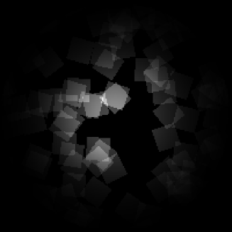
Figure 7: 100 squares in one field.

The important test however, is to see if we can detect non-Gaussianity when it is superimposed on a Gaussian background so it is not visible in real space. Figure 8 shows a real field which is the sum of a field containing one square and a Gaussian field. Though in real space we would not guess there was non-Gaussianity present, in fact in Fourier space many rings look different from those produced by Gaussian fields. An example of one is shown in Figure 9. This is the result of averaging over 10 such fields, as in Section 3.3, this time with a Gaussian background. Figure 10 shows the averages for 10 realisations of a Gaussian random field, for comparison. The characteristic signal of the square is still present.

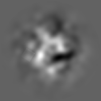
Figure 8: 1 square superimposed on a field of Gaussian fluctuations.

Figure 9: Average of first and second Fourier transforms for 10 realisations of 1 square superimposed on a Gaussian background.

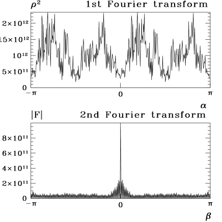
Figure 10: Average of first and second Fourier transforms for 10 realisations of a Gaussian.

4.2 Cosmic string maps

Finally we wish to see if this statistic could detect cosmic strings in the CMB. The work is motivated by this, since a simple approximation for a string map is to consider many string segments with random positions and orientations, and we hope the ideas illustrated above could apply. We will, however, use the results of string simulations to test the statistic.

The simulation gives us fields which have a physical size of $2\aas@@fstack{\circ}75$. The Fourier transform of the whole field appears Gaussian, so we look at small sections of the simulations to see if the statistic picks up the non-Gaussianity. We look at fields a quarter of the size of the simulation. We pick them at random, and analyse them individually. Figure 11 shows two graphs of $|F(\beta)|$ obtained from string maps. Again the y-axis is in arbitrary units. Many of the graphs obtained look similar to those obtained from Gaussian fields.

Figure 11: $|F(\beta)|$ for two different fields containing strings.

For each string simulation we first obtain $|F^{{\rm NG}}(\beta)|$, then generate 50 Gaussian fields with the same power spectrum as the string simulation and treat each one in exactly the same way as the string maps to obtain $|F^{{\rm G}}_{i}(\beta)|$, $i=1,...,50$. These 50 values of $|F^{{\rm G}}_{i}(\beta)|$ are used to obtain the sample variance for each $\beta$:

$$\sigma(\beta)=\sqrt{\frac{1}{N}\sum_{i}(|F^{{\rm G}}_{i}(\beta)|-|\overline{F}^{{\rm G}}(\beta)|)^{2}}$$ (13)

where $|\overline{F}^{{\rm G}}(\beta)|=\frac{1}{N}\sum_{i}|F^{{\rm G}}_{i}(\beta)|$.

Figure 12 shows the number of simulations giving a value of $|F(\beta)|$ above or below $|\overline{F}^{{\rm G}}(\beta)|\pm\sigma(\beta)$ for each $\beta$, for Gaussian fields and for fields containing strings. The total number of string simulations is 20 and the total number of Gaussian simulations is 1000. The axes are scaled so that the proportion of simulations giving values outside $|\overline{F}^{G}(\beta)|\pm\sigma(\beta)$ can be directly compared. Clearly the proportion is higher for the string simulations, i.e. $|F(\beta)|$ varies more. Large non-zero values of $\beta$ give more variation in $|F(\beta)|$ than values close to zero.

Figure 12: Number of simulations giving values of $|F(\beta)|$ outside $|\overline{F}^{{\rm G}}(\beta)|\pm\sigma(\beta)$ for Gaussian fields and fields containing strings.

We also want to see if we can detect the strings when they are covered in real space by Gaussian fluctuations. We have repeated the above procedure for string simulations superimposed on a Gaussian field. We have used a power spectrum with an exponential fall off on small scales as a simple model of the Gaussian fluctuations from before last scattering: $l(l+1)C_{l}\sim\exp({-(l/1200)^{2}})$ with the amplitude of the Gaussian fluctuations being twice that of the non-Gaussian fluctuations at $l=500$. This power spectrum can be considered to include noise if it is uncorrelated with the signal. This time the results are not so clear. Figure 13 shows the same graphs for string simulations superimposed on Gaussian simulations. Comparing the bottom graph to the top one would not convince us that it came from a non-Gaussian field.

Figure 13: Number of simulations giving values of $|F(\beta)|$ outside $|\overline{F}^{{\rm G}}(\beta)|\pm\sigma(\beta)$ for Gaussian fields and fields containing strings superimposed on Gaussian fields.

Analysing the data further, however, we can differentiate between the two cases. Figure 14 shows the number of simulations giving values of $|F(\beta)|$ $\it{below}$ $|\overline{F}^{{\rm G}}(\beta)|-\sigma(\beta)$, for Gaussian fields, and for strings and Gaussian superimposed fields. For many values of $\beta$, the proportion of $|F(\beta)|$ from non-Gaussian fields below $|\overline{F}^{{\rm G}}(\beta)|-\sigma(\beta)$ is higher than the proportion that we would expect from Gaussian fields. (This is also true for the strings only case, in fact most of the time in that case the values of $|F(\beta)|$ which are outside the ‘one sigma’ range lie below the lower one rather than above the upper one.)

Figure 14: Number of simulations giving values of $|F(\beta)|$ below $|\overline{F}^{{\rm G}}(\beta)|-\sigma(\beta)$ for Gaussian fields and fields containing strings superimposed on Gaussian fields.

So to test the sky for non-Gaussianity we need to look at several fields, generating Gaussian fields with the same power spectrum for each one, and see how many of the fields we are interested in give values of $|F(\beta)|$ below $|\overline{F}^{{\rm G}}(\beta)|-\sigma(\beta)$. Of course we need to look at a reasonable number of potentially non-Gaussian fields in order to see if the proportion is more than we would expect from Gaussian fields.

5 Discussion

We have introduced a statistic to look for non-Gaussianity in the cosmic microwave background. It is designed to pick out non-Gaussian features which are superimposed on Gaussian fluctuations and which are therefore not visible in real space. Since some scales may be more non-Gaussian than others we choose to separate them out. It is our experience in previous work [Ferreira & Magueijo 1997] that in such situations standard statistics, based in real space, fail to recognize the non-Gaussianity of the signal.

Our statistic is naturally tailored for interferometric experiments, which make measurements in Fourier space. Indeed the algorithm exposed above could easily be turned into a data analysis package operating over visibilities.

One of the problems with Fourier space statistics is that they recognize only global shapes. Therefore they become very ineffective when many individual structures are present. By taking another Fourier transform, in angle, over modes in a given ring in Fourier space, we can factor out orientations, and be only sensitive to an average shape of individual structures. Their random positions, on the other hand, will eventually make our statistic very ineffective as the number of objects becomes large. We found that although we have improved on previous work, still there is a limit on how many individual structures there may be in the field before the statistic fails to pick out their non-Gaussianity.

Finally, some comments are in order regarding the applications we have considered. The Gaussian component we have considered may include noise, if it has the right power spectrum. Hence we have already considered the effects of a simplified form of noise: it will merely reduce the band of scales where the non-Gaussian signal dominates, typically providing it with an upper boundary. An exception is the case of non uniform noise in the u-v plane, present in most interferometer experiments. Non uniform noise in the Fourier domain will look non-Gaussian, for it is a Gaussian process which is not isotropic or translationally invariant. Therefore an extra element of confusion, not dealt with in this paper, will appear.

Regarding the non-Gaussian component we have considered two types of signal. We have looked at some of the properties of the statistic when it is applied to a field containing one or more distinct shapes. The geometrical constructions presented are somewhat reminiscent of the jagged structures present in small scale dust maps. Experimenting on fields containing many structures we saw our statistic rapidly become blind to their non-Gaussianity. However interferometer fields are often small. They would therefore contain only a few, but more than one, of these structures. This is something our statistic can cope with, unlike previous Fourier space based statistics.

We have also studied our statistic when applied to cosmic string maps. We found that some individual small fields showed non-Gaussianity in the signal. If the results were averaged over many fields the effect of non-Gaussianity on $|F(\beta)|$ would not show. Once again this strategy is ideal for interferometers, for which combining small fields into a large field is in fact a rather awkward operation.

References

- [Albrecht 1996] Albrecht A. 1996, Coherence and Sakharov Oscillations in the Microwave Sky, in Proceedings of the XXXIst Recontre de Moriond, ’Microwave Anisotropies’.
- [Albrecht, Battye & Robinson 1997a] Albrecht A., Battye R. A. and Robinson J. 1997a, Phys. Rev. Lett., 79, 4736
- [Albrecht, Battye & Robinson 1997b] Albrecht A., Battye R. A. and Robinson J. 1997b, Phys. Rev. D, submitted
- [Albrecht et al. 1998] Albrecht A., Battye R. A., Robinson J. and Weller J. 1998, in preparation
- [Avelino et al. 1997] Avelino P. P., Shellard E. P. S., Wu J. H. P. and Allen B. 1997, preprint
- [Bardeen 1980] Bardeen J. M. 1980, Phys. Rev. D, 22, 1882
- [Bardeen et al. 1986] Bardeen J. M., Bond J. R., Kaiser N. and Szalay A. S. 1986, ApJ, 304, 15
- [Battye 1997] Battye R. A. 1997, Phys. Rev. D, 55, 7361
- [Battye, Robinson & Albrecht 1997] Battye R. A., Robinson J. and Albrecht A. 1997, preprint
- [Bond & Efstathiou 1987] Bond J. R. and Efstathiou G. 1987, MNRAS, 226, 655
- [Bouchet, Bennett & Stebbins 1988] Bouchet F. R., Bennett D. P. and Stebbins A. 1988, Nature, 335, 410
- [Durrer & Sakellariadou 1997] Durrer R. and Sakellariadou M. 1997, Phys. Rev. D, 56, 4480
- [Ferreira & Magueijo 1997] Ferreira P. G. and Magueijo J. 1997, Phys. Rev. D, 55, 3358
- [Ferreira, Magueijo & Silk 1997] Ferreira P. G., Magueijo J. and Silk J. 1997, Phys. Rev. D, 56, 4592
- [Hobson & Magueijo 1996] Hobson M. P. and Magueijo J. 1996, MNRAS, 283, 1133
- [Hu & Sugiyama 1995a] Hu W. and Sugiyama N. 1995a, ApJ, 444, 489
- [Hu & Sugiyama 1995b] Hu W. and Sugiyama N. 1995b, Phys. Rev. D, 51, 2599
- [Hu, Sugiyama & Silk 1997] Hu W., Sugiyama N. and Silk J. 1997, Nature, 386, 37
- [Kaiser & Stebbins 1984] Kaiser N. and Stebbins A. 1984, Nature, 310, 391
- [Kibble 1980] Kibble T. W. 1980, Phys. Rep., 67, 183
- [Kogut et al. 1996] Kogut A., Banday A. J., Bennett C. L., Gorski K., Hinshaw G., Smoot G. F. and Wright E. L. 1996, ApJ, 464, L29
- [Liddle & Lyth 1993] Liddle A. R. and Lyth D. H. 1993, Phys. Rep., 231, 1
- [Luo 1994] Luo X. 1994, Phys. Rev. D, 49, 3810
- [Magueijo et al. 1996] Magueijo J., Albrecht A., Ferreira P. G. and Coulson D. 1996, Phys. Rev. D, 54, 3727
- [Pando & Fang 1996] Pando J. and Fang L. Z. 1996, preprint
- [Peebles 1970] Peebles P. J. E. and Yu J. T. 1970, ApJ, 162, 815
- [Pen, Seljak & Turok 1997] Pen U. L., Seljak U. and Turok N. 1997, Phys. Rev. Lett., 79, 1615
- [Perlmutter et al. 1998] Perlmutter S. et al. 1998, Nature, 391, 51
- [Schmalzing & Gorski 1998] Schmalzing J. and Gorski K. M. 1998, MNRAS, in press
- [Smith & Vilenkin 1987] Smith A. G. and Vilenkin A. 1987, Phys. Rev. D, 36, 990
- [Steinhardt 1995] Steinhardt P. J. 1995, in Particle and Nuclear Astrophysics and Cosmology in the Next Millenium, ed. E. W. Kolb and R. Peccei (Singapore: World Scientific) 51
- [Turok 1996] Turok N. 1996, Phys. Rev. Lett., 77, 4138
- [Vachaspati & Vilenkin 1984] Vachaspati T. and Vilenkin A. 1984, Phys. Rev. D, 30, 2036
- [White, Scott & Silk 1994] White M., Scott D. and Silk J. 1994, ARA&A, 32, 319
- [Winitzki & Kosowsky 1997] Winitzki S. and Kosowsky A. 1997, New Astronomy, Vol. 3, No. 2, 75