NUMERICAL INVESTIGATIONS OF WEAK LENSING BY LARGE-SCALE STRUCTURE

We use numerical simulations of ray tracing through N-body simulations to investigate weak lensing by large-scale structure. These are needed for testing the analytic predictions of two-point correlators, to set error estimates on them and to investigate nonlinear gravitational effects in the weak lensing maps. On scales larger than 1 degree gaussian statistics suffice and can be used to estimate the sampling, noise and aliasing errors on the measured power spectrum. For this case we describe a minimum variance inversion procedure from the 2-d to 3-d power spectrum and discuss a sparse sampling strategy which optimizes the signal to noise on the power spectrum. On degree scales and smaller the shear and convergence statistics lie in the nonlinear regime and have a non-gaussian distribution. For this regime ray tracing simulations are useful to provide reliable error estimates and calibration of the measurements. We show how the skewness and kurtosis can in principle be used to probe the mean density in the universe, but are sensitive to sampling errors and require large observed areas. The probability distribution function is likely to be more useful as a tool to investigate nonlinear effects. In particular, it shows striking differences between models with different values of the mean density $\Omega_{m}$.

1 Introduction

Weak lensing by large-scale structure (LSS) shears the images of distant galaxies. The first calculations of weak lensing by LSS (Blandford et al. 1991; Miralda-Escude 1991; Kaiser 1992), based on the pioneering work of Gunn (1967), showed that lensing would induce coherent ellipticities of order 1$\%$ over regions of order one degree on the sky. Recently several authors have extended this work to probe semi-analytically the possibility of measuring the mass power spectrum and cosmological parameters from the second and third moments of the induced ellipticity or convergence (e.g. Bernardeau et al. 1997; Jain and Seljak 1997; Schneider et al. 1997).

The analytical work cited above suggested that nonlinear evolution of the density perturbations that provide the lensing effect can significantly alter the predicted signal. It enhances the power spectrum on scales below one degree and makes the probability distribution function (pdf) of the ellipticity and convergence non-Gaussian. We have carried out numerical simulations of ray tracing through N-body simulation data to compute the fully nonlinear moments and pdf. Details of the method and results are presented in a forthcoming paper; here we summarize the method and present some highlights of the results in Figures 1-5. We also discuss reconstruction of the dark matter power spectrum and error estimation using the gaussian approximation.

2 Ray Tracing Method

The dark matter distribution obtained from N-body simulations of different models of structure formation is projected on to 2-dimensional planes lying between the observer and source galaxies. Typically we use galaxies at $z\sim 1$ with $\sim 20-30$ planes. We propagate $\sim 10^{6}$ light rays through these planes by computing the deflections due to the matter at every plane. Fast Fourier Transforms are used to compute gradients of the potential that provide the shear tensor at each plane. The outcome of the simulation is a map of the shear and convergence on square patches of side length $1-5^{\circ}$. Several realizations for each model are needed to compute reliable statistics on scales ranging from $1^{\prime}$ to 1^∘. Figure 1 shows the shear map from two cold dark matter models with shape paratemeter $\Gamma=0.2$, one with $\Omega_{m}=1$ (upper panel) and the other with $\Omega_{m}=0.3$ (lower panel).

Numerical resolution on small scales is limited primarily by (i) the force softening used in the N-body simulations, and, (ii) by the finite size of the grid used to compute FFT’s and to propagate the light rays. We have chosen grid spacings in order to avail of the full resolution provided by the N-body simulations. The simulations used, adaptive $P^{3}M$ simulations with $256^{3}$ particles, were carried out using codes kindly made available by the Virgo consortium (e.g. Jenkins et al. 1997) and have previously been analyzed in the strong lensing regime by Bartelmann et al. (1998). These, coupled with ray tracing on a $2048^{2}$ grid, provide us with small scale resolution down to $\lower 2.15277pt\hbox{$\;\buildrel<\over{\sim}\;$}0.5^{\prime}$, well into the nonlinear regime for weak lensing. On large scales the finite number of transverse modes of the density field at any redshift leads to fluctuations that must be averaged using several realizations of the ray tracing as well as the N-body simulation for a given model. We have used an ensemble of $PM$ simulations to get reliable statistics on large scales.

In the weak lensing regime, the magnification and induced ellipticity are given by linear combinations of the Jacobian matrix of the mapping from the source to the image plane. The Jacobian matrix is defined by

$$\Phi_{ij}\equiv{\partial\delta\theta_{i}\over\partial\theta_{j}}$$ (1)

where $\delta\theta_{i}$ is the $i-$th component of the perturbation due to lensing of the angular position on the source plane, and $\theta_{j}$ is the $j-$th component of the position on the image plane. The convergence is defined as $\kappa=-(\Phi_{11}+\Phi_{22})/2$, while the two components of the shear are $\gamma_{1}=-(\Phi_{11}-\Phi_{22})/2$ and $\gamma_{2}=-\Phi_{12}$. The convergence $\kappa$ can be reconstructed from the measured shear $\gamma_{1}$, $\gamma_{2}$, up to a constant which depends on the mean density in the survey area. If the survey is sufficiently large and there is little power on scales larger than the survey, this error can be neglected.

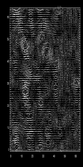
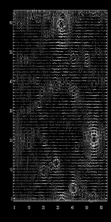
Figure 1: The shear pattern on a 1^∘ field for an Einstein-de Sitter model (upper panel) and an open model (lower panel) with $\Omega_{m}=0.3$. The rms shear in these fields is about $2\%$. The open model produces a shear pattern dominated mostly by halos of clusters or groups. The Einstein-de Sitter model has a lower normalization ($\sigma_{8}=0.6$) compared to the open model ($\sigma_{8}=0.85$) and evolves more rapidly with redshift – this leads to a smaller fraction of the mass being part of massive collapsed halos. The qualitative differences between the models are reflected in the statistical measures shown in the following figures.

3 Results of Simulations

Figure 2: The dimensionless power spectrum of $\kappa$ and $\gamma$. For the cosmological model indicated by $\Omega_{m}$ and $\Gamma$ in the panel, the power spectrum from ray tracing is compared with the linear (long-dashed) and nonlinear analytical (short-dashed) predictions. The dotted curves in two of the panels show measurements from individual realizations while the solid curves are the mean spectra. The angular wavenumber $l$ is given in inverse radians – the smallest $l$ plotted corresponds to modes with wavelength of order $L\simeq 2.5^{\circ}$, where $L$ is the side-length of the field. Note that the decline in the N-body power spectrum at $l>10^{4}$ is because of the limited resolution.

There are strong features due to the nonlinear clustering of the dark matter as shown in Figure 1. Collapsed halos produce tangential patterns of shear around them, while quasilinear filamentary structures are also visible. The two cosmological models show qualitative differences in the shear pattern, with the open model being far more dominated by halos and lacking irregular or filamentary structures. Figure 2 shows the power spectrum of the convergence (essentially identical to that of the shear) for 3 cosmological models. The amplitude of the convergence is enhanced by a factor of several compared to linear theory on small scales, as seen from the difference between the measured spectrum and the one predicted from linear theory. For a square field $2.5^{\circ}$ on a side essentially all the modes have become nonlinear. The analytical nonlinear spectrum (from Jain and Seljak 1997) agrees adequately (to about $20\%$) with the measured one over more than 2 orders of magnitude. On the smallest scales, the measured spectrum is suppressed due to resolution effects. For the middle panel there are differences with the analytic prediction caused by too small a simulation box (85$h^{-1}$Mpc). We ran several $PM$ simulations and found that for models with a lot of large scale power simulation boxes of size 200$h^{-1}$Mpc are needed for an adequate treatment of the large scale modes. The results from these simulations agree well with the analytic predictions.

Figure 3 shows the skewness and kurtosis of the convergence. The skewness on scales $\lower 2.15277pt\hbox{$\;\buildrel<\over{\sim}\;$}10^{\prime}$ is larger than the perturbation theory predictions shown by the dashed lines. The ratio of the skewness for the open and $\Omega_{m}=1$ models shows that it is a sensitive probe of matter density $\Omega_{m}$ (Bernardeau et al. 1997), but for a proper calibration one has to resort to N-body simulations. The kurtosis shows the same trend of increasing with decreasing $\Omega_{m}$. However the skewness and kurtosis are sensitive to the sampling variance and therefore require a large survey area for a robust measurement.

We also investigate the one-point pdf of the convergence and shear to assess its sensitivity to different model parameters. One example is shown in Figure 4, where the pdf of $\kappa$ is compared with that of the 3-dimensional overdensity $\delta=(\rho-\bar{\rho})/\bar{\rho}$. The comparison illustrates a key difference: whereas the pdf of $\delta$ is fully determined by the smoothed variance (for a given shape of the power spectrum), that of $\kappa$ is sensitive to $\Omega_{m}$ as well. The sensitiviy of the pdf and higher moments to $\Omega_{m}$ arises because the relative deflection of photons is determined by the projected matter density, not the relative overdensity. Particularly robust is the difference between the mean convergence, tracing the mean projected density, and the smallest negative convergence, tracing empty regions of the universe. In this case empty voids in an open universe produce a smaller de-magnification relative to the mean than in an $\Omega_{m}=1$ universe. This shows up as a less negative cut-off in the pdf in Figure 4 and, unlike the moments of pdf, is independent of the amplitude and shape of the power spectrum on sufficiently small scales. This difference at large negative $\kappa$ as well as differences in the positive tail account for the sensitivity of the pdf to $\Omega_{m}$. A detailed analysis of the pdf in the presence of noise will be given in a future publication.

Figure 3: The skewness $S_{3}(\theta)$ of $\kappa$ versus $\theta$ for low and high $\Omega_{m}$ models. The symbols in the upper panels show the skewness measured from four different realizations of the ray tracing. The solid line is the average over these realizations, while the dashed line is the prediction from perturbation theory. The lower left panel shows the ratio of the skewness for $\Omega_{m}=0.3$ and $\Omega_{m}=1$, again for the different realizations and their average. The lower right panel shows the kurtosis of $\kappa$ for the $\Omega_{m}=0.3$ model (triangles) and the $\Omega_{m}=1$ model (circles).

Figure 4: The probability distribution function (pdf) of $\kappa$ and of $\delta$, the 3-dimensional over-density. The left panel show the pdf of $\kappa$ for the open (dashed) model and the Einstein-de Sitter (solid) model. The thick solid curve uses the same smoothing scale as the dashed curve, $0.4^{\prime}$. The thin solid curve is for a smoothing scale of $1.6^{\prime}$ which has the same rms as the dashed curve. The right panel shows the pdf of the 3-dimensional density for the same two models, smoothed on a scale of 2.7 $h^{-1}$ Mpc. The rms for the two models is nearly the same. A comparison of the two panels shows that the rms completely dictates the pdf for $\delta$ (for the same shape of the power spectrum), while the pdf of $\kappa$ differs with $\Omega_{m}$ even if the rms is the same.

4 Power Spectrum Estimation

The first measure we want to extract from the observed data is the power spectrum in the presence of noise. On large scales (above one degree) the data are gaussian distributed and there is a well defined strategy to measure the power spectrum, which at the same time also provides the sampling and noise error estimate (Seljak 1997). On small scales the optimal weighting of the data is less critical, but one needs to use the N-body simulations to measure the sampling variance and mode-mode correlations.

On almost all the scales from a few arcminutes to several degrees the signal to noise in the power spectrum is much larger than unity for a survey of degree size and flux limit of I=25-26 (Jain & Seljak 1997). This suggests sparse sampling (Kaiser 1997), where the survey area is not fully covered, so that for a given amount of observing time the area can be increased (thereby reducing the sampling variance), while the density of galaxies is decreased (increasing the noise variance). If there was only noise then one could devise an optimal sampling strategy by equating the noise and sampling variance terms in the error matrix for the power spectrum. In practice however there is an additional noise term arising from the small scale modes that are not well measured. This aliasing term (see Seljak 1997 for its explicit form) is really a signal, but if those modes are not sufficiently well sampled, then they cannot be reconstructed and therefore act as noise. This additional power has to be added to the usual noise. If the sampling is sufficiently sparse, then this term dominates over the usual noise. Since its amplitude depends on the amount of small scale power one has to measure it first before subtracting its contribution.

This leads to the following adaptive sparse sampling strategy: first one measures the power on small scales using a filled survey. Once this power is measured to sufficient accuracy one can start to sparsely sample the sky, moving from smaller to larger and larger scales. At each step one minimizes the variance, which amounts to equating the sampling variance to the noise+aliasing variance, the later being estimated using the measured power on smaller scales. If the amount of small scale power is small one can afford very spase sampling, otherwise only modest sparse sampling can be used. In either case the formalism allows for an optimal sampling strategy which is adaptive in the sense that if the slope of the power spectrum changes as a function of scale so does the sampling fraction.

A $10^{\circ}\times 10^{\circ}$ field which is sparsely sampled gives a 2-d power spectrum shown in figure 5a. Usually one is more interested in a 3-d power spectrum and would therefore like to invert the 2-d to a 3-d spectrum. In general the 2-d power spectrum at some $l$ mode receives contributions from a wide range of 3-d $k$ modes, with the window peaking at $l\sim kr$, where $r$ is half the distance between the observer and the source galaxies. Conversely each 3-d spectral bin estimate will receive contributions from a range of 2-d spectral bins, appropriately weighted with the window so that 2-d bins close to the peak of the window have a larger weight than those far in the tails. In addition, one must also appropriately weight the 2-d estimators themselves using the corresponding covariance matrix. If a given 2-d bin has large sampling or noise variance then it should be downweighted appropriately. The complete formalism is presented in Seljak (1997). Figure 5b shows for the $10^{\circ}\times 10^{\circ}$ sparsely sampled field the 3-d reconstructed power spectrum. The reconstructed 3-d bins are strongly correlated because of the window. This explains why the variance on individual estimators is smaller than in the 2-d case – the estimators were essentially averaged over a wider range in $k$. This causes no problems if the power spectrum is smooth; however, fine details such as bumps and peaks cannot be accurately resolved with weak lensing data because of the smoothing. Note that we have assumed gaussian sampling variance, which becomes invalid on small scales ($k>0.5hMpc^{-1}$) and will increase the errors in that regime.

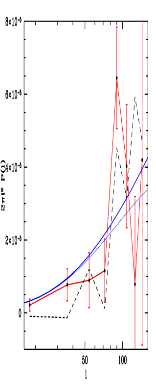
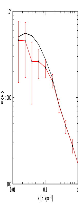
Figure 5: 2-d power spectrum reconstruction (left) and 3-d power spectrum reconstruction from the 2-d power spectrum (right). Both are for simulated 100 square degree sparsely (1 in 4) sampled data with a density of $2\times 10^{5}$ galaxies per square degree. The thick and thin solid lines on the left are for the nonlinear and linear power spectrum, respectively, while the dashed line is the power spectrum with $45^{\circ}$ rotation. The latter should vanish in a perfect survey if weak lensing signal is generated by gravity. If the sampling is sparse aliasing mixes power into this combination. The amount of aliasing can be estimated once the true power is measured, in which case on can verify the assumption of weak lensing signal generated by gravity. On the right the solid line is the nonlinear 3-d power spectrum. A survey of this size can reconstruct the power spectrum up to the turnover scale.

References

References

- [1] Bartelmann, M. et al. 1998, A&A, 330, 1
- [2] Bernardeau, F., van Waerbeke, L., & Mellier, Y. 1997, A&A, 322, 1
- [3] Blandford, R. D., Saust, A. B., Brainerd, T. G., & Villumsen, J. V. 1991, MNRAS, 251, 600
- [4] Gunn, J. E. 1967, ApJ, 147, 61
- [5] Jain, B., & Seljak, U., 1997, ApJ, 484, 560
- [6] Jenkins, A. et al. (The Virgo Consortium) 1997, astro-ph/9709010
- [7] Kaiser, N. 1992, ApJ, 388, 272
- [8] Kaiser, N. 1998, ApJ, in press, astro-ph/9610120
- [9] Miralda-Escude, J. 1991, ApJ, 380, 1
- [10] Schneider, P. et al. 1997, astro-ph/9708143
- [11] Seljak, U. 1997, astro-ph/9711124