A Unifying View of the Spectral Energy Distributions of Blazars

Abstract

We collect data at well sampled frequencies from the radio to the $\gamma$–ray range for the following three complete–samples of blazars: the Slew Survey and the 1 Jy samples of BL Lacs and the 2 Jy sample of Flat Spectrum Radio–Loud Quasars (FSRQs). The fraction of objects detected in $\gamma$–rays (E ${{}_{>}\atop{}^{\sim}}100$ MeV) is $\sim$ 17 %, 26 % and 40 % in the three samples respectively. Except for the Slew Survey sample, $\gamma$–ray detected sources do not differ either from other sources in each sample, nor from all the $\gamma$-ray detected sources, in terms of the distributions of redshift, radio and X–ray luminosities and of the broad band spectral indices (radio to optical and radio to X–ray).

We compute average spectral energy distributions (SEDs) from radio to $\gamma$–rays for each complete sample and for groups of blazars binned according to radio luminosity, irrespective of the original classification as BL Lac or FSRQ.

The resulting SEDs show a remarkable continuity in that: i) the first peak occurs in different frequency ranges for different samples/ luminosity classes, with most luminous sources peaking at lower frequencies; ii) the peak frequency of the $\gamma$–ray component correlates with the peak frequency of the lower energy one; iii) the luminosity ratio between the high and low frequency components increases with bolometric luminosity.

The continuity of properties among different classes of sources and the systematic trends of the SEDs as a function of luminosity favor a unified view of the blazar phenomenon: a single parameter, related to luminosity, seems to govern the physical properties and radiation mechanisms in the relativistic jets present in BL Lac objects as well as in FSRQ. The general implications of this unified scheme are discussed while a detailed theoretical analysis, based on fitting continuum models to the individual spectra of most $\gamma$-ray blazars, is presented in a separate paper (Ghisellini et al. 1998).

1 Introduction

The discovery of BL Lac objects and the paradoxes associated with their violent variability led to a major step forward in the theory of Active Galactic Nuclei (AGN), that is to the concept of relativistic jets. Flat spectrum, radio–loud quasars (Angel & Stockman 1980) share basically all of the properties of BL Lac objects related to the presence of a strong non–thermal broad band continuum, except for the absence of broad emission lines. Hence the common designation of blazars proposed by Ed Spiegel in 1978.

It was initially supposed that BL Lacs represented the most extreme version of FSRQs, i.e. those with the most highly boosted continuum. Instead, it has been recognized later (e.g. Ghisellini, Madau & Persic 1987; Padovani 1992a; Ghisellini et al. 1993) that the amount of relativistic beaming and the intrinsic power in the lines are lower in BL Lacs than in FSRQs, implying some intrinsic difference between the two classes. Differences are also found in the extended radio emission and jet structure (e.g. Padovani 1992a; Gabuzda et al. 1992). Nevertheless the continuity of several observational properties including the luminosity functions (Maraschi & Rovetti 1994), the radio to X–ray SEDs (Sambruna et al. 1996) and the luminosity of the lines (Scarpa & Falomo 1997) suggests that blazars can still be considered as a single family, where the physical processes are essentially similar allowing for some scaling factor(s). The identification of these scaling factors would represent a substantial progress in the understanding of the blazar phenomenon.

A special class of BL Lacs was found from identification of X–ray sources. X–ray selected BL Lacs (XBL) differ from the classical radio–selected BL Lacs (RBL) in a lesser degree of “activity” (including polarization), in the radio to optical emission and in the relative intensity of their X–ray and radio emission. This led to the suggestion that the X–ray radiation was less beamed than the radio one and that XBLs were observed at larger inclination to the jet axis (e.g. Urry & Padovani 1995 for a review).

Giommi & Padovani (1994) quantified the differences in SEDs between XBLs and RBLs, and Padovani & Giommi (1995) introduced the distinction between ’High–energy peak BL Lacs’ (HBL) and ’Low–energy peak BL Lacs’ (LBL), for objects which emit most of their synchrotron power at high (UV–soft–X) or low (far–IR, near–IR) frequencies respectively. Quantitatively a distinction can be done on the basis of the ratio between radio and X-ray fluxes (see also §3.2.2). We will use the broad band spectral index $\alpha_{\rm RX}$ and call HBL and LBL objects having $\alpha_{\rm RX}{{}_{<}\atop{}^{\sim}}0.75$, ${{}_{>}\atop{}^{\sim}}0.75$, respectively. Giommi and Padovani also proposed that HBL represent a small fraction of the BL Lac population and are numerous in X–ray surveys only due to selection effects. An alternative hypothesis (Fossati et al. 1997) relates the spectral properties to the source luminosity in such a way that low luminosity objects (with high space density) are HBLs while high luminosity objects (with low space density) are LBLs.

We will include here X–ray selected BL Lacs together with “classical” BL Lacs in the blazar family, again assuming that the basic physical processes by which the continuum is produced are common to the whole family.

The detection by EGRET, on board the Compton Gamma–Ray Observatory (CGRO), of many blazars at $\gamma$–ray energies (E ${{}_{>}\atop{}^{\sim}}30$ MeV) revealed that a substantial fraction and in some cases the bulk of their power is emitted in this very high energy band. The $\gamma$–ray emission is therefore of fundamental importance in the SED of blazars.

From the theoretical point of view the radio to UV continuum is universally attributed to synchrotron emission from a relativistic jet, while a flat inverse Compton component due to upscattering of the low energy photons is expected to emerge at high energies as originally discussed in Jones, O’Dell & Stein (1974). The latter process is therefore a plausible candidate to explain the $\gamma$–ray emission. The soft photons to be upscattered could be either the synchrotron photons themselves (synchrotron self–Compton process, SSC, e.g. Maraschi, Ghisellini & Celotti 1992; Bloom & Marscher 1993) or photons produced by the disk and/or scattered /reprocessed in the broad line region (Blandford 1993; Dermer & Schlickeiser 1993; Sikora, Begelman & Rees 1994; Ghisellini & Madau 1996). Understanding whether/how the $\gamma$–ray properties differ among subclasses is essential to assess the role of different mechanisms and to verify whether the idea of blazars as a unitary class can be maintained.

Here we study the systematics of the SEDs of blazars using data from the radio to the $\gamma$-ray band. We confirm and extend previous results of Maraschi et al. (1995) and Sambruna et al. (1996) by: i) extending the SED to the $\gamma$-ray range; ii) using a much larger complete sample of FSRQ; iii) using the richer and brighter sample of X–ray selected BL Lacs recently derived from the Slew Survey. We use the available $\gamma$–ray data for each sample but also indirect information derived from the $\gamma$–ray detected (not complete) sample discussed by Comastri et al. (1997). Since we find that the continuity hypothesis among blazars holds we also consider a merged “global” sample subdivided in luminosity bins irrespective of the original classification of the objects.

The structure of the paper is as follows. In section 2 we describe how the data for the SEDs were collected and treated for each sample. The $\gamma$–ray properties of different samples are also discussed. In section 3 we build average SEDs for the three sub–samples and for the global sample subdivided according to luminosity and present our results. These are discussed in section 4, while our conclusions are drawn in section 5.

2 The data

2.1 The samples

We decided to consider the following three samples of blazars: the Slew Survey Sample and the 1 Jy sample of BL Lac objects and the FSRQ sample derived from the 2 Jy sample of Wall & Peacock (1985), motivated by the need of completeness, sufficient number of objects and observational coverage at other frequencies, as detailed below.

2.1.1 BL Lacs, X–ray selected: the Slew survey sample

The Einstein Slew survey (Elvis et al. 1992) was derived from data taken with the IPC while the telescope scanned the sky in between different pointings. It has limited sensitivity (flux limit of $\simeq 5\times 10^{-12}$ erg cm^-2 s^-1 in the IPC band [0.3 $-$ 3.5 keV]), but covers a large fraction of the sky ($\sim$ 36000 deg²). In a restricted region of the sky Perlman et al. (1996a) selected a sample of 48 BL Lacs (40 HBL, 8 LBL) which can be regarded as being practically complete. This is the largest available X–ray selected sample of BL Lacs. The redshift is known for 41 out of the 48 objects, and 8/48 have been detected at $\gamma$–ray energies, (6 with EGRET, E${{}_{>}\atop{}^{\sim}}$ 100 MeV, 1 with Whipple, E${{}_{>}\atop{}^{\sim}}$ 0.3 TeV, 1652+398, and 1 with both instruments, 1101+384).

2.1.2 BL Lacs, radio selected: the 1 Jy sample

This is the largest complete radio sample of BL Lacs compiled so far. The complete 1 Jy BL Lac sample was derived from the catalog of extragalactic sources with $F_{\rm 5GHz}\geq 1$ Jy (Kühr et al. 1981) with additional requirements on radio flatness ($\alpha_{\rm R}\leq 0.5$), optical brightness ($m_{V}\leq 20$) and the weakness of optical emission lines (EW${}_{\lambda}\leq 5$ Å, evaluated in the source rest frame) (Stickel et al. 1991). This yielded 34 (2 HBL, 32 LBL) sources matching the criteria, 26 with a redshift determination and 4 with a lower limit on it (Stickel, Meisenheimer & Kühr 1994). Out of these 34 objects, 9 have been detected at $\gamma$–ray energies (8 with EGRET, plus 1 with Whipple, 1652+398).

2.1.3 Flat Spectrum Quasars: Wall & Peacock sample

For FSRQs we considered the sample drawn by Padovani & Urry (1992) from the “2 Jy sample” (Wall & Peacock 1985), a complete flux–limited catalogue selected at 2.7 GHz, covering 9.81 sr, and including 233 sources with $F_{\rm 2.7GHz}>2$ Jy, and $\alpha_{\rm R}\leq 0.5$. It consists of 50 sources with almost complete polarization data, of which 20 are detected in $\gamma$–rays (all with EGRET).

2.1.4 The Total Blazar sample

Combining the three samples yields a total of 126 blazars (six of them are present in both the radio and X–ray selected samples of BL Lacs), of which 33 detected in $\gamma$–rays. We will refer to them as the total blazar sample.

2.2 Multi-frequency Data

In view of building average SEDs minimizing the bias introduced by incompleteness, we decided to focus on a few well covered frequencies, at which fluxes are available for most objects. In a separate paper (Ghisellini et al. 1998) we consider a sub–sample of $\gamma$–ray loud blazars with extensive coverage in frequency with the scope of carrying out detailed model fitting for each source.

We chose the following seven well sampled frequencies, that are sufficient to give the basic information on the SED shape from the radio to the X–ray band: radio at 5 GHz, millimeter at 230 GHz, far infrared (IRAS data) at 60 and 25 $\mu$m, near infrared (K band) at 2.2 $\mu$m, optical (V band) at 5500 Å, and soft X–rays at 1 keV. Data were collected from a careful search in the literature and extensive usage of the NASA Extragalactic Database (NED). In the radio and optical bands the coverage is complete for all the objects in the three samples, while unfortunately for mm, far and near IR and X–ray fluxes data for some sources are lacking (see Table 1). The worse case is the far IR (25 $\mu$m) band where only 28/126 objects have measured fluxes.

For each source, at each frequency from radio to optical we assigned the average of all the fluxes found in literature. Given the large variability these averages were performed logarithmically (magnitudes).

In principle a suitable alternative to the averaging would be to consider in each band the maximum detected flux (see for instance Dondi & Ghisellini 1995). On one hand this choice could be particularly meaningful in view of the fact that in the $\gamma$–ray band, due to the limited sensitivity of detectors, we are biased towards measuring the brightest states. On the other hand also this option is biased since the value of the maximum flux is strongly dependent on the observational coverage and for most of the objects we only have a few (sometimes a single) observations. Moreover the strength of this bias is ’band–dependent’ and can thus significantly affect the determination of the broad band spectral shape. As both choices present advantages and disadvantages, and since our goal is a statistical analysis, we consider them equally good. The ’averages’ option has been preferred because it is likely to be more robust with respect to the definition of radio–optical SED properties.

In Table 1 a summary of the collected broad band data is reported, with the computed average flux values for each object.

2.2.1 X–ray data

The knowledge of the X–ray properties is of special relevance because in this band both the synchrotron and inverse Compton processes can contribute to the emission. Since the first mechanism is expected to produce a steep continuum in this band while the second one should give rise to a flat component ($\alpha\leq 1$, rising in a $\nu F_{\nu}$ plot) the shape of the X–ray spectrum can give a fundamental hint for disentangling the two components and inferring the respective peak frequencies.

We privileged the large and homogeneous ROSAT data base. In fact, a large fraction of the 126 sources (90/126) has been observed with the ROSAT PSPC allowing to uniformly derive X–ray fluxes and in many cases, that is for 73 targets of pointed observations, spectral shapes in the 0.1–2.4 keV range (Brunner et al. 1994; Lamer et al. 1996; Perlman et al. 1996b; Urry et al. 1996; Comastri et al. 1995, 1997; Sambruna 1997). X–ray spectral indices were derived from the same observation and, when available, we adopted the $\alpha_{\rm X}$ resulting from fits with neutral hydrogen column density N_H allowed to vary. Some of these 90 objects (17) have been only detected in the ROSAT All Sky Survey (RASS) and fluxes are published by Brinkmann, Siebert & Boller (1994) and Brinkmann et al. (1995). Monochromatic fluxes (at 1 keV) for these sources have been derived from the 0.1 – 2.4 keV integrated flux adopting the average spectral index of the sample to which they belong (see Table 4) and the value of the Galactic column in the source direction (Elvis et al 1989; Dickey & Lockman 1990; Lockman & Savage 1995; Murphy et al 1996). When more than one observation was available we give the average flux.

Of the remaining 36 sources, 24 belong to the Slew survey sample and for them we used directly the Einstein IPC flux from Perlman et al. (1996a). The fluxes at 2 keV listed by Perlman et al. (1996a) were converted to 1 keV using the average ROSAT spectral index of the Slew survey sample ($\langle\alpha_{\rm X}\rangle$ =1.40), derived from the 24 sources with a ROSAT measured value.

For other 3 sources, without ROSAT data, we used an Einstein IPC flux, bringing the total number of sources with measured X–ray flux to 117/126.

2.2.2 $\gamma$–ray data

Within the three samples only a fraction of blazars were detected in $\gamma$–rays, namely 9/34 in the 1 Jy sample, 8/48 in the Slew sample, 20/50 in the FSRQ sample. Four of these sources (0235+164, 0735+178, 0851+202 and 1652+398) are present in both the BL Lac object samples, giving a net number of $\gamma$–ray detections of 33 out of 126 blazars. All but one of them have been observed by EGRET in the 30 MeV – 30 GeV band. For 28/32 a $\gamma$–ray spectral index has been determined. One source, 1652+398 (Mkn 501), has only been detected at very high energies, beyond 0.3 TeV by ground based Cherenkov telescopes (Whipple and HEGRA, Weekes et al. 1996; Bradbury et al. 1997), while EGRET yielded only an upper limit. It is worth noticing that the detected fraction is significantly different between quasars and BL Lacs, being respectively $40\pm 10.6$ % and $17.1\pm 5.1$ % for XBLs and RBLs together. However for RBLs only the fraction detected in $\gamma$–rays is $26.5\pm 9.9$ %, consistent with that of quasars while XBLs only yield $16.7\pm 6.4$ %.

Table 2: Basic data for the 30 $\gamma$–ray detected sources not included in our samples : (1): IAU name; (2): redshift; (3): radio flux at 5 GHz; (4): $\gamma$–ray flux at 100 MeV; (5): EGRET spectral index

(1)	(2)	(3)	(4)	(5)
IAU name	z	F5GHz	F100MeV	$\alpha_{\gamma}$
		(Jy)	(nJy)
0130$-$171	1.022	1.00	0.122	…
0202+149	1.202	2.40	0.383	1.5 $\pm$ 0.1
0234+285	1.213	2.36	0.296	1.7 $\pm$ 0.3
0446+112	1.207	1.22	0.470	0.8 $\pm$ 0.3
0454$-$234	1.009	2.2	0.143	…
0458$-$020	2.286	2.04	0.364	…
0506$-$612	1.093	2.1	0.062	…
0521$-$365	0.055	9.7	0.139	1.16 $\pm$ 0.36
0804+499	1.433	2.05	0.322	1.72 $\pm$ 0.38
0805$-$077	1.837	1.04	0.404	1.4 $\pm$ 0.6
0827+243	0.939	0.67	0.226	1.21 $\pm$ 0.47
0829+046	0.18	1.65	0.132	…
0917+449	2.18	1.03	0.075	0.98 $\pm$ 0.25
1156+295	0.729	1.65	1.727	1.21 $\pm$ 0.52
1222+216	0.435	0.81	0.278	1.50 $\pm$ 0.21
1229$-$021	1.045	1.1	0.250	1.92 $\pm$ 0.44
1313$-$333	1.210	1.47	0.098	0.8 $\pm$ 0.3
1317+520	1.060	0.66	0.079	…
1331+170	2.084	0.713	0.091	…
1406$-$076	1.494	1.08	1.013	1.03 $\pm$ 0.12
1604+159	0.357	0.50	0.260	0.99 $\pm$ 0.50
1606+106	1.227	1.78	0.312	1.20 $\pm$ 0.30
1622$-$297	0.815	1.92	2.416	1.2 $\pm$ 0.1
1622$-$253	0.786	2.2	0.336	1.3 $\pm$ 0.2
1730$-$130	0.902	6.9	0.258	1.39 $\pm$ 0.27
1739+522	1.375	1.98	0.236	1.23 $\pm$ 0.38
1933$-$400	0.966	1.48	0.158	1.4 $\pm$ 0.2
2032+107	0.601	0.77	0.192	1.5 $\pm$ 0.3
2344+514	0.044	0.215	0.8a	…
2356+196	1.066	0.70	0.311	…

References of Table 2:

References for the data here reported are listed in the Notes to Table 5.

Notes to Table 2:

^(a) source detected only by Whipple. The given value is the integrated flux measured at E $>$ 300 GeV, in units of $10^{-11}$ photons cm^-2 s^-1.

Many other blazars ($\sim$ 30) have been detected by EGRET, but do not fall in our samples. One can consider the group of $\gamma$–ray detected objects as a sample in its own right, though not a complete one at present, since a significant fraction of the sky has been surveyed though not uniformly. This larger sample comprises 66 sources (Fichtel et al. 1994; von Montigny et al. 1995; Thompson et al. 1995, 1997; Mattox et al. 1997 and references therein), of which 60 have a measured redshift, and 48 an estimate of the spectral index. To this set we can add Mkn 501 (already included in both our BL Lac samples), and 2344+514, detected only by the Whipple telescope (Fegan 1996). We will use this additional information to discuss whether the $\gamma$–ray properties of our samples can be representative of the whole $\gamma$–ray loud population and if so, to increase the statistics (see section 3.1). We therefore collected basic data also on all of the 30 (29 EGRET plus 2344+514) $\gamma$–ray detected AGN/blazars not included in the complete samples. They are reported in Table 2.

Given the large amount of observations and analysis of the same data by different authors, for the selection of the flux and spectral index we used the following criteria: i) spectral index and flux referring to the same observation, ii) data corresponding to a single viewing period, iii) if data were analyzed by different authors, the results of the most recent analysis are preferred.

$\gamma$–ray data are usually given in units of photons cm^-2 s^-1 above an energy threshold (e.g. for EGRET E ${{}_{>}\atop{}^{\sim}}$ 100 MeV). We converted them to monochromatic fluxes at 100 MeV integrating a power law in photons with the measured or assumed (the average) spectral index.

Table 3: spectral indices used for K–correction of monochromatic fluxes: (1) spectral band; (2) Slew; (3) 1Jy; (4) FSRQ; (5) references.

	band	Slew	1 Jy	FSRQ	refs.
	(1)	(2)	(3)	(4)	(5)
	radio	0.20	$-$0.27$-$	$-$0.30$-$	1
	mm	0.32	0.32	0.48	2
	IRAS	0.60	0.80	1.00	3
	IR–opt	0.67	1.21	1.52	4
	X–rays	1.40	1.25	0.83	5
	$\gamma$–rays	0.98	1.26	1.21	5

References to Table 3:

(1) Stickel et al. 1994; (2) Gear et al. 1994; (3) derived from IRAS data; (4) Bersanelli et al. 1992; (5) this work, see Table 5.

2.2.3 Luminosities and K–correction

All fluxes were K-corrected and luminosities were computed with the following choices:

• we considered lower limits on redshift (4 sources) as detections, while we assigned the average redshift of the sample to the few sources without any estimate (4 in the 1 Jy sample, for which $\langle z\rangle=0.492$, and 6 in the Slew survey sample, $\langle z\rangle=0.194$);

• luminosity distances were calculated adopting H₀=50 km s^-1 Mpc^-1 and q₀=0;

• fluxes were K–corrected according to the following prescriptions. For radio–to–optical data we used average spectral indices derived from the literature (see Table 3). For X–ray and $\gamma$–ray data we used measured power law spectral indices, when available, or the average index derived for the sources of the same sample (see Table 3).

3 Results

3.1 Distributions of properties

Since the fraction of objects detected in $\gamma$-rays in the three samples is rather small, it is important to ask whether the detected sources are representative of each sample as a whole or are distinguished in other properties from the rest of the objects in it. Moreover we want to verify whether the $\gamma$-ray detected sources in general differ from those belonging to the complete samples.

We therefore computed the distributions of various quantities, i.e. redshift, luminosities and broad band spectral indices, for objects belonging to each sample. These are shown in Figs. 1–5 for the three samples and the total blazar one, evidentiating those sources detected in the $\gamma$–ray band as grey shaded areas in the histograms. The redshift, radio (at 5GHz) and X–ray (at 1keV) luminosities (expressed as $\nu$L_ν, erg/sec) are shown in Figs. 1–3, while the distributions of the broad band spectral indices $\alpha_{\rm RO}$ and $\alpha_{\rm RX}$ are plotted in Figs. 4 and 5, respectively.

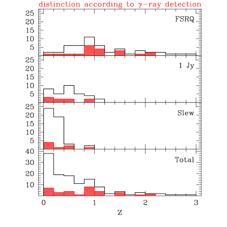
Figure 1: Redshift distributions for the three complete samples and the “total blazars sample”. Sources detected in the $\gamma$–rays are indicated by the grey areas.

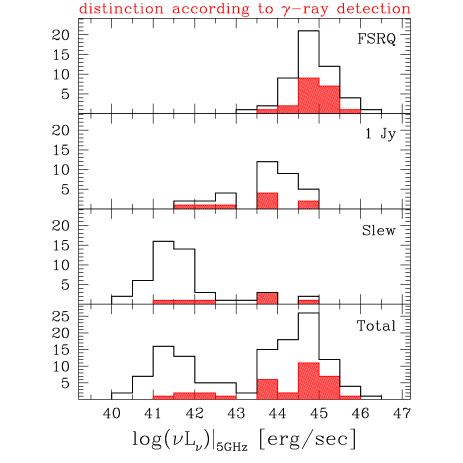
Figure 2: Distributions of L_5GHz for the three complete samples and the “total blazars sample”. Grey areas indicate $\gamma$–ray detected objects.

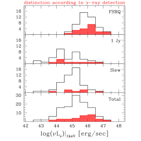
Figure 3: Distributions of L_1keV for the three complete samples and the “total blazars sample”. Grey areas indicate $\gamma$–ray detected objects.

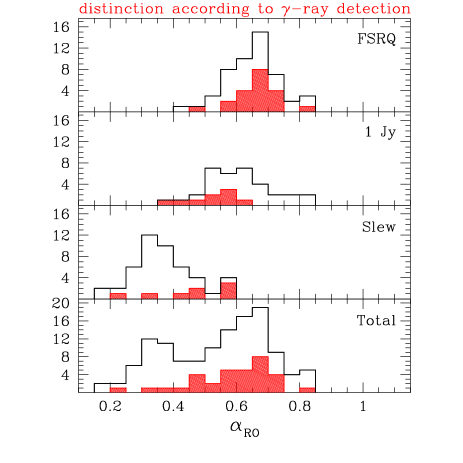
Figure 4: $\alpha_{\rm RO}$ distributions for the three complete samples and the “total blazars sample”. Grey areas indicate $\gamma$–ray detected objects.

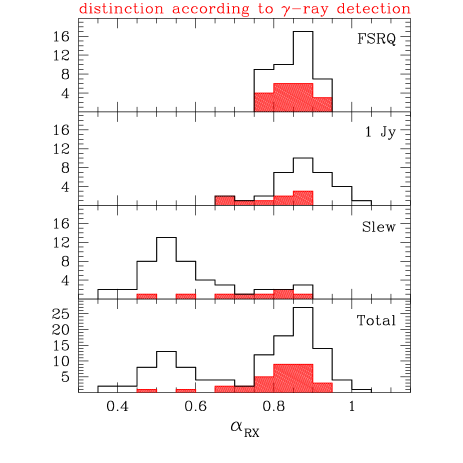
Figure 5: $\alpha_{\rm RX}$ distributions. As in Fig. 4.

The redshift distributions (Fig. 1) of the three complete samples show the known tendency towards the detection of FSRQs at higher $z$, being the latter ones more powerful radio sources, as shown in Fig. 2.

In the same figure and in Fig. 3, the tendency for XBL to have similar X–ray but lower radio luminosities compared to RBL is also apparent. Correspondingly, it appears from Figs. 4,5 that $\alpha_{\rm RO}$ and $\alpha_{\rm RX}$ increase from XBL to RBL while FSRQ have $\alpha_{\rm RO}$ slightly larger and $\alpha_{\rm RX}$ similar to RBLs. Later on (section 3.2) we will show that there is a relationship between these spectral indices and the peak frequency of the synchrotron component.

We note that for all of the distributions there is continuity in properties not only between the two BL Lac samples, but also between BL Lacs and FSRQs.

It is clear from Figs. 1-5 that for the RBL and FSRQ samples the $\gamma$–ray detected sources do not differ from non–detected ones in any of the considered quantities while for the Slew sample there is a tendency for $\gamma$–ray loud sources to have larger L_5GHz, $\alpha_{\rm RX}$ and $\alpha_{\rm RO}$. This indicates that either the radio luminosity or radio–loudness are important in determining the $\gamma$–ray detection. On the contrary, and in some sense surprisingly, the X–ray luminosity does not seem to play an important role with respect to the $\gamma$–ray emission, although the X-ray band is the closest in energy to the $\gamma$–rays . We will come back to this issue later on (§3.5). We checked the possible difference of means and variances of the distributions with the t–student’s test and only for the $\alpha_{\rm RX}$ of the Slew sample the significance is higher than 95 per cent.

Except for the case of the Slew survey, we conclude that the $\gamma$–ray detected sources are representative of the samples as a whole, being indistinguishable from the others in terms of radio to X-ray broad band properties and power.

We also checked that the $\gamma$-ray detected sources belonging to our samples are homogeneous with respect to all of the $\gamma$-ray blazars detected so far. In Fig. 6 we compare the redshift distributions, the radio luminosities and fluxes and the $\gamma$–ray spectral index. The grey shaded areas represent the $\gamma$–ray sources belonging to the complete samples considered here. We conclude that there is no significant difference.

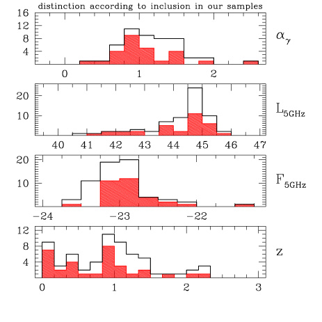
Figure 6: Distributions of redshift $z$, L_5GHz, radio flux F_5GHz and $\gamma$–ray spectral index $\alpha_{\gamma}$ for the $\gamma$–ray loud sources detected by EGRET, where the shaded ones refer only to sources in our three complete blazar samples.

Nevertheless, we are aware that the limited sensitivity of the EGRET instrument implies that at a given radio flux, only the $\gamma$–ray loudest sources are detected. Therefore the non detected ones are probably on average weaker in $\gamma$-rays. Impey (1996) quantified this effect by taking into account the correlation between radio and $\gamma$–ray luminosities (see §3.3.1), and other observables. Assuming a Gaussian distribution of the $\gamma$–ray to radio flux ratio he estimated the width of the distribution and the ”true” ratio referring to the whole population, which could be a factor 10 lower than the observed one. There could be a real spread in the intrinsic properties of the blazar population, the $\gamma$-ray detected blazars being intrinsically louder than the rest of the population. Alternatively this may be due to variability, i.e. a source is detected only when it undergoes a flare. The observed ratio would thus refer to flaring states, while the average level of each source would be lower.

Since variability is a distinctive property of blazars and has been observed to occur also in $\gamma$–rays, often with extremely large amplitude (greater than a factor 10) (e.g. 3C 279, Maraschi et al 1994; PKS 0528+134, Mukherjee et al. 1996; 1622$-$297, Mattox et al. 1997) the latter alternative is likely although the problem remains an open one. We conclude that the average $\gamma$–ray luminosities computed here are necessarily overestimated. However we chose not to correct for this effect given the uncertainties. In particular the ”bias factor” for different classes of blazars could be different if their $\gamma$–ray variability properties (amplitude and duty cycle) are (e.g. Ulrich, Maraschi & Urry 1997).

3.2 Synchrotron peak frequency

As previously noted the SEDs clearly show a broad peak between radio and UV–X–rays. In order to determine the position of the peak of the synchrotron component in individual objects with an objective procedure, we fitted the data points for each source (in a $\nu$ vs. $\nu$L_ν diagram) with a third degree polynomial, which yields a complex SED profile, with an upturn allowing for X–ray data points not to lay on the direct extrapolation from the lower energy spectrum. In many cases there is evidence that the X–ray component, even in the soft ROSAT PSPC band, is due to the inverse Compton process (e.g. Sambruna 1997; Comastri et al. 1997). Thus to impose that the X–ray point smoothly connects to the lower energy data, as would happen in a parabolic fit, could be misleading for a determination of the synchrotron peak frequency. We used a simple parabola when the cubic fit was not able to find a maximum, which typically happens when the peak occurs at energies higher than X–rays. In fact when the peak moves to high enough frequencies (typically beyond the IR band), the X–ray flux is completely dominated by the synchrotron emission, and the results given by the cubic and parabolic fits are fully consistent. In 8 cases neither the cubic nor the parabolic fit were able to determine a peak frequency/luminosity mainly due to the paucity of data points.

Figure 7: The peak frequency of the synchrotron component, $\nu_{\rm peak,sync}$, as derived with the polynomial fits, plotted against a) the radio luminosity L_5GHz, b) the $\gamma$–ray luminosity L_γ, and c) the fitted peak luminosity of the synchrotron component, L_peak,sync.

3.2.1 Synchrotron Peak Frequency vs. Luminosity

The peak frequencies derived with the above procedure (defined as the frequencies of the maximum in the fitted polynomial function) are plotted in Fig. 7a,b,c versus the radio and $\gamma$–ray luminosities and vs the corresponding peak luminosities, as determined from the fits. Let us stress once again the continuity between the different samples. Considering the samples together strong correlations are present between these quantities, in the sense of $\nu_{\rm peak,sync}$ decreasing with increasing luminosity. The results of Kendall’s $\tau$ statistical test (Table 4) show that the correlations are highly significant.

Since on one hand in flux limited samples spurious correlations can be introduced by the luminosity/redshift relation and on the other hand the correlations might be due to evolutionary effects genuinely related to redshift, we checked its role in two ways. We estimated the possible correlation of the relevant quantities with redshift directly, and performed partial correlation tests between two quantities subtracting out the common dependence on $z$ (Padovani 1992b)(see results in Table 4). In addition, in order to have an independent check on the redshift bias, we also considered the significance of the correlations restricting them to objects with $z<0.5$ (see Table 4).

The correlation between $\nu_{\rm peak,sync}$ and L_5GHz still holds after subtraction of the very strong dependence on redshift. The same is true for the relation between $\nu_{\rm peak,sync}$ and the $\gamma$-ray luminosity, although the significance is much smaller, due to the smaller number of sources. On the other hand the correlation between $\nu_{\rm peak,sync}$ and L_peak,sync is strongly weakened when subtracting the redshift effect.

Considering only the $z<0.5$ interval the significance of the first two correlations persists and does not change when the redshift dependence is subtracted. These values can then be considered as irreducible, being the signature of a true dependence of $\nu_{\rm peak,sync}$ on luminosity. This result can also be read as a check of the reliability of the partial correlation procedure. On the contrary the correlation $\nu_{\rm peak,sync}$ vs. L_peak,sync disappears at low redshifts, due to the narrow interval of values spanned by L_peak,sync, that varies less with the change of peak frequency than both radio and $\gamma$–ray luminosity do.

Table 4: Correlation probabilities according to the Kendall’s $\tau$ test. (1–2): quantities considered in the correlation; (3–10): significance of the “null–hypothesis”, i.e. that the correlation is the result of pure chance, for the various quantities: in columns (3–6) for tests performed without any redshift constraint, while in (7–10) results for tests taking into account only sources with z ${{}_{>}\atop{}^{\sim}}$ 0.5. In (3),(7) the “face value” correlation between x₁ and x₂. In (4–5) and (8–9) the significance of the correlation of each quantity x₁ and x₂ with redshift. In (6) and (10) the “net” x₁/x₂ correlation remaining from (3) and (7) after subtraction of the redshift dependence of x₁ and x₂ via partial correlation algorithm. A dash is reported the correlation is not significant (i.e. probability $<$ 90 %.

z unconstrained (# 109a)

z $<$ 0.5 (# 51a)

x1

x2

x1/x2

x1/z

x2/z

x1/x2$-Z$

x1/x2

x1/z

x2/z

x1/x2$-Z$

(1)

(2)

(3)

(4)

(5)

(6)

(7)

(8)

(9)

(10)

$\nu_{\rm peak,sync}$

L5GHz

1.2e-16

[1.1e-9]

[1.9e-31]

1.1e-11

1.3e-8

[ — ]

[4.0e-4]

9.2e-9

$\nu_{\rm peak,sync}$

Lpeak,sync

4.9e-8

[1.1e-9]

[9.5e-27]

6.5e-2

—

[ — ]

[1.2e-7]

—-

$\nu_{\rm peak,sync}$

$\alpha_{\rm RO}$

1.1e-23

[1.1e-9]

[7.7e-11]

4.7e-19

1.8e-7

[ — ]

[ — ]

2.9e-7

$\nu_{\rm peak,sync}$

$\alpha_{\rm RX}$

4.2e-17

[1.1e-9]

[6.0e-5]

1.9e-14

4.1e-15

[ — ]

[ — ]

8.4e-15

Correlations involving $\gamma$–ray data

EGRET sources included in our samples

z unconstrained (# 31)

z $<$ 0.5 (# 11)

$\nu_{\rm peak,sync}$

Lγ

2.1e-3

[3.4e-2]

[1.5e-10]

1.8e-2

2.4e-2

[ — ]

[2.4e-3]

6.4e-2

L5GHz

Lγ

6.0e-11

[5.5e-10]

[1.5e-10]

4.2e-5

3.9e-3

[5.2e-2]

[2.4e-3]

2.4e-2

$\nu_{\rm peak,sync}$

Lγ/Lpeak,sync

2.7e-5

[3.4e-2]

[1.5e-5]

2.2e-4

1.4e-3

[ — ]

[7.3e-1]

4.1e-3

$\nu_{\rm peak,sync}$

Lγ/L5500Å

2.5e-6

[3.4e-2]

[4.2e-5]

1.7e-5

2.4e-3

[ — ]

[ — ]

6.8e-3

sources in the whole EGRET sample

z unconstrained (# 60)

z $<$ 0.5 (# 15)

L5GHz

Lγ

4.8e-15

[4.8e-15]

[1.8e-14]

2.4e-6

1.8e-3

[1.1e-2]

[1.4e-4]

4.1e-2

Notes to Table 4:

^(a) we considered only sources with at least a lower limit on redshift, and for which it has been possible to determine the “synchrotron” peak frequency by means of the polynomial fit.

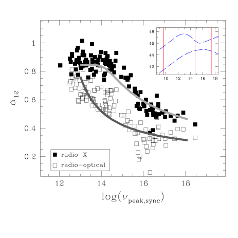
Figure 8: The broad band spectral indices $\alpha_{\rm RO}$ and $\alpha_{\rm RX}$ are plotted vs $\nu_{\rm peak,sync}$. The curved lines overlayed to the data points represent the relations $\alpha_{\rm RO}$–$\nu_{\rm peak,sync}$ and $\alpha_{\rm RX}$–$\nu_{\rm peak,sync}$ obtained from a “synthetic” set of SEDs. Details on the adopted analytical parameterization are given in text, §4. Two examples of typical SEDs are reported for reference in the inset: the top one peaking at $\nu\sim 10^{13}$ Hz, with $\alpha_{\rm RO}=0.76$ and $\alpha_{\rm RX}=0.85$, the bottom one at $\nu\sim 10^{16}$ Hz ($\alpha_{\rm RO}=0.35$ and $\alpha_{\rm RX}=0.56$). The three vertical lines mark the frequencies corresponding to 5 GHz, 5500 Å, and 1 keV, entering in the definitions of $\alpha_{\rm RO}$ and $\alpha_{\rm RX}$.

3.2.2 Synchrotron Peak Frequency vs. Broad Band Spectral indices

The relations between the synchrotron peak frequency and each of the two point spectral indices $\alpha_{\rm RO}$ and $\alpha_{\rm RX}$ are shown in Fig. 8. Also these quantities are strongly correlated (see Table 4). In fact recent papers (e.g. Maraschi et al. 1995; Comastri et al. 1995; Comastri et al. 1997), suggested that the position of the synchrotron peak could be devised from the values of broad band spectral indices.

We see that the knowledge of any of the two spectral indices is enough to guess the position of the peak of the synchrotron component, except for some ranges, namely $\nu_{\rm peak,sync}>10^{16-17}$ Hz for both $\alpha_{\rm RO}$ and $\alpha_{\rm RX}$, and $\nu_{\rm peak,sync}<10^{14}$ Hz for $\alpha_{\rm RX}$. These “failures” can be explained bearing in mind the typical shape of the blazar SEDs (see inset in Fig. 8): when the spectrum peaks at low frequencies, X–rays are typically dominated by the inverse Compton, flat spectrum, component whose luminosity level is strongly correlated with the radio one (Fossati et al. 1997), and then the X–ray/radio ratio (i.e. $\alpha_{\rm RX}$) tends to a fixed value. Conversely the Compton component begins to dominate the (ROSAT) X-ray band when $\alpha_{\rm RX}\sim 0.75$, corresponding to $\nu_{\rm peak,sync}{{}_{>}\atop{}^{{}_{<}}}3\times 10^{14}$ Hz. It is interesting to note that the adopted dividing threshold between LBL and HBL has been set to this same value from purely practical purposes, while in the light of the result above it assumes a more “physical” meaning. LBL sources have Compton–dominated soft–X–ray emission, while in HBL this is pure synchrotron.

At the other end of the spectrum a problem arises when $\nu_{\rm peak,sync}$ moves at energies higher than that used to compute the broad band spectral index. The reason is that the ratio between, for instance, optical and radio luminosity is no longer sensitive to the peak moving further towards higher frequencies, because both the radio and optical bands lay on the same (rising) branch of the synchrotron “bump”.

For comparison we draw in Fig. 8 the loci of $\alpha_{\rm RO}$–$\nu_{\rm peak,sync}$ and $\alpha_{\rm RX}$–$\nu_{\rm peak,sync}$ obtained from a set of SEDs of the kind reported in the inset, and that we are going to discuss in more detail in section 3.5. The parameterization describes the observed features very well.

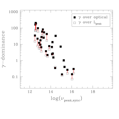
Figure 9: The $\gamma$–ray dominance (according to two definitions, see text) versus the synchrotron peak frequency $\nu_{\rm peak,sync}$

3.2.3 Synchrotron Peak Frequency vs. $\gamma$–ray dominance

In Fig. 9 $\nu_{\rm peak,sync}$ is plotted against the $\gamma$–ray dominance parameter, defined as the ratio between the $\gamma$–ray and the synchrotron peak luminosities. A strong correlation (see Table 4) is present over four orders of magnitude in $\nu_{\rm peak,sync}$, in the sense of a decrease in the $\gamma$–ray dominance with an increase of the synchrotron peak frequency. In the same figure we plotted also the ratio between the $\gamma$–ray and optical luminosities, to check if the latter could eventually be a good indicator of the $\gamma$–ray dominance, with the advantage of being an observed quantity. In fact there is little difference, at most a factor 3 for a quantity spanning more than three decades.

3.3 Average SEDS

Having discussed extensively the possible biases introduced by the limited number of $\gamma$–ray detected sources in the complete samples we construct here the average SEDs for each sample. We will come back later to the bias problem (Section 4).

The averaging procedure has been performed on the logarithms of the luminosities at each frequency. Apart from the problems in the $\gamma$-ray range discussed above the incompleteness of the data coverage at some frequencies could also introduce a bias in the average values. For instance in the Slew survey sample only 10/48 objects have a flux measured at 230 GHz, and they are the more luminous sources at 5 GHz. Averaging independently L_230GHz (for 10 objects) and L_5GHz (for 48 objects) we would obtain a ratio between the two luminosities higher than that derived considering only the subsample of 10 sources, and presumably higher than the actual one, too.

To reduce this kind of effect we first normalized the monochromatic luminosities to the radio luminosity for each source, we computed average ratios $\langle\log(L_{\nu^{*}}/L_{\rm 5GHz})\rangle|_{sub}$, considering only the subsample of sources with a measured flux at $\nu^{*}$, and used that ratio to compute the average monochromatic luminosity at $\nu*$ for all sources in the sample as $\langle\log(L_{\nu^{*}})\rangle|_{all}=\langle\log(L_{\rm 5GHz})\rangle|_{all}+\langle\log(L_{\nu^{*}}/L_{\rm 5GHz})\rangle|_{sub}$. In this way we basically averaged the spectral shape between $\nu^{*}$ and 5 GHz for the measured objects and assigned that spectral shape to the sample.

The X–ray and $\gamma$–ray spectral indices have been averaged with a simple mean, without weighting.

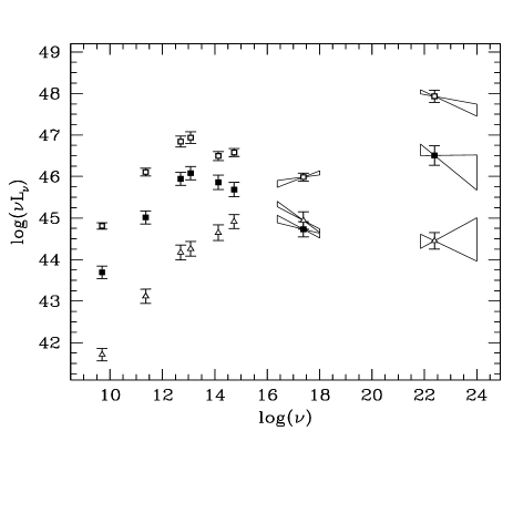
Figure 10: The average SEDs for each of the samples are shown. From top to bottom (referring to radio luminosity) Wall & Peacock FSRQs (empty boxes), 1 Jy BL Lac sample (filled boxes) and Slew survey BL Lac sample (triangles) . These latter two are in reversed order in X–ray band, the lowest spectrum being that of the 1 Jy sample.

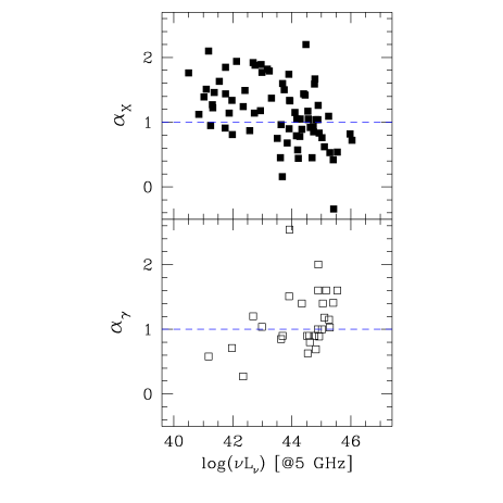
Figure 11: X–ray and $\gamma$–ray spectral indices plotted against radio luminosity.

The average broad band spectra for each of the three samples are shown in Fig. 10. The 6 sources common to the radio and the X–ray selected BL Lac samples are considered in both of them. Average luminosities entering Fig. 10 are reported in Table 5 together with the number of sources contributing at each frequency.

It is apparent from Fig. 10 that the three samples refer to objects with different average integrated luminosities and that the peak frequency of the power emitted between the radio and the X-ray band moves from the X-ray to the far infrared band going from the XBL to the FSRQ samples as anticipated from the analysis of single objects in the previous section 3.2. Correspondingly the $\gamma$–ray luminosities increase and the $\gamma$–ray spectra steepen suggesting that also the peak frequency of the high energy emission moves to lower frequencies. The overall similarity and regularity of the SEDs of the different samples as well as the continuity in the properties of the individual objects discussed in section 3.2 suggest a basic similarity of all blazars irrespective of their original classification and different appearance in a specific spectral band.

Table 5: Average luminosities, for each sample and for the total one (divided in bins of radio luminosity)

		Complete Samples				Total Blazar Sample (log(L5GHz) intervals)
	Band	Slew	1 Jy	W&P		$<$42	42$-$43	43$-$44	44$-$45	$>$45
	5 GHz	41.71	43.69	44.81		41.24	42.47	43.71	44.54	45.39
		48	34	50		38	10	17	44	17
	230 GHz	43.11	45.01	46.11		42.64	43.77	45.13	45.83	46.63
		10	34	50		5	7	15	44	17
	60 $\mu$m	44.17	45.94	46.84		43.73	44.65	46.09	46.65	47.61
		12	19	13		6	5	8	16	2
	25 $\mu$m	44.25	46.07	46.93		43.74	44.95	46.08	46.79	47.69
		10	15	8		4	6	7	9	2
	K–band	44.64	45.86	46.49		44.42	45.04	45.96	46.27	47.21
		23	31	28		13	10	15	32	6
	V–band	44.91	45.68	46.58		44.61	45.01	45.82	46.27	47.21
		48	34	50		38	10	17	44	17
	1 keV	44.94	44.72	45.98		44.81	44.11	44.92	45.66	46.50
		48	32	43		38	10	15	42	12
	100 MeV	44.45	46.50	47.93		44.24	44.79	46.67	47.71	48.68
		7	8	20		3	5	9	33	12
	$\alpha_{\rm X}$	1.40 $\pm$ 0.07	1.25 $\pm$ 0.09	0.83 $\pm$ 0.08		1.37 $\pm$ 0.09	1.55 $\pm$ 0.15	1.16$\pm$ 0.14	1.11 $\pm$ 0.08	0.57 $\pm$ 0.13
		24	31	24		16	8	14	26	9
	$\alpha_{\gamma}$	0.98 $\pm$ 0.32	1.26 $\pm$ 0.26	1.21 $\pm$ 0.09		0.64 $\pm$ 0.07	0.73 $\pm$ 0.47	1.37 $\pm$ 0.31	1.06 $\pm$ 0.13	1.30 $\pm$ 0.08
		6	6	18		2	4	7	25	11

References to Table 5:

(5 and 230 GHz): Becker, White & Edwards 1991; Bloom et al. 1994; Gear et al. 1986; Gear 1993a; Gear et al. 1994; Kühr et al. 1981; Kühr & Schmidt 1990; Perlman et al. 1996a; Reuter et al. 1997; Steppe et al. 1988, 1992, 1993; Stevens et al. 1994; Stickel et al. 1991; Stickel et al. 1993; Stickel, Meisenheimer & Kühr 1994;Tornikovski et al. 1993, 1996; Terasranta et al. 1992.

(IR–optical data): Allen, Ward & Hyland 1982; Ballard et al. 1990; Bersanelli et al. 1992; Bloom et al. 1994; Brindle et al. 1986; Brown et al. 1989; Elvis et al. 1994; Falomo et al. 1988; Falomo et al. 1993a; Falomo et al. 1993b; Falomo, Scarpa & Bersanelli 1994; Gear et al. 1986; Gear 1993b; Glass 1979, 1981; Holmes et al. 1984; Impey & Brand 1981; Impey & Brand 1982; Impey et al. 1982; Impey et al. 1984; Impey & Neugebauer 1988; Impey & Tapia 1988, 1990; Jannuzi, Smith & Elston 1993, 1994; Landau et al. 1986; Lepine, Braz & Epchtein 1985; Lichtfield et al. 1994; Lorenzetti et al. 1990; Mead et al. 1990; O’Dell et al. 1978; Pian et al. 1994; Sitko & Sitko 1991; Smith et al. 1987; Stevens et al. 1994; Wright, Ables & Allen 1983.

(X–rays): Brinkmann et al. 1994; Brinkmann et al. 1995; Brunner et al. 1994; Comastri et al 1995; Comastri et al 1997; Lamer, Brunner & Staubert 1996; Maraschi et al. 1995; Perlman et al. 1996a; Perlman et al. 1996b; Sambruna 1997; Urry et al. 1996.

($\gamma$–rays): Bertsch et al. 1993; Catanese et al. 1997; Chiang et al. 1995; Dingus et al. 1996; Fichtel et al. 1994; Hartman et al. 1993; Lin et al. 1995; Lin et al. 1996; Madejski et al. 1996; Mattox et al. 1997; Mukherjee et al. 1995, 1996; Nolan et al. 1996; Quinn et al. 1996; Radecke et al. 1995; Shrader et al. 1996; Sreekumar et al. 1996; Thompson et al. 1993; Thompson et al. 1995; Thompson et al. 1996; Vestrand, Stacy & Sreekumar 1995; von Montigny et al. 1995.

We therefore considered the merged total sample with the scope of finding the key parameter(s) governing the whole blazar phenomenology. Since luminosity appears to have an important role in that it correlates with the main spectral parameters we decided to bin the total blazar sample according to luminosity, irrespective of the original classification. We used the 5 GHz radio luminosity which is available for all objects. It may be desirable to use the total integrated luminosity which in all cases is close to the $\gamma$–ray one. However the latter is only available for a few objects. We note that a correlation between $\gamma$–ray and radio luminosity has been claimed by many authors using different techniques (Dondi & Ghisellini, 1995; Mattox et al. 1997). It is however still being debated whether it is true or it arises from selection effects, connected with the common redshift dependence of luminosities, and with the exclusion of upper limits, which could favour the appearance of a spurious correlation. It is worth mentioning that Mücke et al. (1997) using a technique designed to take into account both these effects did not find any significant correlation between radio and $\gamma$-ray data for a sample of 38 extragalactic EGRET sources.

We also checked this correlation on both the 31 EGRET detected sources included in our samples and the larger “comparison sample” of 62 EGRET sources. In Table 4 we report the significance of the correlation, together with its value after subtracting the common redshift dependence through a partial correlation test, and its significance for samples restricted to $z<0.5$. In all cases the radio and $\gamma$–ray luminosities correlate significantly.

In Figs. 11 $\alpha_{\rm X}$ and $\alpha_{\gamma}$ for individual sources are plotted against the radio power, both showing a good correlation with it. Comastri et al. (1997) discussed the interesting consequences of the apparent anti–correlation between X–ray and $\gamma$-ray spectral indices, without relating it to any “absolute” parameter, such as luminosity. Here again we see that these other spectral properties have a dependence on radio luminosity.

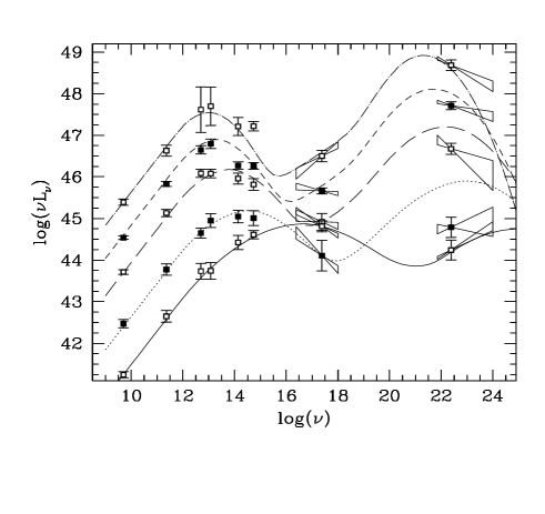
Figure 12: Average SEDs for the “total blazar sample” binned according to radio luminosity irrespective of the original classification. The overlayed curves are analytic approximations obtained according to the one–parameter–family definition described in the text.

Since in some luminosity bins the number of $\gamma$-ray detected sources is small, we used an indirect procedure to associate $\gamma$–ray fluxes and spectra to our average SEDs, taking advantage of the whole body of information regarding the $\gamma$–ray properties of blazars. Namely for each luminosity bin $\langle$L${}_{\gamma}\rangle$ and $\langle\alpha_{\gamma}\rangle$ were computed from blazars in the general EGRET–detected sample falling into the same L_5GHz bin. The basic assumption is the uniformity of the spectral properties, as discussed in section 3.1. The resulting SEDs are shown in Fig. 12 and average luminosities, X–ray and $\gamma$–ray spectral indices, and number of sources are reported in Table 5. The most interesting result is that the trends pointed out for the three separate sub–classes of blazars (Fig. 10) hold for the total blazar sample, irrespective of the original classification of sources, when the radio luminosity is adopted as the key parameter characterizing each object.

4 Discussion

In Fig. 12 we superimposed to the averaged data a set of (dashed) lines, whose main goal is to guide the eye. The radio–X–ray SED is approximated with a power law starting in the radio domain continuously connecting at $\nu\simeq 5\times 10^{11}$ Hz with a parabolic branch. This latter describes the peak of the SED and its steepening beyond it. In soft X–rays a rising power law, representing the onset of the hard inverse Compton component is summed to this curved “synchrotron” component. The normalization of this second X–ray component is kept fixed relative to the radio one. Based on our findings (see Fig. 7a), we then assume that the peak frequency of the synchrotron spectral component is (inversely) related to radio luminosity. The simplest hypothesis of a straight unique relationship between $\nu_{\rm peak,sync}$ and L_5GHz does not give a good result when compared with the average SEDs. We then allow for a different SED–shape/luminosity dependence for high and low luminosity objects, a distinction that turns out to roughly correspond also to that between objects with and without prominent emission lines. We adopted a “two–branch” relationship between $\nu_{\rm peak,sync}$ and L_5GHz in the form of two power laws $\nu_{\rm peak,sync}\propto$ L${}_{\rm 5GHz}^{-\eta}$, with $\eta=0.6$ or $\eta=1.8$ for log(L_5GHz) higher or smaller than 42.5, respectively. The shape of the analytic SEDs is parabolic with a smooth connection to a fixed power law in the radio and the loci of the maxima as defined above. A full description of the parameterization can be found in Fossati et al. (1997) where a similar scheme was proposed to account for the source number densities of BL Lacs with different spectral properties (LBL and HBL).

The analytic representation of the second spectral component (X–ray to $\gamma$–rays) is a parabola of the same width as the synchrotron one, and has been obtained assuming that: (a) the ratio of the frequencies of the high and low energy peaks is constant ($\nu_{\rm peak,Compt}/\nu_{\rm peak,sync}~{}\simeq 5\times 10^{8}$), (b) the high energy ($\gamma$–ray) peak and radio luminosities have a fixed ratio, $\nu_{\gamma}$L${}_{\rm peak,gamma}/\nu_{\rm 5GHz}$L${}_{\rm 5GHz}\simeq 3\times 10^{3}$. Given the extreme simplicity of the latter assumptions, it is remarkable that the phenomenological analytic model describes the run of the average SEDs reasonably well. The worst case refers to the second luminosity bin: the analytic model predicts a $\gamma$-ray luminosity larger than the computed bin average by a factor of 10 (but predicts the correct spectral shape). We note that only 5 $\gamma$–ray detected objects fall in this bin.

The results derived from the above analysis (see in particular Figs. 10–12) can then be summarized as follows:

1. two peaks are present in all the SEDs. The first one (synchrotron) is anticorrelated with the source luminosity (see Figs. 7 and Table 4), moving from $\sim 10^{16}-10^{17}$ Hz for less luminous sources to $\sim 10^{13}-10^{14}$ Hz for the most luminous ones.

2. the X–ray spectrum becomes harder while the $\gamma$–ray spectrum softens with increasing luminosity, indicating that the second (Compton) peak of the SEDs also moves to lower frequencies from $\sim 10^{24}-10^{25}$ Hz for less luminous sources to $\sim 10^{21}-10^{22}$ Hz for the most luminous ones;

3. therefore the frequencies of the two peaks are correlated: the smaller the $\nu_{\rm peak,sync}$ the smaller the peak frequency of the high energy component; a comparison with the analytic curves shows that the data are consistent with a constant ratio between the two peak frequencies;

4. increasing L_5GHz increases the $\gamma$–ray dominance, i.e. the ratio of the power emitted in the inverse Compton and synchrotron components, estimated with the ratio of their respective peak luminosities (see also Fig. 9).

The fact that the trends present when comparing the different samples (e.g. Fig. 10), persist when the total blazar sample is considered and binned according to radio luminosity only, suggests that we deal with a continuous spectral sequence within the blazar family, rather than with separate spectral classes. In particular the ”continuity” clearly applies also to the HBL – LBL subgroups: HBL have the lowest luminosities and the highest peak frequencies.

An interesting result apparent from the average SEDs is the variety and complexity of behaviour shown in the X–ray band. As expected the crossing between the synchrotron and inverse Compton components can occur below or above the X-ray band affecting the relation between the X–ray luminosity and that in other bands. A source can be brighter than another at 1 keV being dimmer in the rest of the radio–$\gamma$–ray spectrum except probably in the TeV range. This effect narrows the range of values spanned by L_1keV and explains why $\gamma$–ray detected sources do not select a particular range in the X–ray luminosity distributions (see Fig. 3) while this happens for L_5GHz.

Using this simple scheme of SED parameterization we can compute the luminosities in the EGRET (30 MeV – 3 GeV) and Whipple (0.3 – 10 TeV) bands. These are plotted in Fig. 13 (bottom panel) together with their ratio with the radio and X–ray luminosities (top and middle panel respectively).

It is easy to recognize that for a given radio flux sources with $\nu_{\rm peak,sync}$ around $10^{14}$ have the largest relative flux in the EGRET band, because the peak of the Compton component falls right there (Fig. 13, top panel). For higher values of $\nu_{\rm peak,sync}$ the $\gamma$–ray peak moves to higher energies too and the contribution in the EGRET band is reduced. For sufficiently high $\nu_{\rm peak,sync}$ the $\gamma$–ray peak reaches the TeV band where it becomes detectable.

Qualitatively the same general behaviour is present also in the ratios between EGRET/Whipple fluxes and the X–ray one (Fig. 13, middle panel). There are however a couple of significant differences: firstly the EGRET/X–ray ratio profile, while still peaking around $10^{14}$ Hz, is sharper than in the EGRET/radio case, secondly the TeV relative flux distribution is broader and skewed towards lower values of the synchrotron peak frequency. Thus, for a given X–ray flux (as would be the case in a flux limited X–ray selected sample) only those sources falling in the restricted interval $\nu_{\rm peak,sync}\sim 10^{13}-10^{15}$ Hz would have a flux in the EGRET band high enough to be detectable. On the other hand, for the TeV band it turns out that the chance of being observable is not confined to very extreme HBLs, with X-ray synchrotron peaks, but also intermediate BL Lacs could reach a comparable TeV flux.

Since $\nu_{\rm peak,sync}$ is directly related to both $\alpha_{\rm RO}$ and $\alpha_{\rm RX}$ we can understand now the tendency (section 3.1) of $\gamma$–ray detected sources in the Slew survey to have larger values of $\alpha_{\rm RO}$ and $\alpha_{\rm RX}$. Moreover, due to the fact that in the Slew sample LBLs are only a small fraction, the discussion above explains also the lower EGRET detection rate with respect to other blazar samples.

Figure 13: The predicted relations with $\nu_{\rm peak,sync}$ of the following quantities: the ratio of the EGRET (dashed line) and Whipple (solid line) fluxes (luminosities) with the radio one (top panel); the ratio of the EGRET and Whipple fluxes (luminosities) with the X–ray one (middle panel); EGRET and Whipple absolute luminosities (bottom panel). The $\gamma$–ray luminosities are integrated in a band approximately corresponding to that of EGRET or Whipple telescopes, 30 MeV–3 GeV and 0.3–10 TeV, respectively.

The proposed scenario relates the shape of the continuum to the total source power. It follows that predictions of this unifying scheme on both the detectability of blazars at $\gamma$–ray energies (in view of more sensitive $\gamma$–ray detectors, e.g. GLAST, improved Cherenkov telescopes, etc.), and their contribution to the $\gamma$–ray diffuse background depend on the combined effects of the SED shape, the luminosity functions and possibly evolution (Fossati et al., in preparation; see also Stecker, de Jager & Salamon 1996). In particular, an interesting and testable prediction of the scheme is the absence of high luminosity sources with synchrotron peaks in the X-ray range and strong associated TeV emission.

4.1 Interpretation

The extreme ”regularity” of the SEDs of blazars and in particular the trends discussed above must derive from the common underlying physical processes. The common scenario envisaged is that of a relativistic jet pointing close to the line of sight. Assuming the simple case of a single (homogeneous) zone model the shape of the SED depends on the spectrum of the high energy electrons radiating via synchrotron and inverse Compton, the magnetic field and the nature of seed photons for the inverse Compton process. The latter could be the synchrotron photons themselves (synchrotron self Compton, SSC) or photons outside the jet (“external Compton” EC). In the following we discuss qualitatively the implications of the suggested trends for the two scenarios.

Let us assume a constant bulk Lorentz factors in all blazars. Should the (homogeneous) SSC model be valid for all sources, it is easy to see that the (approximately) constant ratio between the high and low peak frequencies yields an (approximately) constant value for the energy of the particles radiating at the peaks (e.g. Ghisellini, Maraschi, Dondi 1996). If the energy of the radiating particles is similar in all sources the different peak frequencies should result from a systematic variation in magnetic field strength, HBLs having the highest, FSRQs the lowest random field intensity.

Should instead the soft photons upscattered to the $\gamma$–ray range be produced outside the jet at a ”typical” frequency (the same for all sources) the condition of a constant ratio between the peak frequencies implies a constant value of the magnetic field (Ghisellini, Maraschi, Dondi 1996). As a consequence the energy of the particles radiating at the peaks should vary along the spectral sequence being lower in FSRQs and higher in HBLs.

It could also be that there is a smooth transition between the SSC and EC mechanisms depending on the physical conditions outside the jet. In all cases however the role of the luminosity, which phenomenologically appears dominant, does not find an immediate physical justification, although one could find plausible arguments to link it to the parameters mentioned above and in particular to the conditions surrounding the jet.

In a separate paper (Ghisellini et al. 1998), we perform model fits to the spectral energy distributions of 51 individual objects, deriving the (model dependent) physical parameters for each source. These computations indeed suggest the idea that the blazar sequence follows from a transition from the SSC to the EC scenario, RBLs being the intermediate objects. The computed radiation energy densities, which determine the amount of radiative cooling, increase with increasing source luminosity and may be responsible for the lower energy of the particles radiating at the peaks in higher luminosity sources.

The likely possibility that the external photon field involved in the EC process is (or is related to) the radiation reprocessed as broad emission lines, seems to be at least qualitatively in agreement with the observational evidence concerning the emission line luminosity in the suggested blazar sequence.

5 Conclusions

The main conclusion of this work is that despite the differences in the continuum shapes of different sub–classes of blazars, a unitary scheme is possible, whereby Blazar continua can be described by a family of analytic curves with the source luminosity as the fundamental parameter. The ”scheme” (admittedly empirical) determines both the frequency and luminosity of the peaks in the synchrotron and inverse Compton power distributions (and therefore also the $\gamma$–ray luminosity in the EGRET range) starting from the radio luminosity only. The main suggested trend is that with increasing luminosity both the synchrotron peak and the inverse Compton peak move to lower frequencies and that the latter becomes energetically more dominant. The scheme is testable, for instance it predicts that sources emitting strongly in the TeV band have relatively low intrinsic luminosity.

The ”spectral sequence” finds a plausible interpretation in the framework of relativistic jet models radiating via the synchrotron and inverse Compton processes if the physical parameters (magnetic field and/or critical energy of the radiating electrons) vary with luminosity or if photons outside the jet become increasingly important as seed photons for the inverse Compton process in sources of larger luminosity. The latter alternative is supported at least qualitatively by the increasing dominance of emission lines in higher luminosity objects.

The proposed scenario, in which the intrinsic jet power regulates, in a continuous sequence, the observational properties from the weaker HBL, through LBL, to the most powerful FSRQs, also fits in very nicely with the unification of FR I and FR II type radio galaxies as proposed by Bicknell (1995). After a long debate the prevailing view is that FR I and FR II radio galaxies both contain relativistic jets which can be decelerated giving rise to the FR I morphology depending on the kinetic power in the jet and the pressure of the ambient medium.

The whole radio–loud AGN population could be unified in a two parameter space one being the intrinsic jet power, the other the viewing angle. An interesting point for future discussion is whether a third parameter associated with the luminosity of an accretion disk is necessary or is already implicitly and uniquely linked to the jet power.

References

Adam G., 1985, A&AS, 1985, 61, 225

Allen D.A., Ward M.J., Hyland A.R., 1982, MNRAS, 199, 969

Angel J.R.P., Stockman H.S., 1980, ARA&A, 8, 321

Ballard K.R., Mead A.R.G., Brand P.W.J.L., Hough J.H., 1990, MNRAS, 243, 640

Becker R.L., White R.L., Edwards A.L., 1991, ApJS, 75, 1

Bersanelli, M., Bouchet P., Falomo R., Tanzi E.G., 1992, AJ, 104, 28

Bertsch D.L. et al., 1993, ApJ, 405, L21

Bicknell G.V., 1995, ApJS, 101, 29

Blandford R.D., 1993, in Friedlander M., Gehrels N., Macomb D.J., eds, Proc. CGRO AIP 280. New York, p. 533

Bloom S.D., Marscher A.P., 1993, in Friedlander M., Gehrels N., Macomb D.J., eds, Proc. CGRO AIP 280. New York, p. 578

Bloom S.D., Marscher A.P., Gear W.K., Terasranta H., Valtaoja E., Aller H.D., Aller M.F. 1994, AJ, 108, 398

Bradbury S.M. et al., 1997, A&A, 320, L5

Brindle C., Hough J.H., Bailey J.A., Axon D.J., Hyland A.R., 1986, MNRAS, 221, 739

Brinkmann W., Siebert J., Boller T., 1994, A&A, 281, 355

Brinkmann W. et al., 1995, A&AS, 109, 147

Brown L.M.J. et al., 1989, ApJ, 340, 129

Brunner H., Lamer G., Worrall D.M., Staubert R., 1994, A&A, 287, 436

Catanese M. et al., 1997, ApJ, 480, 562

Chiang J, Fichtel C.E., von Montigny C., Nolan P.L., Petrosian V.,1995, ApJ, 452, 156

Comastri A., Molendi S., Ghisellini G., 1995, MNRAS, 277, 297

Comastri A., Fossati G., Ghisellini G., Molendi S., 1997, ApJ, 480, 534

Dermer C.D., Schlickeiser R., 1993, ApJ, 416, 458

Dickey J. M., Lockman F. J., 1990, ARA&A, 28, 215

Dingus B.L. et al., 1996, ApJ, 467, 589

Dondi L., Ghisellini, G. 1995, MNRAS, 273, 583

Elvis M., Lockman F. J., Wilkes B. J. 1989, AJ, 97, 777

Elvis M., Plummer D., Schachter J., Fabbiano G., 1992, ApJS, 80, 257

Elvis M. et al., 1994, ApJS, 95, 1

Falomo R., Bersanelli M., Bouchet P., Tanzi E.G., 1993a, AJ, 106, 11

Falomo R., Treves A., Chiappetti L., Maraschi L., Pian E., Tanzi E.G., 1993b, ApJ, 402, 532L

Falomo R., Scarpa R., Bersanelli M., 1994, ApJS, 93, 125

Fegan D.J., 1996, private communication

Fichtel C.E. et al., 1994, ApJS, 94, 551

Fossati G., Celotti A., Ghisellini G., Maraschi L., 1997, MNRAS, 289, 136

Gabuzda D.C., Cawthorne T.V., Roberts D.H., Wardle J.F.C., 1992, ApJ, 338, 40

Gear W.K., 1993a, MNRAS, 264, L21

Gear W.K., 1993b, MNRAS, 264, 919

Gear W.K. et al., 1985, ApJ, 291, 511

Gear W.K. et al., 1986, ApJ, 304, 295

Gear W.K. et al., 1994, MNRAS, 267, 167

Ghisellini G., Madau P., Persic M., 1987, MNRAS, 224, 257

Ghisellini G., Madau P. 1996, MNRAS, 280, 67

Ghisellini G., Maraschi L., Dondi L., 1996, A&AS, 120, 503

Ghisellini G., Padovani P., Celotti A., Maraschi L., 1993, ApJ, 407, 65

Ghisellini G., Celotti A., Fossati G., Maraschi L., Comastri A., 1998, MNRAS, submitted

Giommi P., Padovani P., 1994, MNRAS, 268, L51

Glass I.S., 1979, MNRAS, 186, L29

Glass I.S., 1981, MNRAS, 194, 795

Hartman R.C. et al., 1993, ApJ, 407, L41

Holmes P.A., Brand P.W.J.L., Impey C.D., Williams P.M., 1984, MNRAS, 210, 961

Impey C.D. 1996, AJ, 112, 2667

Impey C.D., Brand P.W.J.L., 1981, Nature, 292, 814

Impey C.D., Brand P.W.J.L., 1982, MNRAS, 201, 849

Impey C.D., Brand P.W.J.L., Wolstencroft R.D., Williams P.M., 1982, MNRAS, 200, 19

Impey C.D., Brand P.W.J.L., Wolstencroft R.D., Williams P.M., 1984, MNRAS, 209, 245

Impey C.D., Neugebauer G., 1988, AJ, 95, 307

Impey C.D., Tapia S., 1988, ApJ, 333, 666

Impey C.D., Tapia S., 1990, ApJ, 354, 124

Jannuzi B.T., Smith P.S., Elston R., 1993, ApJS, 85, 265

Jannuzi B.T., Smith P.S., Elston R., 1994, ApJ, 428, 130

Jones T.W., O’Dell S.L., Stein W.A., 1974, ApJ, 188, 353

Kühr H., Witzel A., Pauliny–Toth I.K., Nauber U., 1981, A&A, 45, 367

Lamer G., Brunner H., Staubert R., 1996, A&A, 311, 384

Landau R. et al., 1986, ApJ, 308, 78

Lepine J.R.D., Braz M.A., Epchtein N., 1985, A&A, 149, 351

Lin Y.C. et al., 1995, ApJ, 442, 96

Lichtfield S.J., Robson E.I., Stevens J.A., 1994, MNRAS, 270, 341

Lockman F. J., Savage B. D. 1995, ApJS, 97,1

Lorenzetti D., Massaro E., Perola G.C., Spinoglio L., 1990, A&A, 235, 35

Madejski G, et al., 1996, ApJ, 459, 156

Maraschi L., Rovetti F., 1994, ApJ, 436, 79

Maraschi L., Fossati G., Tagliaferri G., Treves A., 1995, ApJ, 443, 578

Maraschi L., Ghisellini G., Celotti A., 1992, ApJ, 397, L5

Maraschi L., Ghisellini G., Tanzi E.G., Treves A., 1986, ApJ, 310, 325

Mattox J.R. et al., 1997, ApJ, 476, 692

Mattox J.R., Schachter J., Molnar L., Hartman R.C., Patnaik A.R., 1997, ApJ, 481, 95

Mead A.R.G., Ballard K.R., Brand P.W.J.L., Hough J.H., Brindle C., Bailey J.A., 1990, A&AS, 83, 183

Morris S.L., Stocke J.T., Gioia I.M., Schild R.E., Wolter A., Maccacaro T., Della Ceca R., 1991, ApJ, 380, 49

Mücke A. et al., 1997, A&A, 320, 33

Mukherjee R. et al., 1995, ApJ, 445, 189

Mukherjee R. et al., 1996, ApJ, 470, 831

Murphy E.M., Lockman F.J., Laor A., & Elvis M. 1996, ApJS, 105, 369

Nolan P.L. et al., 1993, ApJ, 414, 82

Nolan P.L. et al., 1996, ApJ, 459, 100

O’Dell S.L., Puschell J.J., Stein W.A., Warner J.W., 1978, ApJS, 38, 267

Padovani P., 1992a, MNRAS, 257, 404

Padovani P., 1992b, A&A, 256, 399

Padovani P., Giommi P., 1995, ApJ, 444, 567

Padovani P., Urry C.M., 1992, ApJ, 387, 449

Pian E., Falomo R., Scarpa R., Treves A., 1994, ApJ, 432, 547

Perlman E.S., Stocke J.T., Schachter J.F., Elvis M., Ellingson E., Urry C.M., Potter M., Impey C.D., Kolchinsky P., 1996a, ApJS, 104, 251 (SLEW)

Perlman E.S., Stocke J.T., Wang Q.D., Morris S.L., 1996b, ApJ, 456, 451 (EMSS)

Quinn J. et al., 1996, ApJ, 456, L83

Radecke H.–D. et al., 1995, ApJ, 438, 659

Reuter H.-P. et al., 1997, A&AS, 122, 271

Riecke G.H., Lebofski M.J., 1985, ApJ 288, 618

Sambruna R.M., 1997, ApJ, 487, 536

Sambruna R.M., Maraschi L., Urry C.M., 1996, ApJ, 463, 444

Scarpa , Falomo R., 1997, A&A, 325, 109

Shrader C.R., Hartman R.C., Webb J.R., 1996, A&AS, 120, 599

Sikora M., Begelman M.C., Rees M.J., 1994, ApJ, 421, 153

Sitko M.L., Schmidt G.D., Stein W.A., 1985, ApJS, 59, 323

Sitko M.L., Sitko A.K., 1991, PASP, 103, 160

Smith P., Balonek T.J., Elston R., Heckert P.A., 1987, ApJS, 64, 459

Sreekumar P. et al., 1996, ApJ, 464, 628

Stecker F.W., de Jager O.C., Salamon M.H., 1996, ApJ, 473, L75

Steppe H. et al., 1988, A&AS, 75, 317

Steppe H. et al., 1992, A&AS, 96, 441

Steppe H. et al., 1993, A&AS, 102, 611

Stevens J.A. et al 1994, ApJ, 437, 91

Stickel M. et al., 1991, ApJ, 374, 431

Stickel M., Meisenheimer, K., Kühr H. 1994, A&AS, 105, 211

Terasranta H. et al., 1992, A&AS, 94, 121

Thompson D.J. et al., 1993, ApJ, 415, L13

Thompson D.J. et al., 1995, ApJS, 101, 259

Thompson D.J. et al., 1996, ApJS, 107, 227

Tornikovski M. et al., 1993, AJ, 105, 1680

Tornikovski M. et al., 1996, A&AS, 116, 157

Ulrich M.–H., Maraschi L., Urry C.M., 1997, ARA&A, 35

Urry C.M., Padovani P., 1995, PASP, 107, 803

Urry C.M., Sambruna R.M., Worrall D.M., Kollgaard R.I., Feigelson E.D., Perlman E.S., Stocke J.T., 1996, ApJ, 463, 424

Vestrand, W.T., Stacy J.G., Sreekumar P., 1995, ApJ, 454, L93

von Montigny C. et al., 1995, ApJ, 440, 525

Wall J.V., Peacock J.A., 1985, MNRAS, 216, 173

Weekes T.C. et al., 1996, A&AS, 120, 603

Wolter A., Caccianiga A., Della Ceca R., Maccacaro T., 1994, ApJ, 433, 29

Worrall D.M., Wilkes B.J., 1990, ApJ, 360, 396

Wright A., Ables J.G., Allen D.A., 1983, MNRAS, 205, 793