The Stability of Perfect Elliptic Disks.
II. A Minimal Streaming Case

Abstract

Two dimensional realizations of self-consistent models for the “perfect elliptic disks” were tested for global stability by gravitational N-body integration. The family of perfect elliptic disk potentials have two isolating integrals; time independent distribution functions $f(E,I_{2})$ which self-consistently reproduce the density distribution can be found numerically, using a modified marching scheme to compute the relative contributions of each member in a library of orbits. The possible solutions are not unique: for a given ellipticity, the models can have a range of angular momenta. Here results are presented for cases with minimal angular momentum, hence maximal random motion. As in previous work, N-body realizations were constructed using a modified quiet start technique to place particles on these orbits uniformly in action-angle space, making the initial conditions as smooth as possible. The most elliptical models initially showed bending instabilities; by the end of the run they had become slightly rounder. The most nearly axisymmetric models tended to become more elongated, reminiscent of the radial orbit instability in spherical systems. Between these extremes, there is a range of axial ratios $0.305\lesssim b/a\lesssim 0.570$ for which the minimum streaming models appear to be stable.

1 Introduction

Recent studies of elliptical galaxies and of bulges of spiral galaxies indicate that their figures are likely to be at least slightly triaxial (for reviews see Binney (1982); de Zeeuw & Franx (1991); Bertin & Stiavelli (1993)). Most elliptical galaxies appear to be supported at least in part by anisotropies in the velocity distributions rather than by rapid rotation: see, for example, the work on the dwarf elliptical galaxies NGC 147, 185 and 205 by Bender, Paquet & Nieto (1991) and Held et al. (1992). A class of non-rotating potentials, known as the perfect ellipsoids, has been advanced as a possible model for elliptical galaxies (e.g. de Zeeuw (1985)). In these potentials, the mass density is stratified on concentric, similar ellipsoids, and is non-singular in the center. Many of the properties of these potentials can be derived analytically; the orbits all have three isolating integrals, and hence properties such as the time-averaged density distribution can be computed exactly. This simplifies the task of finding self-consistent models: time-steady phase-space distribution functions $f({\bf x},{\bf v})$ such that the resulting mass density generates the desired gravitational potential. Statler (1987) and Teuben (1987) have demonstrated that distribution functions for the perfect ellipsoids, and the analogous two-dimensional elliptic disks, can be constructed. Various sub-families of the axisymmetric perfect ellipsoids have been tested for stability (de Zeeuw & Schwarzschild (1989); Merritt & Stiavelli (1990); Merritt & Hernquist (1991); Robijn & de Zeeuw (1991)).

Flattened perfect ellipsoids could also be viewed as models for galactic bars. The only analytical bar models are Freeman’s (1966a , b , c ) bars, which are based upon a rotating two dimensional harmonic oscillator potential, and the perfect elliptic disk models, which have no figure rotation. Tremaine & de Zeeuw (1987) showed that in the limit of the needle ($b\rightarrow 0$) the two dimensional perfect elliptic disk is neutrally stable. Prompted by the large streaming velocities seen in barred spiral galaxies, the stability of perfect elliptic disks with maximum angular momentum has already been studied (Levine & Sparke 1994, LS ). The roundest disks were unstable to spiral mode formation, the most elongated elliptical models were unstable to bending modes, while the models with axial ratio $b/a$ in the range $0.250\lesssim b/a\lesssim 0.570$ appeared stable. This paper extends that previous work to the study of a set of low angular momentum perfect elliptical disks. The minimal angular momentum cases allow us to study the ability of internal velocity dispersion to support an elliptic figure, and forms a natural complement to the earlier work as the other bound of the whole class of perfect elliptic disks. As before, we tested for global stability by constructing a discrete, self-consistent model, loading it into an $N$-body integrator and allowing it to evolve.

2 Orbits in The Perfect Elliptic Disk

Perfect elliptic disks are the two dimensional limiting case of the three dimensional perfect ellipsoids; their surface density $\Sigma$, derived from the perfect ellipsoid by integrating in $z$ (see Evans & de Zeeuw (1992)), is given in Cartesian coordinates $(x,y)$ by

$$\Sigma(x,y)={{\Sigma_{0}}\over{(1+{m}^{2})^{3/2}}}~{},~{}~{}~{}{m}^{2}\equiv{{x^{2}}\over{a^{2}}}+{{y^{2}}\over{b^{2}}}~{};$$ (1)

$b<a$, so that $x$ is the major axis and $y$ is the minor axis. The elliptic disk potential satisfies Stäckel’s criteria, implying that there are two integrals of motion ($E$ and $I_{2}$) and that the equations of motion are completely separable in confocal ellipsoidal coordinates (Lynden-Bell (1962); de Zeeuw (1985)). The coordinates $(\lambda,\mu)$ are the solutions to the quadratic equation

$${{x^{2}}\over{\tau+\alpha}}+{{y^{2}}\over{\tau+\beta}}=1~{},~{}~{}\alpha<\beta<0~{},$$ (2)

where for the disk of equation (1) $-\alpha=a^{2}$, $-\beta=b^{2}$. Curves of constant $\lambda$ are confocal ellipses aligned along the minor axis, with $-\alpha\leq\lambda\leq\infty$, while curves of constant $\mu$ are hyperbolae, with $-\beta\leq\mu\leq-\alpha$ (see fig. 1). All the curves share the foci $x=0,~{}y=\pm\sqrt{\beta-\alpha}$. When $\lambda\approx-\alpha$, the curves of constant $\lambda$ are highly elongated in the $y$ direction; at large $\lambda$, they become almost circular; $\lambda+\alpha\approx r^{2}$. The curve $\mu=-\beta$ lies along the $x$-axis; as $\mu$ increases, the hyperbolae bend more sharply around the foci.

The orbits in the elliptic disk potential divide into two families, box and loop orbits. The box orbits resemble Lissajous figures, combinations of independent oscillations in the $x$ and $y$ directions; they have no net angular momentum about the center of the potential. Loop orbits are ellipses or rosettes with a definite sense of rotation about the center of the potential. Because of the separability of the potential, the orbital bounding surfaces (extrema of $\lambda$ and $\mu$) or turning points of the orbit are all lines of constant $\lambda$ or $\mu$. Loop orbits are bounded by ellipses of constant $\lambda$, given by the inner and outer turning points $\lambda_{1}$ and $\lambda_{2}$; a closed loop orbit is a curve of constant $\lambda$. Box orbits are contained within an hyperbola of constant $\mu$ and an ellipse of constant $\lambda$, corresponding to the turning points $\mu_{1}$ and $\lambda_{2}$. Only the loop orbits cross the minor axis outside the foci; within the foci, only the box orbits do so (see fig. 1). An orbit may be characterized by its isolating integrals, by its actions, or by its turning points. A more complete discussion, and transformations between the defining pairs can be found in LS, section 2.

3 Constructing a self–consistent model

Constructing a self-consistent model of a given potential amounts to finding a set of orbits specified by the values $E_{k}$, and $I_{2k}$ of $E$ and $I_{2}$ and a distribution weighting function $w_{k}$ that together approximately reproduce the overall density distribution. The time-average densities $\Sigma_{\rm orb}$ along these individual orbits at any point $(\lambda,\mu)$ must sum to

$$\Sigma(\lambda,\mu)=\sum_{k}\Sigma_{\rm orb}(\lambda,\mu;E_{k},{I_{2}}_{k})w_{k}~{}~{}.$$ (3)

There are two general approaches to the problem; we can either select a set of orbits by choosing the $E_{k}$ and ${I_{2}}_{k}$, $k=1,\cdots,N$ and then compute the distribution function weights $w_{k}$ for each orbit, or we can choose the weights $w_{k}$, and then try to find a compatible set of orbits $E_{k}$ and ${I_{2}}_{k}$.

In the first method, the problem is substantially better constrained; if there are $n$ orbits, already chosen, then we need only find $n$ weights. In the second case, we have $n$ weights, and are trying to find $2n$ orbit specifiers. The first approach has been used (Schwarzschild (1979); Statler 1987; Teuben 1987; de Zeeuw, Hunter & Schwarzschild 1987, hereafter ZHS ) to demonstrate that solutions to the self-consistent problem do exist. If we wish to construct a discrete representation of a potential, for an $N$-body simulation, then the second method has the advantage of allowing us to insist that each orbit contain an integral number of equal mass particles. LS showed that such problems could be solved successfully using the second approach; here we show that the first method can also be adapted for this purpose. Qualitative agreement between the two methods for the maximum angular momentum case has been shown in Levine (1995).

Along the minor axis, outside of the foci, the overall mass density is comprised solely of loop orbits; this provides a constraint that depends only on the selection of loop orbits. Loop orbits are also the only orbits with net angular momentum. This allows us to split the problem of choosing a set of orbits into two smaller problems. First, we select a set of loop orbits which add up to give the correct density in this region and also meet some additional criterion on the total angular momentum, and then we find a set of box orbits which contribute the rest of the mass needed.

3.1 Loop Orbit Selection

If the outer turning point $(\lambda_{2})$ of a loop orbit is fixed, then as we move the inner turning point $(\lambda_{1})$ outwards, the angular momentum of the orbit increases from a limit of zero for the marginal orbits ($\lambda_{1}=-\alpha$) up to a maximum which is reached at the closed loop orbit $\lambda_{1}=\lambda_{2}$. Similarly, for a fixed value of $\lambda_{1}$, the angular momentum of the orbit increases as we increase the value of $\lambda_{2}$. So, for maximum angular momentum, we choose the thinnest possible orbits ($\lambda_{1}=\lambda_{2}$), and for the minimal angular momentum, the thickest possible ($\lambda_{1}\ll\lambda_{2}$).

In the maximum angular momentum case, the loop orbit population is easily and uniquely determined (ZHS; LS). The closed loops can never overlap each other, so at any point on the minor axis outside the foci, one and only one closed loop orbit contributes to the density at that point; finding the mass on each of the loop orbits is a one dimensional problem. In LS, we chose a set of $n$ equally weighted orbits by integrating out from the minor axis; when the total integrated loop mass reached $1/n$ of the total loop orbit mass, we placed a single closed orbit on the mass weighted center ellipse of the elliptic annulus thus defined. The outer bound of the first orbit became the inner bound of the region represented by the next orbit, and the process was repeated until $n$ orbits had been selected.

Any other model must contain some thick loops, and very likely some of them will overlap each other, as well as the box orbits; finding a satisfactory set of loop orbits has become a two dimensional problem. We begin by dividing the minor axis into $N$ one dimensional cells, the inner-most cell boundary being the focal point ($\lambda=-\alpha$), and the outer-most being the outer limit in $\lambda$ $(\lambda_{\rm out})$. We create a library of $N(N+1)/2$ orbits whose inner and outer turning points lie on the boundaries of the cells $(\lambda_{\rm cd})$. For each outer turning point at $\lambda_{\rm cd}(i=k)~{}(k=1,\cdots,N)$ there are $k$ inner turning points from $\lambda_{\rm cd}(i=0)$ (close to the marginal orbit) out to $\lambda_{\rm cd}(i=k-1)$ (close to the closed loop orbit). From this library, we choose at most $N$ orbits having non-zero weight, and compute weights $w_{\rm cd}$ for each member of the set of loop orbits. Because we must match the density in $N$ cells, and have $N(N+1)/2$ possible orbits, the problem is under-constrained. The maximal and minimal angular momentum solutions are two cases where an angular momentum criterion coupled with the density matching restricts the possible solutions to a unique solution for a given library of orbits.

To find a minimal angular momentum solution, we compute the weights sequentially, starting with the loops with their outer turning point in the outer-most cell. We take the loop closest to the marginal orbit (the “thickest” loop), and choose its weight so that it accounts for all of the mass in that cell. This fills the outermost cell with material from the orbit of lowest angular momentum which reachs that cell. The mass which must still be placed in all the inner cells is then reduced by subtracting off the contribution of this orbit, while making sure that the density left in each cell is non-negative. If this is so, we move to the next outer-most cell, and repeat the process, and so step our way in towards the center. As we near the center, the contributions of the low angular momentum loops to the inner cells may fill some of them completely, before filling the outer-most loop. When this happens, we reduce the weight of the outermost orbit so that the remaining mass in each cell is non-negative, and then move the inner turning point out by one cell, and continue the process. We found that the loop orbit portion of the self-consistent model cannot be made up solely of marginal orbits; it is not possible to construct a model with exactly zero angular momentum.

We have not proven formally that we have the minimum angular momentum case, but empirically we appear to be close to the minumum; the angular momenta of these models are $\sim 10^{-3}$ times less than that of the maximum streaming models. As a check, we tried breaking up the solution space into an inner and an outer region at a $\lambda$ cell boundary, and solving first the outer and then the inner regions separately and adding up the solutions; no matter what boundary was chosen, the angular momentum was greater than in the original single region solution. In addition, the derivative of the angular momentum with respect to the inner turning point is quite steep, implying that we really want to push towards most marginal, as we have done.

If the integrated linear density in the cells varies too greatly, we may not be able to find a positive solution. We separated the cell boundaries by uniform increments in their square roots, so that the cell divisions lie at

$$\lambda_{\rm cd}(i)=\left\{\sqrt{-\alpha+\delta}+(\sqrt{\lambda_{\rm out}}-\sqrt{-\alpha+\delta})\frac{i}{N}\right\}^{2}\mbox{for $i=(0,1,\cdots,N)$.}$$ (4)

(The small quantity $\delta=5\times 10^{-5}$ is added to the inner-most boundary to avoid the non-integrable singularity at $\lambda=-\alpha$.) The choice of square root spacing spreads the distribution function weights fairly evenly among the orbits. The problem can be solved with other spacings (we have used linear and exponential spacings as well though using an exponential cell spacing for the less centrally concentrated models did not always lead to a positive solution), but with much greater contrast in the orbit weights.

As the axial ratio gets smaller, the gradient of the density along the minor axis (and overall) increases, making it desirable to use more cells to achieve a better approximation of the loop orbit density. If the number of cells on the minor axis is too small, then the discrete solution does not well approximate the continuous reality. Conversely, if the number is very large, then each orbit will end up being represented by a very small number of particles, and hence will itself not be well sampled. For $b/a=0.125$, $0.570$ and $0.910$, we computed solutions using between 100 and 1200 cells. We then chose the number of cells to be as small as possible and still give a good approximation to what appeared to be the limiting continuous solution. Figures 2 and 3 show respectively the relative weights of orbits as a function of turning points and the distribution of particles for 100 and 400 orbit library solutions. We decided to use 400 cells along the minor axis for all of the models; this provided a good compromise between good sampling of the linear density, and allowing high enough weights to permit us to sample each orbit reasonably well.

3.2 Box Orbit Selection

For the box orbits, the method of solution follows the method of ZHS; it is conceptually the same as for the loops, except that the grid is a full rectangle. First, the area of the disk is divided up into a grid in the coordinates $(\lambda,\mu)$, with the grid points in both $\lambda$ and $\mu$ spaced by uniform increments in the square root (just as in the loop orbit case). For each grid cell, the coordinates of the corner with maximum $\lambda$ and $\mu$ are the turning points of the box orbits in the library. In each cell we compute the integrated surface density minus the sum of the surface densities already allocated to the loop orbits. For the box orbit with turning points in the outermost grid cell denoted $(1,1)$ in Fig. 4, the orbit’s weight is chosen so as to supply all the mass in the cell. The contribution of this orbit is then subtracted from each of the inner cells, and the process repeated for the next outermost orbit and cell (denoted $(1,2)$), working inwards until weights have been computed for all the orbits. ZHS have previously shown that positive definite solutions do exist for the maximum streaming case; our experience is that solutions also exist for these minimum streaming models.

We have chosen to use a library of orbits with 60 turning points in $\lambda$ and 30 in $\mu$, making for 1800 orbits and cells. Figure 3 shows the difference in relative sampling between a library of $20\times 20$ orbits and one with $60\times 30$ orbits once they are populated with particles.

4 Populating the Orbits

We then place particles upon each orbit in a quiet manner, so as to minimize random noise in the initial conditions, and make it easier to watch for the growth of instabilities. The quiet distribution is our best approximation to a uniform distribution of particles throughout the phase space explored by an orbit. For a closed orbit, the solution is easily found (Sellwood (1983)). For our space filling orbits in an integrable potential, we use a slightly modified version of the technique described in detail in LS. We place particles at the intersection points of a grid on the torus in action–angle space which corresponds to each orbit. To find the starting positions and velocities of each particle, we construct a differential map from action–angle space to position and velocity coordinates.

The weight of each orbit determines how many particles should be placed on the it. In all cases, we attempt to factor the integer nearest to this number into two factors $n$, $m$ as nearly equal as possible. If the nearest integer is less than 6, then we accept whatever pair of factors we compute. Otherwise, we also factor the second nearest integer, and choose the pair of factors that are most nearly equal; this helps to avoid problems when the nearest integer is prime, or has only two, very different, prime factors. We then use a grid with $n$ lines evenly spaced in the angle $\theta_{\lambda}$ and $m$ lines in $\theta_{\mu}$. The overall difference between the desired and the computed number of particles is $\lesssim 100$ for models with 50,000 particles ($\lesssim 0.2\%$ difference), and the model produces a good approximation of the overall potential.

5 Model Setup and Integration

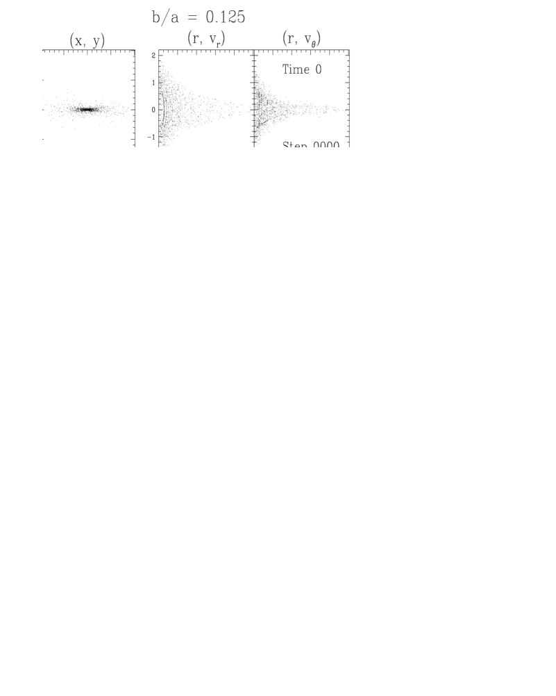
All units from here on are expressed in terms where the gravitational constant $G$, the length scale $a$, and the total mass $M_{\rm total}$ of each model when integrated analytically out to infinity are all equal to 1. Because the perfect elliptic disks are formally infinite in extent, we have truncated the models, at $r=10a$, for which all the models contain at least 90% of the total mass. Models were constructed for ellipticities ranging from $b/a=0.125$ to $0.910$ following the prescription given above. These particle distributions were then loaded into an $N$-body integrator and allowed to evolve under the influence of their own self-gravity. The fraction of the total mass within the truncation radius ($M_{\rm trunc}$), the axial ratio ($b/a$), the relative fraction of the model mass in the loop orbits, the angular momentum and the stability result for both the minimum and maximum cases of each of the models are given in Table 1.

We used a two dimensional polar-grid Fourier-transform $N$-body code developed and kindly supplied by J. Sellwood (see Sellwood (1981), 1983 and Miller (1976) for a more complete description). The grid was made up of 86 rings logarithmically spaced in radius with 100 grid points evenly spaced about them in azimuth. The grid was bounded by circles of radius $r=0.05a$ and $r=10.4a$. The outermost cells had dimensions $\Delta r=0.64a$ by $r\Delta\theta=0.66a$. Stars that crossed the outer boundary during the integration were discarded, while stars crossing into the central hole continued across it with constant velocity on a straight path, and were placed back on the grid at the next step (Sellwood (1983)). An explicit softening length of $0.05$ was used for these integrations, and a small compensating radial force correction was added to insure that our initial models were close to virial equilibrium. For an extended discussion of the details of the integration, and determination of the softening length see LS.

The integration time step $\Delta t$ was chosen to be less than $1/20^{\rm th}$ of the minimum period required for each of the angle variables to complete a circuit of $2\pi$ radians on the action–angle torus for at least 90% of the orbits. We used $\Delta t=0.01$ for all the models except $b/a=0.125$ and $0.180$, for which $\Delta t=0.002$; the most elliptic models have higher central densities and velocities, requiring better time resolution. All of the models were run for at least 20 dimensionless time units, corresponding to 3–6 crossing times at the half-mass radius. This was enough time for gross instabilities to develop. For a number of the models we continued the simulations for 100 times units (15–30 half-mass crossing times).

At the beginning of the runs, the number of particles in the central hole was less than $0.5{\rm\%}$. In the most unstable models, several hundred particles fell off the grid within $t=20$, while the stable models lost only tens of particles out of 50,000. The more elliptic models lost more particles, perhaps because of the higher radial velocities in their deeper central potentials. By $t=100$, between $2{\rm\%}$ and $14{\rm\%}$ of the particles had left the grid.

6 Results

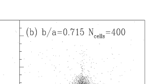
We constructed a set of minimal angular momentum models with ellipticities ranging from $0.125$ to $0.910$, highly elongated to almost circular. The minimal angular momentum models at both extremes of axial ratio appear to be unstable. For the nearly axisymmetric models (for $b/a=0.910$ to $0.640$, see fig. 5 and 6), the dominant instability manifests itself as an increase in ellipticity, resembling the radial orbit instability seen in three dimensional simulations that have little rotational support (e.g. Merritt & Aguilar (1985); Barnes, Goodman & Hut (1986)). In the most elongated models (fig. 8) where $b/a\lesssim 0.2$, we see initially the beginnings of a bending instability, just as in the maximal streaming models, and similar to the bending seen in the prolate E9 model of Merritt & Hernquist (1991). This is followed later by a decrease in the overall ellipticity of the figure, and a growth in the power in the “lopsided” $m=1$ mode similar to that seen in Palmer & Papaloizou (1990) and Palmer, Papaloizou & Allen (1990). Models with axial ratio ratio between $0.305$ and $0.570$ appear to be stable over the duration of the simulations (fig. 7).

Since the growth of an instability is not always apparent in the plots of particle position, we have also examined the behavior of the first six logarithmic spiral coefficients for these models. The growth of asymmetry in the $m=2$ mode was defined in LS eq. [31] as

$$\Delta(m=2,p)={{|A(m=2,p)|-|A(m=2,-p)|}\over{|A(m=2,p=0)|}}~{}~{};$$ (5)

this measures the spirality which is inherent in growing modes (Lynden-Bell & Ostriker (1967); LS, eq. [27] & [31]). Incipient spiral instabilities can show up here before they are clearly visible in the plots of particle positions. We call “stable” those models for which there is no change, above the noise level inherent in the particle discreteness, in the amplitude of the spiral harmonics. Figure 9 shows the change over the course of an $N$-body integration of the dominant $m=2$ log spiral mode, for the models of figures 5–8. Bending-unstable models such as $b/a=0.125$ grow asymmetrically at small $p/m$; this is most apparent as the s-shaped curve in the symmetry plot. The unstable nearly-round models which become more elliptic show a mostly symmetric growth in the $m=2$ power. Stable models such as $b/a=0.305$ don’t budge. We have labeled the models with $b/a=0.250$ and $0.640$ as marginally stable: we see global instabilities of small power develop, but these very quickly saturate and die out.

7 Discussion

In this paper and in LS, we have constructed discrete self-consistent representations of the distribution functions of a range of perfect elliptic disks with minimal and maximal angular momentum. These models were then integrated forward in time using an $N$-body integrator to see if they were stable. The nearly axisymmetric and the most elongated models were unstable. The perfect elliptic disks with moderate axial ratios appear to be stable in both the maximum and minimum streaming cases.

In the maximum streaming case, the nearly axisymmetric models developed spiral and bar instabilities as expected, since their limiting case, a cold axisymmetric disk, is known to be violently unstable to spiral instabilities. In the minimal angular momentum case, nearly-round disks became more elliptical, in a manner very similar to the radial orbit instability of spherical systems. This is not too surprising, since the velocity distribution is anisotropic, with the radial velocity dispersion being substantially higher than the tangential dispersion, even in the very nearly axisymmetric models. This comes about because of the substantial presence of box and marginal loop orbits in the models.

In both angular momentum extremes, the most elongated models developed a bending instability. The similarity in behavior is not very surprising given the decreasing importance of rotational support with increasing ellipticity in these models. Tremaine & de Zeeuw (1987) have shown that the limiting case of the needle ($b\rightarrow 0$) is neutrally stable to bending, while Merritt & Hernquist (1991) have demonstrated a bending instability in a very prolate (E9) system. It is thus not surprising that the most elliptic models should develop this instability. For the minimum angular momentum family, the instabilities change the shape of the disk towards a more moderate ellipticity.

In the nearly axisymmetric disks, as the angular momentum is decreased from a maximum, we expect that the increasing velocity dispersion should help to stabilize against spiral instabilities. It appears likely that there is a stable region for nearly axisymmetric disks with values of Toomre’s (t64 (1964)) stability parameter $Q$ which lies between the points $Q\sim 2$ and $Q\sim 3$ where the velocity dispersion has increased to the point of being able to support the disk against the spiral instability (fig 10). As the rotational support becomes negligible and the radial velocity dispersion increases, a radial–orbit instability develops; the disks with lower angular momentum become unstable to elliptical distortions when $T_{\rm radial}/T_{\rm tangential}\gtrsim 1.2$ (after the discussion of Fridman & Polyachenko (1984) and Polyachenko (1987) for stability of spherical systems). We expect that there is a range of angular momentum between the two extremes for which the nearly round disks are stable. The moderately elliptical disks with maximum and minimum angular momentum appear to be stable, so we would anticipate that disks of similar ellipticity and intermediate angular momentum will also be stable.

The stability of the two-dimensional models with moderate ellipticity gives us hope that the three dimensional perfect ellipsoids of intermediate triaxiality (which is probably the appropriate range for elliptical galaxies Mihalas & Binney (1981); de Vaucouleurs, de Vaucouleurs & Corwin (1976); de Zeeuw & Franx (1991)), will also be stable. It is known that some very flattened systems, such as the extreme oblate spheroids constructed from thin short-axis tube orbits (Merritt & Stiavelli (1990)), are unstable, but the simple fact that two longer axes are unequal is not likely to be the cause of further trouble. The three dimensional extension of this work will be interesting to see in light of the work of Allen, Palmer & Papaloizou (1992) showing that three dimensional systems with a small amount of rotational streaming are unstable to a tumbling bar instability, both when the models have largely radial orbits and when the orbits are mostly circular.

The techniques developed in this work have laid the foundation for investigating the stability of three dimensional perfect ellipsoids, and indeed of any integrable potential. The methods for choosing orbits, whether simulated annealing (as in LS) or the marching scheme of ZHS, can be easily expanded to take account of a variety of possible cost terms related to angular momentum or line of sight velocities (e.g. Rix (1997)). The procedure of LS for generating a quiet start which minimizes random noise due to particle discreteness, can be carried over to any integrable system. This is potentially most useful in $N$-body studies which attempt to measure the growth rate of instabilities, because the detection of instabilities which are still in the linear regime is limited by particle noise. For example, Saha (1991) found that his linear stability theory was consistent with the results of $N$-body simulations for highly unstable spherical systems, but predicted slow growing instabilities which could not be seen in the simulations because of particle noise. Allen, Palmer & Papaloizou (1990) have constructed an analytic potential–smoothing integration technique which decreases the $\sqrt{N}$ noise associated with binning and softening in $N$-body codes, and permits better examination of the linear growth regime. Their method would also benefit from a quiet start, because the particle discreteness then makes a larger relative contribution to the noise.

Table 1: Model Details

		Minimum $L_{z}$			Maximum $L_{z}$
$b/a$	$M_{\rm trunc}$	$\frac{M_{\rm loop}}{M_{\rm trunc}}$	${10^{3}\times L_{\rm z}}$	Stable	$\frac{M_{\rm loop}}{M_{\rm trunc}}$	${10^{3}\times L_{\rm z}}$	Stable
0.125	0.935	0.002	0.012	Bend	0.01	011.98	Bend
0.180	0.934	0.003	0.025	Bend	0.02	026.31	Bend
0.250	0.932	0.007	0.051	Marginal	0.04	050.84	Stable
0.305	0.930	0.010	0.078	Stable	0.06	076.68	Stable
0.370	0.928	0.015	0.120	Stable	0.09	114.80	Stable
0.440	0.926	0.022	0.177	Stable	0.13	165.27	Stable
0.470	0.924	0.026	0.205	Stable	0.15	189.75	Stable
0.570	0.920	0.040	0.312	Stable	0.23	284.66	Stable
0.640	0.917	0.054	0.399	Marginal	0.30	364.85	Marginal
0.715	0.914	0.074	0.497	Elliptic	0.39	463.27	Spiral
0.820	0.909	0.115	0.629	Elliptic	0.55	624.68	Spiral
0.910	0.905	0.176	0.708	Elliptic	0.73	784.92	Spiral

Figure 1: Sample loop (top) and box (bottom) orbits showing the placement of particles upon each. The orbital bounding surfaces or turning points ($\tau_{1}$ and $\tau_{2}$) are marked with dashed lines, and lines of constant angle have been plotted in the orbits to show the placement of each particle at an action–angle grid intersection. For the box orbit, the filled circles mark the intersections where particles are placed. For the loop orbit, for clarity, we have plotted only lines of constant $\theta_{\mu}$; the intersections of these with lines of $\theta_{\lambda}$ are marked with filled triangles, and squares. The open squares mark the foci of the elliptic coordinates.

Figure 2: For a model with axis ratio $b/a=0.715$, the top panel shows the turning points of the loop orbits with non-zero weight in the solution. The dashed line on the left is the line $\lambda_{1}=\lambda_{2}$. The orbits with the outermost turning points are as close to the marginal orbit as the library contains. The middle panel shows the number of particles assigned to each orbit as a function of the outer turning point ($\lambda_{2}$). The 400 loop orbits contain a total of 3760 particles. The bottom panel show the angular momentum on each orbit (solid line) and the cumulative angular momentum as a fraction of the total as a function of the orbit outer turning point (dashed line). The bulk of the angular momentum comes from the inner, non-marginal orbits.

Figure 3: For the model of figure 2, particle distributions on the loop orbits for libraries with (a) 100 and (b) 400 orbits, and on the box orbits for libraries with $N$ divisions in $\lambda$ and $M$ divisions in $\mu$, where $N\times M$ are $20\times 20$ (c) and $60\times 30$ (d) orbits respectively. The small circles seen in (a) are a result of using too few orbits, with the result that some of the loop orbits have many more particles than the rest. The solution in (a) has 1814 particles, and that in (b) has 3760.

Figure 4: The ordering of the grid cells for the box orbit library, and their respective orbits in the elliptical space in which the equations of motion separate. Nine of the outermost cells and orbits are shown explicitly, with the orbit turning points labeled by filled squares. $([x=M,\cdots,1],1)$ denote the marginal (thickest) box orbits.

         

Figure 5: Positions (left column) and velocities (radial velocity: middle column; tangential velocity: right column) for 2500 of the 50,000 particles in the $N$-body integrations are shown at times 0, 5, 10, 15 and 20, for $b/a=0.910$.

         

Figure 6: Positions (left column) and velocities (radial velocity: middle column; tangential velocity: right column) for 2500 of the 50,000 particles in the $N$-body integrations are shown at times 0, 5, 10, 15 and 20, for $b/a=0.640$.

         

Figure 7: Positions (left column) and velocities (radial velocity: middle column; tangential velocity: right column) for 2500 of the 50,000 particles in the $N$-body integrations are shown at times 0, 5, 10, 15 and 20, for $b/a=0.305$.

         

Figure 8: Positions (left column) and velocities (radial velocity: middle column; tangential velocity: right column) for 2500 of the 50,000 particles in the $N$-body integrations are shown at times 0, 5, 10, 15 and 20, for $b/a=0.125$.

         

Figure 9: The left hand column shows the distribution of power with the tangent of the pitch angle in the $m=2$ log spiral mode ($\ln|A(m=2,p)|$) for models with $b/a=$ $0.125$, $0.305$, $0.640$, and $0.910$. The right hand column shows the growth of the asymmetry term $\Delta(m=2,p)$ in the $m=2$ mode. These are plotted at times 0 (solid line), 10 (dotted line) and 20 (dashed line).

Figure 10: Disk angular momentum as a function of ellipticity for the maximum and minimal angular momentum disks. The solid line shows the angular momentum in the infinite maximum angular momentum disks, the squares the actual values in the truncated maximum angular momentum disk models, and the triangles the values for the minimal angular momentum disk models. Open and filled symbols represent unstable and stable models respectively. Values of $Q$ for axisymmetric models are indicated along the right hand axis. $T_{r}/T_{t}=0.85$ and $1.14$ for $Q=2$ and $3$ respectively.

References

- Allen, Palmer & Papaloizou (1990) Allen, A. J., Palmer, P. L., & Papaloizou, J. C. B. 1990, MNRAS, 242, 576
- Allen, Palmer & Papaloizou (1992) Allen, A. J., Palmer, P. L., & Papaloizou, J. C. B. 1992, MNRAS, 256, 695
- Barnes, Goodman & Hut (1986) Barnes, J., Goodman, J., & Hut, P. 1986, ApJ, 300, 112
- Bender, Paquet & Nieto (1991) Bender, R., Paquet, A., & Nieto, J.-L. 1991, A&A, 246,349
- Bertin & Stiavelli (1993) Bertin, G., & Stiavelli, M. 1993, Rep. Prog. Phys., 56, 493
- Binney (1982) Binney, J. 1982, ARA&A, 20, 399
- de Vaucouleurs, de Vaucouleurs & Corwin (1976) de Vaucouleurs, G., de Vaucouleurs, A., & Corwin, H. G. 1976, Second Reference Catalogue of Bright Galaxies (Austin: University of Texas Press)
- de Zeeuw (1985) de Zeeuw, P. T. 1985, MNRAS, 216, 273
- de Zeeuw & Franx (1991) de Zeeuw, P. T., & Franx, M. 1991, ARA&A, 29, 239
- (10) de Zeeuw, P. T., Hunter, C., & Schwarzschild, M. 1987, ApJ, 317, 607 (ZHS)
- de Zeeuw & Schwarzschild (1989) de Zeeuw, P. T., & Schwarzschild, M. 1989, ApJ, 345, 84
- Evans & de Zeeuw (1992) Evans, N. W., & de Zeeuw, P. T. 1992, MNRAS, 257, 152
- (13) Freeman, K. C. 1966a, MNRAS, 133, 47
- (14) Freeman, K. C. 1966b, MNRAS, 134, 1
- (15) Freeman, K. C. 1966c, MNRAS, 134, 15
- Fridman & Polyachenko (1984) Fridman, A., & Polyachenko, V. 1984, Physics of Gravitating Systems, vols. 1 and 2 (Berlin: Springer-Verlag)
- Held et al. (1992) Held, E., de Zeeuw, P. T., Mould, J., & Picard, A. 1992, AJ, 103, 851
- Levine (1995) Levine, S. E. 1995, in The Formation of the Milky Way, ed. E. J. Alfaro & A. J. Delgado (New York: Cambridge Univ. Press), 247
- (19) Levine, S. E., & Sparke, L. S. 1994, ApJ, 428, 493 (LS)
- Lynden-Bell (1962) Lynden-Bell, D. 1962, MNRAS, 124, 95
- Lynden-Bell & Ostriker (1967) Lynden-Bell, D., & Ostriker, J. P. 1967, MNRAS, 136, 239
- Merritt & Aguilar (1985) Merritt, D., & Aguilar, L. 1985, MNRAS, 217, 787
- Merritt & Hernquist (1991) Merritt, D., & Hernquist, L. 1991, ApJ, 376, 439
- Merritt & Stiavelli (1990) Merritt, D., & Stiavelli, M. 1990, ApJ, 358, 399
- Mihalas & Binney (1981) Mihalas, D., & Binney, J. 1981, Galactic Astronomy (San Francisco: W. H. Freeman)
- Miller (1976) Miller, R. H. 1976, J. Comp. Phys., 21, 400
- Palmer & Papaloizou (1990) Palmer, P. L., & Papaloizou, J. C. B. 1990, MNRAS, 243, 263
- Palmer, Papaloizou & Allen (1990) Palmer, P. L., Papaloizou, J. C. B., & Allen, A. J. 1990, MNRAS, 243, 282
- Polyachenko (1987) Polyachenko, V. 1987, in IAU Symp. 127, Structure and Dynamics of Elliptical Galaxies, ed. P. T. de Zeeuw (Dordrecht: Reidel), 301
- Rix (1997) Rix, H.-W., de Zeeuw, P. T., Cretton, N., van der Marel, R.P., Carollo, C. M. 1997, ApJ, 488, 702
- Robijn & de Zeeuw (1991) Robijn, F., & de Zeeuw, P. T. 1991, in Dynamics of Disc Galaxies, ed. B. Sundelius (Göteborg, Sweden), 373
- Saha (1991) Saha, P. 1991, MNRAS, 248, 494
- Schwarzschild (1979) Schwarzschild, M. 1979, ApJ, 232, 236
- Sellwood (1981) Sellwood, J. A. 1981, A&A, 99, 362
- Sellwood (1983) Sellwood, J. A. 1983, J. Comp. Phys., 50, 337
- Statler (1987) Statler, T. 1987, ApJ, 321 113
- Teuben (1987) Teuben, P. J. 1987, MNRAS, 227, 815
- (38) Toomre, A. 1964, ApJ, 139, 1217
- Tremaine & de Zeeuw (1987) Tremaine, S., & de Zeeuw, P. T. 1987, in IAU Symp. 127, Structure and Dynamics of Elliptic Galaxies, ed. P. T. de Zeeuw (Dordrecht: Reidel), 493