IRAS 06562$-$0337, The Iron Clad Nebula:
A New Young Star Cluster

Abstract

IRAS 06562$-$0337 has been the recent subject of a classic debate: proto-planetary nebula or young stellar object? We present the first 2$\micron$ image of IRAS 06562$-$0337, which reveals an extended diffuse nebula containing approximately 70 stars inside a 30$\arcsec$ radius around a bright, possibly resolved, central object. The derived stellar luminosity function is consistent with that expected from a single coeval population, and the brightness of the nebulosity is consistent with the predicted flux of unresolved low-mass stars. The stars and nebulosity are spatially coincident with strong CO line emission. We therefore identify IRAS 06562$-$0337 as a new young star cluster embedded in its placental molecular cloud. The central object is likely a Herbig Be star, $M\approx 20M_{\odot}$, which may be seen in reflection. We present medium resolution, high S/N, 1997 epoch optical spectra of the central object. Comparison with previously published spectra shows new evidence for time variable permitted and forbidden line emission, including Si II, Fe II, [Fe II], and [O I]. We suggest the origin is a dynamic stellar wind in the extended, stratified atmosphere of the massive central star in IRAS 06562$-$0337.

1 Introduction

Garcia-Lario, Manchado, Sahu, and Pottasch (1993, hereafter GMSP) present the first detailed analysis of IRAS 06562$-$0337. They argue that it is a proto-planetary nebula (PPN) undergoing final mass-loss episodes. Their time-series of optical spectra, obtained over a 5 year period, show the onset of forbidden line emission and the possible evolution of the central star toward hotter temperatures. They derive a Zanstra temperature of 2$\times$10⁴ K, with a slight increase over a two year interval. The effective temperature of the exciting star, T_eff $\approx$ 3.6$\times$10⁴ K, also showed a slight increase in two years. The H$\alpha$ line profile changes in time, which GMSP interpret as variable high velocity winds associated with episodic mass-loss. The appearance of [O III] emission lines in 1990 and the resulting 4363/(4959+5007) line ratio requires an ionizing region of high electron density, log($n_{e}$) $\approx$ 6.9. The absence of these lines in spectra obtained before and after 1990 is interpreted as collisional de-excitation due to changing densities in the ionized region effected by violent episodic mass-loss. From CO observations GMSP derive $V_{LSR}$ = 50 $\pm$ 1 km sec^-1, which agrees with the velocity derived from their high resolution optical spectra. Adopting a model galactic rotation curve, they estimate a distance of 4 kpc, which compares to a distance of 2.4 kpc estimated from the equivalent width of Na D absorption seen in their spectra. The IRAS colors fit with blackbodies show a trend of decreasing temperature with increasing wavelength which implies a gradient of dust temperatures. GMSP integrated the optical–IR spectral energy distribution of IRAS 06562$-$0337, yielding a luminosity of L = 7000 $L_{\odot}$ for their preferred distance of 4 kpc.

Kerber, Lercher, and Roth (1996, hereafter KLR) describe an additional medium resolution, high S/N spectrum of IRAS 06562$-$0337 obtained in early 1996. [O III] emission is still absent, but a wealth of Fe II and [Fe II] lines are found. These lines confirm the high electron density derived by GMSP from the [O III] lines present in 1990. KLR argue that the spectrum also implies a considerable density gradient in the object, as [Fe II] lines are collisionally suppressed at densities where Fe II lines exist. They maintain the classification of IRAS 06562$-$0337 as a candidate PPN, designating it “The Iron Clad Nebula”.

Bachiller, Gutierrez, and Garcia-Lario (1998, hereafter BGG) present new mm and sub-mm observations of IRAS 06562$-$0337. They derive $V_{LSR}$ = 54.0 $\pm$ 0.2 km sec^-1 and adopt a different model Galactic rotation curve than GMSP to estimate a distance of 7 kpc. This distance yields a luminosity of 21000 $L_{\odot}$ and a cloud mass M $>$ 1000 $M_{\odot}$. From the strength of the CO emission and the presence of CS emission, BGG surmise that IRAS 06562$-$0337 is a “young stellar object (or small cluster) still associated to its parent molecular cloud.” BGG point out that IRAS 06562$-$0337 satisfies the three criteria for a Herbig Ae/Be star (Herbig, 1960) and the spectral energy distribution, which rises sharply in the far infrared (GMSP), is similar to Group II Herbig Ae/Be stars (Hillenbrand, 1992). They also note the presence of blue and redshifted wings in the CO emission indicating a bipolar outflow. The CO outflow may be driven by an eruptive ionized jet, which leads them to suggest the sporadic [O III] emission seen by GMSP originates in a Herbig-Haro object.

We present the first 2$\micron$ image of IRAS 06562$-$0337. Our image reveals a compact cluster of stars surrounding a bright, central object. We independently confirm the result also discovered by BGG that IRAS 06562$-$0337 is a young stellar object. In Section 2 of this paper, we describe our near-infrared observations and stellar census of the IRAS 06562$-$0337 cluster. We also compare the CO(2$\rightarrow$1) map of BGG with our image. In Section 3, we describe our new spectroscopic observations and summarize the resulting 1997 epoch emission line data. We make a detailed comparison with the 1996 epoch emission line data of KLR. In Section 4, we present our conclusions.

2 Near-Infrared Imaging

2.1 Observations and Data Reduction

On 1997 March 26 UT, we observed IRAS 06562$-$0337 with a K^′ (1.95 to 2.35 $\micron$) filter in non-photometric conditions using the Lick Observatory 3m telescope and the Lirc II mercury-cadmium-telluride 256$\times$256 pixel camera (Misch, Gilmore, and Rank 1995). The wide field-of-view optical configuration was utilized to yield a pixel size of 0.57$\arcsec$ and a full image area covering 2.43$\arcmin\times$2.43$\arcmin$. We implemented a four-point, on-source dithering pattern to obtain 5$\times$2-second exposures at each position; this pattern was repeated 10 times. Our cumulative exposure was 400 seconds. Evening twilight sky flat and morning dark calibration frames were obtained on the same night. All reductions were done with IRAF. The 200 object images were dark subtracted and flat corrected (bad pixels were also masked), then individually sky subtracted, registered, and combined. The field of view exposed for the complete 400 seconds was 108$\arcsec$ $\times$ 108$\arcsec$, and the final image was trimmed to this size.

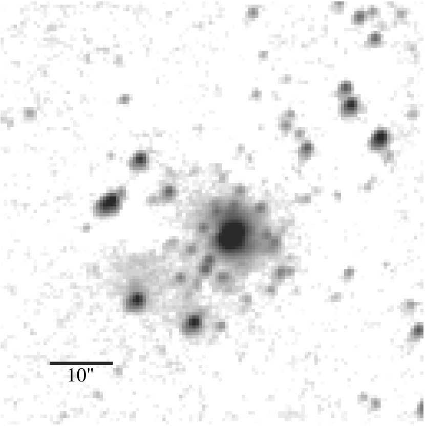
Figure 1: Log-scaled K^′ image of IRAS 06562$-$0337 obtained at Lick Observatory 3m telescope in March, 1997. Field of view is 70$\arcsec$ $\times$ 70$\arcsec$. North is up, East is to the left.

A log-scaled greyscale image of IRAS 06562$-$0337 with a field of view of 70$\arcsec$ $\times$ 70$\arcsec$ is presented in Figure 1. The image reveals a small, dense cluster of stars around a bright, central object. The association of the variable emission-line central object with a cluster of stars lends strong support to its classification as a young stellar object and not a PPN. Also evident is a diffuse nebulosity extending approximately 30$\arcsec$, whose brightness increases toward the central object. This nebulosity may be reflected light from the central object or the unresolved light from numerous low-mass stars in the cluster. The morphology of the faint nebulosity is somewhat affected by our choice of an on-source dithering pattern and the resulting sky subtraction. In particular, directly to the East of the central object, the apparent decrease in the brightness of the nebulosity is an artifact of the sky subtraction. The log-scaling emphasizes this low level data reduction artifact, which does not affect the results of this paper. An improved observing strategy for IRAS 06562$-$0337 would require chopping well away from the cluster to obtain sky images.

Our final image was photometered with the stand-alone DaophotII/AllstarII (Stetson, 1987). An empirical PSF was derived from 7 bright, fairly isolated stars with profile errors of order 3%. We obtained satisfactory star subtraction and PSF fitting photometry for all cluster stars except the central object. The seeing in our image measured with the PSF stars is 1.3$\arcsec$ (FWHM), while the central object has a FWHM of 1.5$\arcsec$. Thus we may be just resolving the central object. As conditions were not photometric, we can only crudely calibrate our photometry to K_CIT. Manchado et al. (1989) give K = 9.15 $\pm$ 0.02 mag for IRAS 06562$-$0337 obtained with a photometer and a beam width of 15$\arcsec$. This K magnitude is on the Tiede photometric system which is equivalent to K_CIT (Arribus and Martinez, 1987). We derived an aperture correction using a 15$\arcsec$ beam centered on the central object and the reported AllstarII magnitude. Given the slightly non-stellar profile of the central object, this procedure yields a rather large uncertainty of $\pm$ 0.2 mag for the zero-point transformation from our instrumental system to K_CIT. With the exception of the central object, our relative photometry of the cluster stars is more accurate. Typical AllstarII reported errors are K = 12.5 $\pm$ 0.03 mag, K = 16.5 $\pm$ 0.1 mag, and K = 18 $\pm$ 0.5 mag (see Fig. 2).

Artificial star tests were performed with DaophotII in 10 trials of adding 50 stars to our K^′ image, randomly distributed across the image and with magnitudes from K = 14 to 20. We find our completeness, defined as the ratio of stars recovered to stars added, is dependent on both magnitude and position. Considering artificial stars added at all positions in the image, we are approximately 95% complete at magnitudes brighter than K = 15, 90% complete at K = 16, and 50% complete at K = 17. At K = 18 we recovered almost no added stars. We find that within a radius of $\approx$ 5$\arcsec$ from the central object, we recovered no stars. Considering only artificial stars with K $<$ 17, we find our completeness to increase from approximately 85% around 10$\arcsec$ from the central object to nearly 100% at a radial position 60$\arcsec$ from the central object. This radial dependence of our completeness is attributable to both crowding and the irregular sky background contribution of the nebulosity.

2.2 Stellar Census

Our current near-infrared data is not ideal for a stellar census of IRAS 06562$-$0337. We primarily require a wider field of view (e.g. a mosaic image) to better characterize the foreground (and background) stars along this line of sight through the galactic plane. Nevertheless, as a first accounting of the cluster members we adopt a radius of 30$\arcsec$ as the cluster boundary, which is roughly the extent of the nebulosity seen in our K^′ image. Inside this radius we find 71 stars. Two equal area control fields, rectangular regions at the outer-most edges of our final image, contain 9 and 17 stars, predicting an average of only 13 background/foreground stars will be found inside our 30$\arcsec$ radius cluster boundary. We conclude that there is a significant stellar surface density enhancement in the immediate vicinity of IRAS 06562$-$0337. This confirms what may seem obvious from a casual inspection of Figure 1, that we have discovered a new star cluster.

In Figure 2, the top panel, we present the K luminosity function of stars found inside our 30$\arcsec$ radius cluster boundary. The cluster luminosity function is shown as the unshaded solid line histogram. The averaged luminosity function of our two control fields is shown as the shaded histogram. These two luminosity functions sample the same area of sky. Except for small differences in photometric completeness near the cluster center, they are properly comparable. A K-S test on the cluster and background luminosity functions gives a 1% probability that these are drawn from the same distribution. Corrections for completeness near the cluster center would result in even lower probabilities. Thus, in addition to the clustering in 2 dimensions on the sky, we find the K magnitude distribution of stars centered on IRAS 06562$-$0337 is not likely to be a statistical fluctuation in starcounts along this line-of-sight through the galactic plane.

In the bottom panel of Figure 2, we present the cluster luminosity function corrected for foreground/background stars and completeness. This luminosity function has 80 stars with K $<$ 17.5 mag. We have additionally overplotted theoretical luminosity functions corresponding to different initial mass functions (IMFs), parameterized by a power-law index $\alpha$. Our fiducial IMF is that of Salpeter (1955; $\alpha$ = 2.35), plotted as a solid line for K $<$ 17.5 mag and a long-dashed line for K $>$ 17.5 mag. A shallower and steeper IMF ($\alpha$ = 1.35 and 3.35, respectively) are also shown, as dotted lines. All three of the theoretical luminosity functions are normalized to have 80 stars for K $<$ 17.5 mag. We note that the steep IMF is the best fit, although without color information and comparisons to pre-main sequence isochrones, this analysis is susceptible to systematic biases. For instance, pre-main sequence stars will generally appear brighter at K than main sequence stars, biasing the IMF slope to higher values. We emphasize that our simple model luminosity functions demonstrate only a plausible, order-of-magnitude consistency between the observed cluster luminosity function and that expected from a Salpeter IMF. Nevertheless, this rough agreement supports the principal result of our paper, that IRAS 06562$-$0337 is a coeval young star cluster.

The theoretical luminosity functions allow us to estimate the K flux for an unresolved population of low-mass cluster stars, perhaps seen as the diffuse nebulosity in our image. The model luminosity functions, in this instance, can be regarded as empirical extensions of the observed luminosity function, and assigned no greater physical significance. Masking the central star (using IRAF) in an image with all other identified stars subtracted (using AllstarII), we find K_neb $\approx$ 11.3 mag inside a 30 $\arcsec$ beam. The measured flux of the nebulosity is quite sensitive to the adopted procedure of masking the central star. From several trials we estimate an uncertainty of roughly $\pm$ 0.5 mag. Excluding the central star (K = 9.2) the integrated magnitude of the stars in the histogram of the bottom panel of Figure 2 is K = 11.0 mag; including the central star we find K = 9.0 mag. Integrating the Salpeter IMF luminosity function beyond the last reliable bin in the completeness corrected luminosity function, from K = 17.5 to 23, gives K_neb,lf = 12.3 mag. Integrating the steep IMF from K = 17.5 to 23 gives K_neb,lf = 11.5 mag. We find the differences in K_neb,lf to be small when integrating to faint magnitude limits, changing only 0.2 mag when integrating to K = 21 or 23. Both of the predicted nebular fluxes are fainter than the measured flux, albeit with somewhat large uncertainties. Therefore, we might expect some contribution of reflected light from the central object to the nebulosity. Importantly, there is no gross inconsistency in our calculations, such as a prediction of too much diffuse light from faint stars. We conclude that our theoretical fit to the K luminosity function, extended to low mass stars (M $\approx$ 0.3 $M_{\odot}$), predicts an unresolved flux that is consistent with the brightness of the nebulosity observed in our K^′ image.

2.3 Mass and Size of IRAS 06562$-$0337

We adopt $K=-8\log(M/M_{\odot})+19.4$ for stars in the IRAS 06562$-$0337 cluster. The zero-point is estimated as follows. From Carpenter et al. (1997, see their Fig. 6), who compared near-IR data of the young star cluster Mon R2 to the pre-main sequence stellar evolution tracks of D’Antona and Mazzitelli (1994), we estimate an unreddened $M\approx 2.5M_{\odot}$ star would have K = 10.2 mag. Assuming a relative distance modulus between IRAS 06562$-$0337 and Mon R2 of 5 mag, and an IRAS 06562$-$0337 extinction of $A_{K}$ = 1 mag, yields the 19.4 mag zero-point. Our K mag/stellar mass calibration equates the bright central object, K = 9.2 mag, with an $M=18.8M_{\odot}$ star. Our mass estimate for the central star is consistent with an early B or late O spectral type (Mihalas and Binney, 1981). BGG estimate a B0-B2 spectral type from the luminosity, 21000 $L_{\odot}$. For comparison, GMSP calculate T_eff $\approx$ 3.6$\times$10⁴ K for the central star, which implies a late O spectral type (Mihalas and Binney, 1981).

Using the Salpeter IMF theoretical luminosity function to extend our observed luminosity function, we predict the following total numbers of cluster stars: 225, 445, 875, 1720, 3380 to the limiting magnitudes K = 19, 20, 21, 22, and 23 respectively. The total mass in the observed luminosity function is estimated by integrating the Salpeter IMF theoretical luminosity function to K = 17.5 which gives $M_{stars}$ $\approx$ 225 $M_{\odot}$. If we integrate to K = 23, we find $M_{stars}$ $\approx$ 1950 $M_{\odot}$, which compares with the lower limit of molecular gas mass given by BGG of $M_{gas}>1000M_{\odot}$. If a 50% mass-efficiency for star formation is adopted, we might expect the total mass of molecular gas in the cluster to be $M_{gas}$ $\approx$ 4000 $M_{\odot}$. Such a comparison is necessarily crude, particularly given our assumptions deriving the K mag/stellar mass calibration and extending a Salpeter IMF to the extreme lower main sequence and pre-main sequence.

IRAS 06562$-$0337 appears to be a large and rich young cluster. Similar young star clusters with massive Ae/Be central stars have been the subject of two recent surveys. Hillenbrand (1995) investigate the inner 0.3 pc of 17 clusters and find a linear relationship between central star mass and stellar surface density; Testi et al. (1997) study fields around 19 Herbig Ae/Be stars and report a correlation between spectral type and cluster richness, with earlier spectral types resulting in significantly more cluster stars, and some evidence of a threshold effect around spectral type B5–B7. Similar to Hillenbrand, they find a characteristic cluster radius to be 0.2 pc. At a distance of 7 kpc (BGG), our 30$\arcsec$ radius corresponds to a physical radius of 1 pc. This is $\sim$5 times the “typical” cluster radius, implying IRAS 06562$-$0337 is a very large cluster. The smallest distance estimate (2.4 kpc, GMSP) results in an adopted cluster radius of 0.34 pc, still $\sim 1.5-2$ times the “typical” value. Barsony et al. (1991) found 100 cluster members within $r\sim 1$ pc in the young star cluster LkH$\alpha$ 101, thus IRAS 06562$-$0337 is not unprecedented. We find an average stellar surface density of $\sim$25/pc² within 30$\arcsec$, increasing towards smaller radii. Testi et al. define a richness indicator, I_C, which measures the stellar density enhancement of a cluster, independent of cluster size, using K band starcounts. They find early type stars have I${}_{C}>10$, and MWC 137 (a B0 star) has the highest value in their sample, of I${}_{C}=76$. We estimate a value of I_C = 103 for IRAS 06562$-$0337. The high apparent mass of the central star is therefore consistent with the large size and richness of the IRAS 06562$-$0337 cluster.

2.4 Comparison of the K^′ Image and CO Map

We determined the coordinates of the central star by comparing the positions of 12 stars in our image with the Digitized Sky Survey image. The centroid of the central star at K^′ is offset slightly to the West of the visible image by $\Delta\alpha\sim$0.6$\arcsec$. Taking this into account, we found the two images to be in excellent agreement, with RMS scatter of less than 0.5$\arcsec$. Therefore, we report the J2000 K^′ (2$\micron$) position of the central object to be $\alpha$ = 06:58:44.31, $\delta$ = $-$03:41:09.97 (with uncertainties of $\pm 0.5\arcsec$). This differs by $\Delta\alpha=-$5.7$\arcsec$, $\Delta\delta=-$1.2$\arcsec$ from the near infrared position given by Manchado et al. (1989).

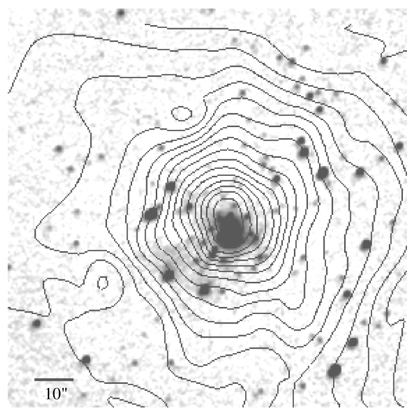
Figure 3: Log-scaled K^′ image of IRAS 06562$-$0337 obtained at Lick Observatory 3m telescope in March, 1997. Field of view is approximately 108$\arcsec$ $\times$ 108$\arcsec$. Contours are CO(2$\rightarrow$1) integrated line intensity from BGG, with the first contour level and subsequent step size equal to 10 K km s^-1.

Figure 3 presents the CO(2$\rightarrow$1) map of IRAS 06562$-$0337, graciously provided by BGG, overlaid on our K^′ image. The CO data was obtained in 1993 August and 1997 May with the IRAM 30-m telescope with a beam size of 12$\arcsec$ and an efficiency of 0.45 at 230 GHz. There is excellent agreement between the central peak of the CO emission and the central object in the K^′ image, even better than the agreement between the IRAS position and the CO emission pointed out by BGG. The peak in the CO emission and the central star are offset from each other by $\Delta\alpha=$0.6$\arcsec$, $\Delta\delta=$3.4$\arcsec$. The central contour of the CO plot is slightly elongated, extending 8.4$\arcsec$ E–W and 11.5$\arcsec$ N–S, which may imply a non-spherical molecular gas distribution. The majority of the emission (the first 12 contours) falls within 30$\arcsec$ of the central star, lending support to our choice of 30$\arcsec$ for the cluster radius, although strong emission ($>$ 5 K) extends over a region of $\sim 1\arcmin$ radius. The singly-peaked emission suggests that the central object in the K^′ image is the only massive young star in the cluster. The coincidence of the cluster stars and nebulosity seen in our K^′ image with the strong CO emission is strong evidence that the cluster is embedded in its placental molecular cloud (see also discussion in BGG).

The morphology of the molecular cloud around IRAS 06562$-$0337 sets it apart from other young clusters. Figure 3 clearly shows the CO distribution to be roughly spherically symmetric and well centered on the massive central star. Studies of Herbig Ae/Be clusters still associated with remnant molecular gas (Hillenbrand 1995, Barsony et al. 1991) do not generally find this to be the case. In fact, although the sample size is small, in almost every case the star appears to be located near the edge of the cloud, which is often elongated or otherwise shows signs of disruption. This may suggest interaction between the star and the cloud, such that the energy from the star is dispersing or disrupting the cloud (Hillenbrand 1995). We speculate that this implies extreme youth in the case of IRAS 06562$-$0337, where the parent molecular cloud is still in control, keeping the hot, young star snugly cocooned inside its dense layers.

3 Optical Spectroscopy

3.1 Observations and Data Reduction

On 1997 April 16 UT, we acquired 3 spectra of IRAS 06562$-$0337 from the Kast spectrograph (Miller & Stone 1993) on the 3m telescope at Lick Observatory. Spectrum #1 was exposed on the blue side of Kast for 900 seconds using the 600 line mm^-1 grism. Spectrum #2 was exposed concurrently on the red side of Kast for 900 seconds using the 830 line mm^-1 grating. Spectrum #3 was exposed on the red side of Kast for 600 seconds, approximately 35 minutes after the other spectra, using the 600 line mm^-1 grating. All three spectra were taken through a 2 arcsec slit. The spectra were reduced and extracted using standard IRAF routines (Massey, Valdes, & Barnes 1992). They were wavelength-calibrated using a HeHgCd arc lamp spectrum for the blue spectrum (#1), and a HeNeAr arc lamp spectrum for the red spectra (#’s 2 and 3). Fine corrections to the zero points of the wavelength scales were made via inspection of the night sky lines. The resultant wavelength coverage and resolution (mean FWHM of lines in the corresponding arc spectrum) for each spectrum are 3095–5206Å (resolution 3.2Å) for spectrum #1, 6028–8061Å (resolution 4.2Å) for spectrum #2, and 4274–7059Å (resolution 5.5Å) for spectrum #3. The instrumental response function was removed from the spectra and they were flux-calibrated using observations of spectrophotometric standard stars obtained on the same night with the same grating settings; Feige 34 (Massey et al. 1988) was used for spectrum #1 and HD 84937 (Oke & Gunn 1983) for spectra #’s 2 and 3.

A composite spectrum of IRAS 06562$-$0337 is shown in Figure 4. It combines the data from 3100–5200Å in spectrum #1, 5200–7050Å in spectrum #3, and 7050–8050Å in spectrum #2. The bottom panel of Figure 4 shows the full wavelength and flux scales of the composite spectrum. The most prominent feature is a very strong emission line of H$\alpha$ that dwarfs any other spectral features. The continuum level increases to the red. A power law fit to the continuum, $F_{\lambda}\propto\lambda^{\alpha}$, gives an index of $\alpha\approx 2.5$. In the middle panel of Figure 4, we have reduced the range of the flux axis so that the weaker features are more apparent. The first three Balmer lines and several terrestrial atmospheric features are indicated. We were able to identify Balmer lines all the way to H11 ($\lambda 3771$); blueward of H$\delta$, the Balmer lines are in absorption rather than emission. Although the spectrum becomes somewhat noisy at its blue end, a small central emission component (peaking well below the local continuum level) is apparent in the bottom of each of the H$\epsilon$–H11 absorption lines. This suggests that the Balmer profiles in IRAS 06562$-$0337 are made up of at least two components: an absorption line and a superposed emission line. The absorption depth does not change greatly from H$\epsilon$ to H11, but the intensity of the emission component increases up the Balmer series such that the lines switch from mostly absorption at H$\epsilon$ to mostly emission at H$\delta$. This is qualitatively similar to the Balmer emission observed in other Be stars (Burbidge and Burbidge, 1953). In the top panel of Figure 4 the wavelength and flux scales of the composite spectrum are expanded, with several typical features labeled. In addition to the Balmer lines and diffuse interstellar bands (DIBs; Herbig 1975), we find several absorption lines of He I and many (permitted and forbidden) emission lines of metals. Most of the latter are lines of Fe II and [Fe II]; the remainder are Si II and [O I]. There are a few unidentified and/or extremely weak features in the composite spectrum; hence, we cannot rule out the possible presence of lines of other elements or additional lines of the identified elements.

Tables 1a, 1b, and 1c list the equivalent widths (EWs) and integrated fluxes for the identifiable lines and DIBs in each of the spectra. The EWs and fluxes were measured via direct integration of pixel values between manually-selected endpoints in the flux-calibrated spectra. Several trials of each measurement were accomplished to estimate the uncertainty; in general, the measurements are accurate to $\pm 10\%$ or better (values with larger probable uncertainties are denoted with a “:”). A negative flux value in the tables indicates an absorption line.

3.2 Spectral Analysis and 1996–1997 Variablity

The 1996 (KLR) and 1997 (this paper) epoch spectra have similar resolution and high S/N, which allows the first investigation of the variability of many fainter lines. In Table 2 we have assembled select emission line strengths from our Tables 1a,b,c and KLR (1996, their Table 1) to make the comparison. Lines are included in Table 2 if they are relatively unblended in our 1997 epoch spectra (typical uncertainties of 10% in the line fluxes) and were also identified in the KLR spectrum. In some instances, particularly useful lines, such as the [O I] lines, were included despite their larger flux uncertainties. In these cases, we mantain the use of the “:” as in Tables 1a,b,c to designate the larger uncertainty. In other cases, the flux of two blended lines of the same ionization species are listed for 1997, and the combined flux of the two resolved lines in the KLR spectrum is listed for 1996. KLR do not report absolute fluxes, so we have normalized the fluxes to H$\beta$ = 100. In the bottom part of Table 2, we have listed several line ratios; typical uncertainties are 14% unless otherwise discussed below.

KLR suggest that the variable emission seen by GMSP may be understood as a patchy circumstellar envelope around a single star. Using the Balmer decrements, we investigate the hypothesis that variable extinction, possibly due to orbiting dust clouds, could mimic variable emission between 1996 and 1997. We estimate the uncertainties in our flux measurements for the H$\alpha$, H$\beta$ and H$\gamma$ Balmer lines is $\approx$ 5%, or 7% in the ratios. KLR do not report uncertainties; however, we will assume they are 10%, or 14% in the ratios. To derive the extinction, we adopt the intrinsic decrements H$\alpha$/H$\beta$ = 2.80 and H$\gamma$/H$\beta$ = 0.47 from Osterbrock’s (1974) compilation of Case B recombination line ratios, appropriate for a temperature near 2$\times$10⁴ K (GMSP), and the reddening law of Cardelli, Clayton, and Mathis (1987). For 1997 we find $A_{V}$ = 8.15 $\pm$ 0.25 and $A_{V}$ = 8.6 $\pm$ 0.4 from H$\alpha$/H$\beta$ and H$\gamma$/H$\beta$ respectively. Similarly, for 1996 we find $A_{V}$ = 8.35 $\pm$ 0.4 and $A_{V}$ = 8.2 $\pm$ 0.9. The weighted average of all four measurements gives $A_{V}$ = 8.3 $\pm$ 0.35 mag, or a color excess of $E(B-V)$ = 2.68 $\pm$ 0.12 mag. Note that our estimate of the uncertainty does not include a contribution from the reddening law or the adopted intrinsic line ratios. The color excesses derived in 1996 and 1997 agree well, which implies a negligible change in extinction over the one year interval. Our color excess can be compared with that derived by GMSP of $E(B-V)$ = 1.75 $\pm$ 0.25 mag. The discrepancy is significant, and may be due to different assumptions in the reddening law or intrinsic line ratios or a real change in the extinction between 1990 and 1996/1997. GMSP do not give observed line fluxes, only dereddened fluxes, and do not describe their procedure for calculating the reddening in detail. For these reasons, we do not make any additional comparisons to the GMSP spectral line data. Lastly, the Cardelli, Clayton, and Mathis reddening law gives $A_{K}$ = 0.114$\times$$A_{V}$, or $A_{K}$ = 0.95 mag for IRAS 06562$-$0337, which is what we assumed in Section 2.

Keenan et al. (1995) present an [O I] (6300+6364/5577) temperature and density diagnostic diagram, as do Bautista and Pradhan (1995). In our data, the $\lambda 6364$ and $\lambda 5577$ lines were both blended and have large uncertainties, estimated to be approximately 30%. The [O I] (6300+6364/5577) line ratio (see Table 2) is consistent with no change over the 1996 to 1997 interval, although this result is fairly uncertain. It is noteworthy that the unblended and strong [O I] $\lambda 6300$ line intensity decreased by a factor of two over this year (a high significance), yet the [O I] line ratio remained constant. We derive log($n_{e}$) $\approx$ 5.8 assuming an electron temperature, $T_{e}$ = 2$\times$10⁴ K (GMSP). We additionally derive an upper limit to the electron density, log($n_{e}$) $\leq$ 15.45, from the Inglis-Teller formula (1939) and our observation of the H11 Balmer line. Our use of the Inglis-Teller formula is limited by the noise at the blue end of our spectra. For comparison, Viotto (1976) tabulated electron densities and temperatures for a number of Be stars. They are typically $n_{e}\approx 4\times 10^{11}$ cm^-3 and $T_{e}\approx$ 1-2$\times 10^{4}$ K, with earlier spectral types having the higher electron temperatures. The (low) electron density derived from the [O I] line ratio implies an origin for these lines at the “outskirts” of the ionized region. This may reflect a partially ionized zone at the edge of a wind-swept ionized cavity (e.g. Barsony et al. 1990, Becker and White, 1988) or the “outer wind” analagous to that seen in P Cygni (Stahl et al. 1991).

GMSP argued that their time-series of spectral data imply an increasing temperature, consistent with a rapidly evolving central star in a PPN. We consider whether the 1996–1997 spectral line variability can be understood as simple changes in electron temperature or density. The permitted lines of Fe II and Si II show a general trend of decreasing intensity over the 1996 to 1997 interval. Of five lines selected for comparison, one line (Fe II $\lambda 5018$) shows an $\approx$ 1$\sigma$ increase, while four other lines show 1-2$\sigma$ decreases. The average decrease in line intensity is 80%. If the permitted lines of Fe II and Si II behave similarly to the hydrogen and helium recombination lines, then their intensities depend very weakly on electron density (e.g. collisional effects, Osterbrock 1974), and with a temperature dependence,

$$I(recombination)\propto T_{e}^{-1.1}$$ (1)

(Oliva et al., 1989). This implies an increase in the electron temperature of approximately 20% in one year. Assuming an initial electron temperature of $2\times 10^{4}$ K, the increase would be $\Delta$$T_{e}\approx+4500$ K. The most dramatically varying line in Table 2 is [O I] $\lambda 6300$, which decreased by a factor of two (approximately 5$\sigma$) between 1996 and 1997. The electron temperature and density dependence of this forbidden line is given by:

$$I(forbidden)\propto n_{e}n_{ion}\Omega(T)T_{e}^{-1/2}10^{-T_{\lambda}/T_{e}}$$ (2)

where $T_{\lambda}$ = c2/$\lambda$, c2 is the second radiation constant (1.438769 cm K) and $\lambda$ is in units of cm; for [O I] $\lambda 6300$, T_λ = 22837. $\Omega$(T) is the collision strength which we will assume has a weak temperature dependence (Osterbrock 1974), $n_{e}$ is the electron density, and $n_{ion}$ is the density of the ion species, in this case, neutral oxygen. A change in the electron density of 0.2 dex is reasonably allowed by the uncertainty of our [O I] line ratio. Therefore, we cannot rule out a factor of two decrease in the electron density as the cause of the factor of two decrease in the [O I] $\lambda 6300$ line intensity. If the flux variability is entirely due to a change in temperature, we find $\delta$$T_{e}\approx+9000$ K, with an estimated uncertainty of about 5000 K, consistent with the temperature change implied by the permitted lines. However, an apparent temperature increase of $\sim$5000 K in one year seems unlikely to be related to stellar evolution (the suggestion of GMSP, KLR), and rather implies more complex physical processes.

The intensity of all lines of [Fe II] listed in Table 2 increased between 1996 and 1997 and appear anti-correlated with the intensities of the [O I] lines, which decreased in the same interval. Typically, a positive correlation is found between [O I] and [Fe II] emission strength in a wide range of objects including supernova remnants, Seyfert galaxies, and H II regions such as Orion (Bautista and Pradhan, 1997, 1995; Bautista, Pradhan and Osterbrock 1994; Mouri et al. 1990). In these objects, [O I] emission is believed to originate in partially ionized zones (PIZs), lying at the edges of fully ionized zones. The [O I]/[Fe II] correlation is attributed to the filling factor of the PIZs and the coincidence of the [O I] and [Fe II] species in the PIZs. In IRAS 06562$-$0337, a simple change in the electron temperature or density will not explain the behavior of both the [O I] and [Fe II] lines. It is conceivable that dust grains are being blown away and iron depleted onto the grains is being returned to a gas state, enough to offset the effect of an increasing temperature. An alternative, and preferred, explanation is that the [O I] and [Fe II] emission are not originating in the same zone, which argues against a presumably static shell-like PIZ at the edge of a wind-swept cavity and favors a more dynamic “outer wind” origin for these forbidden lines. Lastly, we note that the suggestion of KLR that the [Fe II] emission is due to flourescence is unlikely at densities of log($n_{e}$) $\approx$ 5.8, as shown by Bautista, Peng, and Pradhan (1996).

4 Conclusions

The bright central object in IRAS 06562$-$0337 is probably a single Herbig Ae/Be class star, with $M\approx 20M_{\odot}$. There is some evidence that it is seen at least partially in reflection. For example, the central star is poorly fit by the stellar point spread function derived from other stars in our K^′ image. In addition, the centroids in the visible and at K^′ are offset by $\Delta\alpha\sim$0.6$\arcsec$. A comparison of our 1997 epoch optical spectra to the 1996 epoch spectrum presented by KLR has provided new evidence for spectral line variability in IRAS 06562$-$0337 that is not easily interpreted as simple changes in temperature or density. This argues against previous suggestions that the already-published spectral data reflect real-time evolutionary changes of the central star. Understanding the immediate environs of the central star is an essential first step to better understanding the emission line variability that has been observed.

We note that our analysis of the 1996–1997 spectral variability of IRAS 06562$-$0337 using simple zones and changes in one parameter (such as the electron temperature or electron density) is only intended as an interpretive tool and should be treated with some caution. The inconsistencies of this analysis suggest the complexity of the actual emission line region. If the central star is analagous to a Herbig Be star, then its “fully ionized zone” should have a very high electron density. Thus, the low density derived with the [O I] emission implies a stratification of densities, likely in the extended atmosphere of the central star in IRAS 06562$-$0337. The anti-correlation of [O I] and [Fe II] emission is not easily understood if they arise from a common partially ionized zone (perhaps located at the edge of a compact H II region around the central star), but is likely consistent with an origin in a dynamic stratified atmosphere. Spectral variability is also consistent with a stellar wind origin. Stellar winds from Herbig Be type stars are highly variable, extremely complex, and poorly understood (e.g., they are possibly modulated by magnetic fields or non-radial pulsations; Catala et al. 1993). Wind line strengths and profiles can show nightly variations, some of which are correlated with temperature changes of the star (Scuderi et al. 1994). The appearance of [O III] emission in IRAS 06562$-$0337 during 1990 (GMSP) can be understood as shocks in stellar jets from a variable stellar wind (Hartigan & Raymond 1993). Additionally, we emphasize that the size of the ionized region in IRAS 06562$-$0337 is small. Six cm radio observations yielded a surprising non-detection given the strong H$\beta$ flux, and allow an upper limit angular diameter of $3.4\times 10^{-4}$ arcsec to be set for the ionized region (GMSP). If we assume the 7 kpc distance estimate of BGG, then the ionized region in IRAS 06562$-$0337 has an upper limit diameter of 2–3 AU. We conclude that stellar winds in the extended, stratified atmosphere of a very young, $M\approx 20M_{\odot}$ star is the most plausible explanation for the puzzling spectral variability of IRAS 06562$-$0337, the “Iron Clad Nebula.”

A valuable time series of spectra of the central object in IRAS 06562$-$0337, covering a 10 year interval, are now available in the literature. A useful complementary study would obtain more densely sampled spectroscopic observations, to investigate the short timescale behavior of the emission. In particular, correlated line variability and characteristic timescales could be used to constrain the dimensions of the ionized region, which we have suggested is likely to be an extended stellar atmosphere. We emphasize the need for high resolution and high S/N spectroscopic observations in the near-UV, and of the entire Balmer series, as these data can be used to study the extended atmospheres of Be stars (Burbidge & Burbidge 1953). It is important to build a consistent physical picture of the environs around the central star in order to answer questions such as “is the central star seen in reflection?” This problem in particular could be addressed with high resolution imaging and polarization data. Lastly, as a young star cluster, IRAS 06562$-$0337 is interesting and notable for its richness. Multi-color near-infrared photometric observations would allow an accurate measurement of the IMF, and an investigation into problems such as mass segregation and star formation efficiencies (e.g., Barsony et al. 1991).

5 Acknowledgments

Alves’ research at a DOE facility is supported by an Associated Western Universities Laboratory Graduate Fellowship. Work at LLNL performed under the auspices of the USDOE contract no. W-7405-ENG-48. Hoard’s research supported by NSF grant no. AST 9217911. Alves and Hoard thank our respective advisors, Kem Cook and Paula Szkody. Rodgers is supported by the NASA Graduate Student Research Program, and thanks her advisors Bruce Balick and Diane Wooden. Alves acknowledges Thor Vandehei for his exuberant assistance while observing at the Lick Observatory. We also thank Bob Becker, Hien Tran, Carlos de Breuck, and Bill Latter for their useful comments and discussions that significantly improved this paper.

Table 1: Spectrum #1

$\lambda_{obs}$	EW	Flux
(Å)	(Å)	($\times 10^{-15}$ erg s-1 cm-2)	Identification
3774	1.8	$-$1.6+	H I $\lambda 3771$ (H11)
3797	1.3	$-$1.2+	H I $\lambda 3798$ (H10)
3812	1.1	1.0	Fe II $\lambda 3814$
3837	2.0	$-$2.0+	H I $\lambda 3835$ (H9)
3856	1.4	1.4	Si II $\lambda\lambda 3854,3856$
3892	2.1	$-$2.1+	He I $\lambda 3889$, H I $\lambda 3889$ (H8)
3916	string0.9:	string0.9:	Fe II $\lambda 3915$
3973	3.0	$-$3.0+	H I $\lambda 3970$ (H$\epsilon$)
4100	1.0	1.1	H I $\lambda 4102$ (H$\delta$)
4170	string0.8:	string1.0:	Fe II $\lambda 4170$
4245	string0.9:	string1.1:	[Fe II] $\lambda 4244$
4340	2.8	3.7	H I $\lambda 4341$ (H$\gamma$)
4390	string0.7:	string$-$1.0:+	He I $\lambda 4388$
4415	0.9	1.2	[Fe II] $\lambda 4414$,Fe II $\lambda 4417$
4430	2.1	$-$2.9+	DIB 4428Å
4472	string0.4:	string$-$0.6:+	He I $\lambda 4471$
4494	string0.4:	string0.6:	Fe II $\lambda 4491$
4503	string0.2:	string$-$0.3:+	DIB 4502Å
4584	0.5	0.7	Fe II $\lambda\lambda 4584$
4716	string0.2:	string$-$0.4:+	He I $\lambda 4713$
4731	string0.3:	string0.4:	Fe II $\lambda 4731$
4817	0.6	1.0	Fe II $\lambda 4818$,[Fe II]
4863	18.10	31.70	H I $\lambda 4861$ (H$\beta$)
4883	0.6	$-$1.1+	DIB 4882Å
4891	string0.4:	string0.7:	Fe II $\lambda 4894$
4924	0.6	1.0	Fe II $\lambda 4924$
5020	1.0	2.0	Fe II $\lambda 5019$
5044	0.3	0.7	Si II $\lambda 5041$
5058	string0.5:	string1.1:	Si II $\lambda 5056$
5151	string0.3:	string0.6:	Fe II $\lambda 5149$
5160	string1.6:	string3.6:	[Fe II] $\lambda\lambda 5158,5159$
5169	string1.6:	string3.6:	Fe II $\lambda 5169$

Table 2: Spectrum #3

$\lambda_{obs}$	EW	Flux
(Å)	(Å)	($\times 10^{-15}$ erg s-1 cm-2)	Identification
4436	string3.4:	string$-$4.7:+	DIB 4428Å
4475	string1.4:	string$-$1.9:+	He I $\lambda 4471$
4820	string1.3:	string 2.1:	Fe II $\lambda 4818$, [Fe II]
4868	19.00	32.00	H I $\lambda 4861$ (H$\beta$)
5026	1.0	1.9	Fe II $\lambda 5018$
5164	string1.6:	string3.5:	[Fe II] $\lambda\lambda 5158,5159$
5174	string1.6:	string3.5:	Fe II $\lambda 5169$
5204	string0.4:	string0.9:	Fe II $\lambda 5198$
5267	string1.7:	string4.0:	[Fe II] $\lambda 5269$
5277	string1.7:	string4.0:	[Fe II] $\lambda 5278$
5337	0.8	2.0	[Fe II]
5380	0.5	1.3	[Fe II]
5579	string0.2:	string0.6:	[O I] $\lambda 5577$
5706	0.5	$-$2.0+	DIB 5705Å
5750	string0.6:	string1.7:	[Fe II] $\lambda 5747$
5754	string0.6:	string1.7:	[Fe II] $\lambda 5754$
5780	1.3	$-$4.0+	DIB 5778,5780Å
5797	string0.3:	string$-$0.8:+	DIB 5797Å
5870	0.8	2.5	Fe II$\lambda 5865$
5891	string2.6:	string$-$8.4:+	Na I $\lambda 5890$ (D-lines)
5897	string 2.6:	string$-$8.4:+	Na I $\lambda 5896$ (D-lines)
5951	string0.6:	string2.1:	Si II $\lambda 5949$
5959	string0.6:	string2.1:	Si II $\lambda 5958$
5980	0.6	1.9	Si II$\lambda 5980$
6048	string0.4:	string1.4:	[Fe II]
6126	string0.4:	string1.5:	Fe II $\lambda 6130$
6284	3.2	$-$11.7+0	DIB 6284Å
6302	1.1	4.1	[O I] $\lambda 6300$
6320	0.6	2.4	Fe II
6348	0.6	2.2	Si II $\lambda 6347$
6365	string0.9:	string3.5:	[O I] $\lambda 6364$
6374	string0.9:	string3.5:	Si II $\lambda 6371$
6386	0.7	2.8	Fe II $\lambda 6384$
6443	string0.7:	string2.9:	Fe II $\lambda 6446$
6564	302000	12650000	H I $\lambda 6563$ (H$\alpha$)
6615	string0.4:	string$-$1.8:+	DIB 6614Å
6659	string1.1:	string$-$4.9:+	DIB 6661Å
6681	string0.4:	string$-$1.8:+	He I $\lambda 6678$

Table 3: Spectrum #2

$\lambda_{obs}$	EW	Flux
(Å)	(Å)	($\times 10^{-15}$ erg s-1 cm-2)	Identification
6250	string0.2:	string0.5:	Fe II $\lambda 6248$
6286	3.0	$-$11.8+0	DIB 6784Å
6303	1.3	4.9	[O I] $\lambda 6300$
6320	string0.6:	string2.2:	Fe II
6348	0.7	2.8	Si II $\lambda 6347$
6366	string0.8:	string3.1:	[O I] $\lambda 6364$
6371	string0.8:	string3.1:	Si II $\lambda 6371$
6388	0.8	3.3	Fe II $\lambda 6384$
6443	string0.2:	string0.9:	Fe II $\lambda 6446$
6565	283000	11430000	H I $\lambda 6563$ (H$\alpha$)

Table 4: Comparison of 1996 and 1997 Epoch Spectra

Line Flux or Flux Ratio	1997	1996
H I $\lambda 4341$ (H$\gamma$)	11.5	12.2
H I $\lambda 4861$ (H$\beta$)	100	100
Fe II $\lambda 5018$	5.9	5.1
[Fe II] $\lambda 5269+\lambda 5278$	12.5	11.9
[Fe II] $\lambda 5334$	6.3	3.2
[Fe II] $\lambda 5380$	4.1	3.1
[O I] $\lambda 5577$	string1.9:	4.5
[Fe II] $\lambda 5747+\lambda 5754$	5.3	2.2
Si II$\lambda 5980$	5.9	7.1
[O I] $\lambda 6300$	12.8	23.5
Fe II $\lambda 6320$	7.5	12.7
Si II $\lambda 6347$	6.8	8.6
Fe II $\lambda 6384$	8.8	12.3
H I $\lambda 6563$ (H$\alpha$)	3953	4221
[O I] $\lambda 6364$	string5.5:	6.3
H$\alpha$/H$\beta$	39.5	42.2
H$\gamma$/H$\beta$	0.115	0.122
[O I] (6300+6364/5577)	8.0	6.6
[O I] $\lambda 6300$/[Fe II] $\lambda 5334$	2.0	7.3

Figure 2: Top panel shows K luminosity function of stars inside radius of 30$\arcsec$ around central object of IRAS 06562$-$0337 (71 stars, unshaded histogram) and average of two equal area control regions (13 stars, shaded histogram). Completeness is 90% at K = 16 mag. Bottom panel shows the cluster luminosity function corrected for background/foreground stars and completeness (histogram) and three model luminosity functions (lines, see text).

Figure 4: The composite optical spectrum of IRAS 06562$-$0337. The bottom panel shows the full wavelength and flux scales of the spectrum. The middle panel shows the spectrum with an expanded flux scale. Several Balmer emission lines and terrestrial atmospheric absorption features are marked. The top panel shows a segment of the spectrum with expanded scales of both wavelength and flux. A number of typical features are marked.