The Distribution of Nearby Stars in Velocity Space
Inferred from Hipparcos Data

Abstract

The velocity distribution $f(\mbox{\boldmath$v$})$ of nearby stars is estimated, via a maximum-likelihood algorithm, from the positions and tangential velocities of a kinematically unbiased sample of 14 369 stars observed by the HIPPARCOS satellite. $f$ shows rich structure in the radial and azimuthal motions, $v_{R}$ and $v_{\varphi}$, but not in the vertical velocity, $v_{z}$: there are four prominent and many smaller maxima, many of which correspond to well known moving groups. While samples of early-type stars are dominated by these maxima, also up to about a quarter of red main-sequence stars are associated with them. These moving groups are responsible for the vertex deviation measured even for samples of late-type stars; they appear more frequently for ever redder samples; and as a whole they follow an asymmetric-drift relation, in the sense that those only present in red samples predominantly have large $|v_{R}|$ and lag in $v_{\varphi}$ w.r.t. the local standard of rest (LSR). The question arise, how these old moving groups got on their eccentric orbits? A plausible mechanism known from the solar system dynamics which is able to manage a shift in orbit space is sketched. This mechanism involves locking into an orbital resonance; in this respect is intriguing that Oort’s constants, as derived from HIPPARCOS data, imply a frequency ratio between azimuthal and radial motion of exactly $\Omega:\kappa=3:4$.

Apart from these moving groups, there is a smooth background distribution, akin to Schwarzschild’s ellipsoidal model, with axis ratios $\sigma_{R}:\sigma_{\varphi}:\sigma_{z}\approx 1:0.6:0.35$. The contours are aligned with the $v_{r}$ direction, but not w.r.t. the $v_{\varphi}$ and $v_{z}$ axes: the mean $v_{z}$ increases for stars rotating faster than the LSR. This effect can be explained by the stellar warp of the Galactic disk. If this explanation is correct, the warp’s inner edge must not be within the solar circle, while its pattern rotates with frequency $\gtrsim 13\mbox{$\,{\rm km}\,{\rm s}^{-1}\,{\rm kpc}^{-1}$}$ retrograde w.r.t. the stellar orbits.

accepted for publication by the Astronomical Journal

1 INTRODUCTION

The dynamical state of a stellar system is completely described by its phase-space distribution function $F(\mbox{\boldmath$x$},\mbox{\boldmath$v$})$. Knowledge of that function allows one to derive the underlying gravitational potential and hence the mass distribution, since in equilibrium $F$ must be constant on the orbits supported by the potential. Furthermore, one can try to understand $F$ in terms of the possible formation history and evolution of the stellar system under study. Unfortunately, $F$, being a six-dimensional function, is impossible to measure for any remote galaxy; all one can hope is to measure a three-dimensional projection, and even this requires spectra to be taken at all positions on the galaxy. For the Milky Way the situation is completely different. In a sense it is worse, since we cannot observe a clean and easily predictable projection. Rather we observe individual stars and are in danger of seeing the trees for the wood. However, if we forget individual stars and observe large samples, we can actually measure $F(\mbox{\boldmath$x$},\mbox{\boldmath$v$})$ itself, at least in principle. The problem here is the shear amount of labour necessary to collect accurate measurements of stellar phase-space coordinates for large samples, in particular of faint stars. This has so far prevented this route from being used. Thus, we must either restrict ourselves to luminous and hence young stars, or to very nearby stars of all stellar types and ages. Since young stars are more likely to have not yet settled into equilibrium, interpretation of their phase-space distribution is more complicated. The best we can currently hope to get for the old stellar population is the velocity distribution in the solar neighborhood $f(\mbox{\boldmath$v$})\equiv F(\mbox{\boldmath$x$}{=}\mbox{\boldmath$x$}_{\odot},\mbox{\boldmath$v$})$.

Historically, there are two divergent approaches to $f(\mbox{\boldmath$v$})$. One is mainly based on theoretical lines of argument like the epicycle approximation and dynamical heating mechanisms. It manifests itself in Schwarzschild’s (1908) ellipsoidal distribution, i.e. $f(\mbox{\boldmath$v$})$ is assumed to be smooth, single-peaked, and well described by the mean velocity and dispersion in conjunction with Strömberg’s asymmetric drift relation (cf. Binney & Tremaine 1987, p. 198 and 202). The other approach to $f(\mbox{\boldmath$v$})$ is more observational and mainly restricted to luminous stars on account of magnitude limits. It begins with Kapteyn’s (1905) recognition of moving groups, which were later studied in more detail by Eggen (1965 and references therein, 1995, 1996). That is, $f(\mbox{\boldmath$v$})$ for early-type stars appears to be dominated by several independent components. According to the standard interpretation, stars of a moving group have formed simultaneously in a small phase-space volume. The idea is that phase mixing and scattering processes have not yet completely washed out the initial correlation of the moving group, and we can still observe a stream of stars with similar velocities. The old stellar populations, on the other hand, should be completely mixed and obey a smooth distribution function. This interpretation, however, is merely hypothetical and by no means proven. Indeed, the results of this paper raise problems for this simple picture.

ESA’s astrometric satellite HIPPARCOS ([ESA 1997]) provided us with positions and trigonometric parallaxes of unprecedented accuracy for tens of thousands of stars near the Sun. From these data we can, for the first time in history, extract large and homogeneous stellar samples with accurately known distances and, what is important, completely free of the kinematic biases that have plagued similar studies in the past. Since HIPPARCOS has additionally measured the absolute proper motions for the same stars, it offers us the opportunity to investigate in some detail the nature of the velocity distribution in the solar neighborhood not only for early-type stars but also for the old stellar population of the Galactic disk. In a preceding paper (Dehnen & Binney 1998b, hereafter paper I), we have used a kinematically unbiased subsample of the HIPPARCOS Catalogue to infer, as a function of stellar color, the first two moments, mean and dispersion, of $f(\mbox{\boldmath$v$})$ for nearby stars. This paper goes beyond these moments to infer the velocity distribution itself from the HIPPARCOS data.

If the HIPPARCOS mission were complemented by a program to measure the radial velocities of the same stars, we could obtain to high accuracy their space velocities $v$, and hence directly measure the distribution function for these stars. Unfortunately, however, the radial velocities for many stars in the HIPPARCOS Catalogue are not (yet) publicly known. From the existing literature one can extract radial velocities only for a subset of HIPPARCOS stars that is heavily kinematically biased in the sense that it predominantly contains high-proper-motion stars ([Binney et al. 1997]). Hence, in order to make full use of the HIPPARCOS Catalogue, or of similar future catalogs, for studies of stellar kinematics, one cannot necessarily rely on radial velocities, but must be able to work with the positions and tangential velocities alone. For each position on the sky, the tangential velocity is a certain combination of the components of the space velocity. It is immediately clear that we can only proceed if we link together the tangential velocities measured for stars in different directions from the Sun. In order for such a method to be valid, one must make the basic assumption that $f(\mbox{\boldmath$v$})$ is independent of the position on the sky, a condition that should be satisfied for sufficiently nearby stars.

In Section 2, I show that, under this basic assumption, knowing the distributions of tangential velocities for a region of the celestial sphere that cuts all great circles gives complete knowledge of the full distribution of space velocities. The problem is formally equivalent to that of classical tomography. However, there is a fundamental difference, namely that we are unable to measure the distributions of tangential velocities to arbitrary accuracy, rather we only know the tangential velocities for a few thousand stars distributed over the sky. Consequently, we cannot use the tools developed for tomography. Instead, in Section 3, a maximum-likelihood technique is presented and tested that enables one to estimate $f(\mbox{\boldmath$v$})$ for a set of stars from their positions, parallaxes, and proper motions.

The reader not interested in these techniques and numerical details but mainly in the resulting $f(\mbox{\boldmath$v$})$ may skip Sections 2 and 3 and directly go to Section 4, where the algorithm is applied to the kinematically unbiased subsample of HIPPARCOS stars that we have already used in paper I. The results and their implications are discussed in Sections 5 and 6, while Section 7 sums up.

2 THE PROJECTION OF SPACE VELOCITIES

2.1 The Projection Equations

Let $v$ be the velocity of a star w.r.t. the Sun in a Cartesian coordinate system with $v_{x}$, $v_{y}$, and $v_{z}$ denoting the motions towards the Galactic center, in the direction of Galactic rotation, and towards the north Galactic pole, respectively. While this coordinate system is a good choice in dynamical studies, the natural coordinates for observations are $v_{r}=\dot{r}$, $v_{\ell}=r\mu_{\ell}\cos b$, and $v_{b}=r\mu_{b}$. Here $\ell$, $b$, and $r$ denote, respectively, Galactic longitude, latitude, and distance from the Sun. $\mu_{\ell}$ and $\mu_{b}$ are the proper motions corrected for the effects of Galactic rotation

$$\begin{array}[]{r@{\,=\,}l}\mu_{\ell}&\mu_{\ell}^{\rm(obs)}-A\,\cos(2\ell)-B\\ \mu_{b}&\mu_{b}^{\rm(obs)}+A\,\sin(2\ell)\,\cos b\,\sin b,\end{array}$$ (1)

with Oort’s constants $A$ and $B$; I use Feast & Whitelock’s (1997) values (in $\,{\rm km}\,{\rm s}^{-1}\,{\rm kpc}^{-1}$) $A=14.82$ and $B=-12.37$ obtained from HIPPARCOS Cepheids, but the results are insensitive to the precise values. The two coordinate systems are related by a rotation

$$(v_{r},v_{\ell},v_{b})^{T}={\bf R}\cdot\mbox{\boldmath$v$},\qquad\mbox{\boldmath$v$}={\bf R}^{T}\!\cdot(v_{r},v_{\ell},v_{b})^{T}$$ (2)

with rotation matrix

$${\bf R}=\left[\begin{array}[]{r@{\quad}r@{\quad}r}\cos b\,\cos\ell&\cos b\,\sin\ell&\sin b\\ -\sin\ell&\cos\ell&0\\ -\sin b\,\cos\ell&-\sin b\,\sin\ell&\cos b\end{array}\right].$$ (3)

For our purposes it is useful to consider the two-dimensional velocity vector $\mbox{\boldmath$q$}\equiv(v_{\ell},v_{b})$, which can be evaluated from HIPPARCOS’s measurements. It is related to $v$ by the projection equation

$$\mbox{\boldmath$q$}={\bf S}\cdot\mbox{\boldmath$v$}$$ (4)

where the $2\times 3$ matrix ${\bf S}$ is given by the second and third row of ${\bf R}$. In the $(v_{x},v_{y},v_{z})$ frame, the corresponding tangential velocity $\mbox{\boldmath$p$}\equiv{\bf S}^{T}\cdot\mbox{\boldmath$q$}$ is related to $v$ by the projection

$$\mbox{\boldmath$p$}=\mbox{\boldmath$v$}-(\hat{\mbox{\boldmath$r$}}\cdot\mbox{\boldmath$v$})\hat{\mbox{\boldmath$r$}}\equiv{\bf A}\cdot\mbox{\boldmath$v$},$$ (5)

where $\hat{\mbox{\boldmath$r$}}$, given by the first row of ${\bf R}$, is the unit vector in the direction ($\ell,b)$. Equation (5), which is identical to Equation (3) of paper I, defines the projection matrix ${\bf A}={\bf I}-\hat{\mbox{\boldmath$r$}}\otimes\hat{\mbox{\boldmath$r$}}$ (paper I, equation 4) and is equivalent to (4). Clearly, matrix ${\bf A}$ is singular, so (5) cannot be inverted; one needs the radial velocity to obtain $v$. However, taking the average of (5) over a region of the sky, which can in principle be as small as a line segment, results in the non-singular equation

$$\left\langle{\mbox{\boldmath$p$}}\right\rangle=\left\langle{{\bf A}}\right\rangle\cdot\left\langle{\mbox{\boldmath$v$}}\right\rangle,$$ (6)

which can be solved for the average space velocity $\langle\mbox{\boldmath$v$}\rangle$, as we have done in paper I. Similarly, one can take the average of the $n$th outer product of (5) with itself

$$\left\langle{\mbox{\boldmath$p$}\otimes\dots\otimes\mbox{\boldmath$p$}}\right\rangle=\left\langle{{\bf A}\otimes\dots\otimes{\bf A}}\right\rangle\cdot\left\langle{\mbox{\boldmath$v$}\otimes\dots\otimes\mbox{\boldmath$v$}}\right\rangle$$ (7)

and obtain the moments of order $n$ for the space velocities; in paper I we have done this for the velocity dispersion tensor $\mbox{\boldmath$\sigma$}^{2}\equiv\left\langle{\mbox{\boldmath$v$}\otimes\mbox{\boldmath$v$}}\right\rangle-\left\langle{\mbox{\boldmath$v$}}\right\rangle\otimes\left\langle{\mbox{\boldmath$v$}}\right\rangle$.

The projection onto the celestial sphere can also be formulated in terms of the velocity distribution function $f(\mbox{\boldmath$v$})$. To this end let $\rho(\mbox{\boldmath$q$}|\hat{\mbox{\boldmath$r$}})$ be the probability distribution of tangential velocities in direction $\hat{\mbox{\boldmath$r$}}$, then

$$\rho(\mbox{\boldmath$q$}|\hat{\mbox{\boldmath$r$}})=\int{\rm d}v_{r}\,f\left(\mbox{\boldmath$v$}={\bf S}^{T}\!\cdot\mbox{\boldmath$q$}+v_{r}\hat{\mbox{\boldmath$r$}}\right).\\$$ (8)

2.2 The Fourier Slice Theorem

At this point is very fruitful to invoke the Fourier slice theorem. This follows directly by Fourier transforming (8) and states that the (two-dimensional) Fourier transform $\varrho(\mbox{\boldmath$\kappa$}|\hat{\mbox{\boldmath$r$}})$ of $\rho(\mbox{\boldmath$q$}|\hat{\mbox{\boldmath$r$}})$ w.r.t. $q$ is related to the Fourier transform ${\cal F}(\mbox{\boldmath$k$})$ of $f(\mbox{\boldmath$v$})$ by

$$\varrho(\mbox{\boldmath$\kappa$}|\hat{\mbox{\boldmath$r$}})=\sqrt{2\pi}\,{\cal F}(\mbox{\boldmath$k$}={\bf S}^{T}\cdot\mbox{\boldmath$\kappa$}),$$ (9)

i.e. $\varrho$ is given by ${\cal F}$ in the slice normal to $\hat{\mbox{\boldmath$r$}}$. Thus, one will have full knowledge of ${\cal F}(\mbox{\boldmath$k$})$, and hence of $f(\mbox{\boldmath$v$})$, if and only if one knows $\rho(\mbox{\boldmath$q$}|\hat{\mbox{\boldmath$r$}})$ for a set of $\hat{\mbox{\boldmath$r$}}$ such that the corresponding set of slices covers the full $k$ space. This immediately leads to the following statement:

“The underlying $f(\mbox{\boldmath$v$})$ is uniquely determined by its projection $\rho(\mbox{\boldmath$q$}|\hat{\mbox{\boldmath$r$}})$ if and only if the latter is known for a region of the celestial sphere that intersects with every great circle.”

The smallest such region is any half great circle. Hence, knowing $\rho(\mbox{\boldmath$q$}|\hat{\mbox{\boldmath$r$}})$ for more than that yields redundant information that, in principle, can be used to check our basic assumption that the inferred $f(\mbox{\boldmath$v$})$ does not depend on direction from the Sun.

The attentive reader might feel an apparent contradiction between the statement above and the result from Section 2.1 that the moments of $f(\mbox{\boldmath$v$})$ can be derived already if one has precise knowledge of $\rho(\mbox{\boldmath$q$}|\hat{\mbox{\boldmath$r$}})$ on a small region of the sky. The resolution is as follows. Given one knows $\rho(\mbox{\boldmath$q$}|\hat{\mbox{\boldmath$r$}})$ on a region that does not satisfy the above criterion, then there will be a region in $k$ space where one has no knowledge of ${\cal F}(\mbox{\boldmath$k$})$. Hence, any distribution $f^{\prime}(\mbox{\boldmath$v$})$ whose Fourier transform ${\cal F}^{\prime}(\mbox{\boldmath$k$})$ is non-zero only in this zone of ignorance is undetectable in the data (it projects to zero). Such a function cannot possibly be analytic (in the mathematical sense), i.e. the Taylor series for ${\cal F}^{\prime}(\mbox{\boldmath$k$})$ does not converge globally. Since

$$\int\!{\rm d}^{3}\!\mbox{\boldmath$v$}f(\mbox{\boldmath$v$})\,v_{x}^{l}v_{y}^{m}v_{z}^{n}={\partial^{l+n+m}{\cal F}\over\partial(ik_{v_{x}})^{l}\,\partial(ik_{v_{y}})^{m}\,\partial(ik_{v_{z}})^{n}}\bigg{|}_{\mbox{\boldmath$k$}=0},$$

we can only infer ${\cal F}(\mbox{\boldmath$k$})$ from the moments of $f(\mbox{\boldmath$v$})$ if we assume that ${\cal F}$ is analytic. The Fourier slice theorem makes no assumptions about the nature of $f$, and, as a consequence, stronger observational constraints are required.

2.3 The Marginal Distributions

In many cases one is only interested in the distribution of velocities in the plane $f_{\parallel}(v_{x},v_{y})\equiv\int{\rm d}v_{z}\,f(\mbox{\boldmath$v$})$. A projection equation for $f_{\parallel}$ can be obtained by integrating (8) over all $v_{b}$:

$$\rho(v_{\ell}|\ell)=\int{\rm d}v_{\parallel}\;f_{\parallel}\left({v_{x}=\cos\!\ell\,v_{\parallel}-\sin\!\ell\,v_{\ell}\atop v_{y}=\sin\!\ell\,v_{\parallel}+\cos\!\ell\,v_{\ell}}\right),$$ (10)

where $\rho(v_{\ell}|\ell)$ is the distribution of $v_{\ell}$ for stars in direction $\ell$. That is, we could derive $f_{\parallel}$ from the $v_{\ell}$ alone, without need of $v_{b}$, and still use data from stars all over the sky. However, as experiments showed, inverting (8) and then projecting gives better results than inverting (10). This is not surprising, since the star’s latitudinal velocities contain valuable information about $(v_{x},v_{y})$.

For the recovery of the marginal distribution of vertical velocities, $f_{\perp}(v_{z})\equiv\int\!\!\!\int{\rm d}v_{x}{\rm d}v_{y}\,f(\mbox{\boldmath$v$})$, directly from the data we can only use stars in the Galactic plane. This follows from the Fourier slice theorem: the only slices that give information on the $k_{z}$ axis are those that contain it, i.e. $\rho(v_{b}|b{=}0)=f_{\perp}(v_{b})$.

2.4 Relation to Classical Tomography

There is a close connection between our problem and tomography as in medical diagnostic. In that case, the unknown distribution is defined in configuration rather than in velocity space, but the projection equation is identical to (8) or (10). There is, however, a fundamental difference to our problem: astronomy relies on observations – most other sciences rely on experiments. In tomography one is able to measure the projected distribution to high accuracy for many directions densely covering half a great circle. A viable way to recover the underlying distribution from the density of $\ga 10^{11}$ gathered (or absorbed) photons is then the direct inversion via the Fourier slice theorem, also known as inverse radon transform. By contrast, we only know, typically, $\sim 10^{4}$ points that nature has randomly chosen for us from the underlying $f(\mbox{\boldmath$v$})$. The great gulf between $10^{11}$ and $10^{4}$ obliges us to analyze our data differently.

3 THE VELOCITY DISTRIBUTION AS
MAXIMUM-PENALIZED-LIKELIHOOD-
ESTIMATE

This section deals with the algorithmic and numerical aspects of estimating $f(\mbox{\boldmath$v$})$ from the tangential velocities and directions of $N$ stars. In order to avoid confusion, I will use, in this section only, the symbol $f$ for any model or estimate of the true and unknown distribution $f_{0}$ that underlies the data.

3.1 Formulation

As the discussion in the last subsection showed, it is rather hopeless to infer $f_{0}(\mbox{\boldmath$v$})$ directly via the Fourier slice theorem. Rather, following Bayesian statistics, the route to estimate $f_{0}(\mbox{\boldmath$v$})$ is to maximize the log-likelihood of a model $f(\mbox{\boldmath$v$})$

$$\mbox{$\cal L$}(f)=N^{-1}\;\sum_{k=1}^{N}\;\ln P(\mbox{\boldmath$q$}_{k}|\hat{\mbox{\boldmath$r$}}_{k},f),$$ (11)

where

$$P(\mbox{\boldmath$q$}_{k}|\hat{\mbox{\boldmath$r$}}_{k},f) = \int{\rm d}v_{r}\;f(\mbox{\boldmath$v$}=\mbox{\boldmath$p$}_{k}+v_{r}\hat{\mbox{\boldmath$r$}}_{k})$$ (12)

$$= \int{\rm d}^{3}\!\mbox{\boldmath$v$}\;f(\mbox{\boldmath$v$})\;\delta(\mbox{\boldmath$q$}_{k}-{\bf S}_{k}\cdot\mbox{\boldmath$v$})$$ (13)

is the probability to observe the tangential velocity $\mbox{\boldmath$p$}_{k}={\bf S}_{k}^{T}\cdot\mbox{\boldmath$q$}_{k}$ for a star seen in direction $\hat{\mbox{\boldmath$r$}}_{k}$ and with velocity drawn from $f(\mbox{\boldmath$v$})$. The functional $\mbox{$\cal L$}(f)$, however, has no maximum, it is unbounded, because one can arrange $N$ $\delta$-functions, one on each line $\mbox{\boldmath$p$}_{k}+v_{r}\hat{\mbox{\boldmath$r$}}_{k}$ in $v$ space, to get $\mbox{$\cal L$}=\infty$. In order to obtain a well defined procedure, one needs to regularize $\mbox{$\cal L$}(f)$. This is conveniently done by adding a penalty functional, which in Bayesian statistic might be interpreted as the logarithm of the prior. That is, one maximizes

$$\mbox{${\cal Q}_{\alpha}$}(f)=\mbox{$\cal L$}(f)-{\textstyle{1\over 2}}\alpha\mbox{$\cal S$}(f),$$ (14)

where the penalty functional $\mbox{$\cal S$}(f)$ measures the roughness of $f(\mbox{\boldmath$v$})$, whereas $\alpha>0$ is a Lagrange multiplier, usually referred to as smoothing parameter. The function that maximizes $\mbox{${\cal Q}_{\alpha}$}(f)$ subject to the constraints

$$0 \leq f(\mbox{\boldmath$v$})\quad{\rm and}$$ (15)

$$1 = \mbox{$\cal N$}(f)\equiv\int{\rm d}^{3}\mbox{\boldmath$v$}\;f(\mbox{\boldmath$v$})$$ (16)

is the maximum-penalized-likelihood-estimate (MPLE) and will be denoted $\mbox{$\hat{f}_{\alpha}$}(\mbox{\boldmath$v$})$. The optimal choice of $\alpha$ is a problem on its own and the subject of the next subsection. A common choice for the penalty functional is $\int{\rm d}^{3}\mbox{\boldmath$v$}\,({\mbox{\boldmath$\nabla$}}^{2}\ln\!f)^{2}$. I will use a slightly different form:

$$\mbox{$\cal S$}(f)=\int{\rm d}^{3}\mbox{\boldmath$v$}\,(\tilde{{\mbox{\boldmath$\nabla$}}}^{2}\ln\!f)^{2}$$ (17)

with

$$\tilde{{\mbox{\boldmath$\nabla$}}}\equiv\left(\tilde{\sigma}_{x}{\partial\over\partial v_{x}},\,\tilde{\sigma}_{y}{\partial\over\partial v_{y}},\,\tilde{\sigma}_{z}{\partial\over\partial v_{z}}\right)$$ (18)

where $\tilde{\sigma}_{i}$ is a measure for the width of $f(\mbox{\boldmath$v$})$ in the $i$th dimension, for instance, the velocity dispersion estimated via the methods of paper I. With this choice of $\mbox{$\cal S$}(f)$, the smoothing parameter $\alpha$ is independent of the width of $f_{0}$.

3.2 The Optimal Smoothing

The parameter $\alpha$ determines the amount of smoothing. Clearly, there exists an optimum value, $0<\alpha_{\rm opt}<\infty$, since neither $\alpha=0$ (no smoothing leading to the $\delta$-function catastrophe) nor $\alpha=\infty$ (ignoring the data) gives an useful result. One usually finds $\alpha_{\rm opt}$ by requiring that it minimizes the difference, $D(\mbox{$\hat{f}_{\alpha}$},f_{0})$, between $\hat{f}_{\alpha}$ and $f_{0}$. There are various ways to measure this difference, most commonly used are (cf. Silverman 1986) the integrated square error (ISE)

$$D(\mbox{$\hat{f}_{\alpha}$},f_{0})=\int{\rm d}^{3}\!\mbox{\boldmath$v$}\;(\mbox{$\hat{f}_{\alpha}$}-f_{0})^{2},$$ (19)

or the Kullback-Leiber information-distance (KLD)

$$D(\mbox{$\hat{f}_{\alpha}$},f_{0})=-\int{\rm d}^{3}\!\mbox{\boldmath$v$}\;f_{0}\,\ln(f_{0}/\mbox{$\hat{f}_{\alpha}$}).$$ (20)

Of course, since $f_{0}$ is unknown, the ISE (or KLD) cannot be evaluated. We can, however, estimate $f_{0}$ and simulate data and analysis, in order to estimate $D(\mbox{$\hat{f}_{\alpha}$},f_{0})$. Since $\hat{f}_{\alpha}$ not only depends on $f_{0}$ and $\alpha$, but also on the particular random realization of the $N$ data, $D(\mbox{$\hat{f}_{\alpha}$},f_{0})$ is a random variable. Minimizing a random variable make no sense, and one usually considers the mean over the data realizations, giving the mean integrated square error (MISE) and the mean Kullback-Leiber distance (MKLD), respectively. These can be estimated and hence minimized, even though $f_{0}$ is unknown, a process called cross-validation. For the present problem I use the following procedure. Starting with some initial guess, $\alpha_{0}$, for $\alpha_{\rm opt}$ one approximates $f_{0}$ as $\mbox{$\hat{f}$}_{\alpha_{0}}$ and measures the MISE (or MKLD) that results for a given $\alpha$. (This is done by drawing $M$ samples of $N$ pseudo-data from $\mbox{$\hat{f}$}_{\alpha_{0}}$, evaluating for each of them $\hat{f}_{\alpha}$, measuring $D(\mbox{$\hat{f}_{\alpha}$},\mbox{$\hat{f}$}_{\alpha_{0}})$, and taking the mean over the $M$ samples.) The value for $\alpha$ that minimizes the MISE (or MKLD) is then used as the next iterate for $\alpha_{\rm opt}$. If one starts off with a good guess (‘by eye’), this procedure converges to reasonable accuracy within a few iterations.

Since the data are too poor to infer the full three-dimensional structure of $f(\mbox{\boldmath$v$})$ ($N$ of $\sim 10^{4}$ corresponds to $\sim 30$ stars per dimension), I will concentrate on the projections onto the three principal coordinate planes. In the $v_{x}v_{y}$ plane, $f(\mbox{\boldmath$v$})$ is most extended (as judged from the dispersions obtained in paper I), and consequently I estimated the MISE and MKLD only for the projection onto this plane, i.e. instead of the ISE (eq. 19) I compute

$$\int{\rm d}v_{x}\,{\rm d}v_{y}\left(\int{\rm d}v_{z}\left[\mbox{$\hat{f}$}-f_{0}\right]\right)^{2}$$ (21)

and analogously for the KLD.

3.3 Numerics

3.3.1 The MPLE as Unconstrained Extremum

Our problem is, to find the maximum of $\mbox{${\cal Q}_{\alpha}$}(f)$ subject to the constraints (15) and (16). Constraining the possible solutions in such a way is awkward, in particular for numerical extremization. Fortunately, the non-negativity and normalization conditions can be met without imposing any constraint. According to Silverman (1982) the condition $\mbox{$\cal N$}(f)=1$ can be satisfied by maximizing instead of $\mbox{${\cal Q}_{\alpha}$}(f)$ the functional

$$\mbox{$\tilde{\cal Q}_{\alpha}$}(f)\equiv\mbox{${\cal Q}_{\alpha}$}(f)-\mbox{$\cal N$}(f).$$ (22)

Silverman has shown that the MPLE, $\hat{f}_{\alpha}$, unconditionally maximizes $\mbox{$\tilde{\cal Q}_{\alpha}$}(f)$. To see this, let $f^{\ast}=f/\mbox{$\cal N$}(f)$ be the normalized counterpart of $f(\mbox{\boldmath$v$})$. Since $\cal S$ only involves derivatives of $\ln\!f$, $\mbox{$\cal S$}(f)=\mbox{$\cal S$}(f^{\ast})$ and elementary manipulations yield

$$\mbox{$\tilde{\cal Q}_{\alpha}$}(f^{\ast})=\mbox{$\tilde{\cal Q}_{\alpha}$}(f)+\mbox{$\cal N$}(f)-\ln\mbox{$\cal N$}(f)-1.$$ (23)

Since $t-\ln t-1\geq 0$ for all $t\geq 0$ with equality only if $t=1$, $\mbox{$\tilde{\cal Q}_{\alpha}$}(f^{\ast})\geq\mbox{$\tilde{\cal Q}_{\alpha}$}(f)$ with equality only if $\mbox{$\cal N$}(f)=1$. Thus, for the maximum of $\tilde{\cal Q}_{\alpha}$, $\mbox{$\cal N$}(f)=1$; but subject to $\mbox{$\cal N$}(f)=1$, $\mbox{$\tilde{\cal Q}_{\alpha}$}(f)$ and $\mbox{${\cal Q}_{\alpha}$}(f)-1$ are identical and the proof is complete.

The non-negativity condition (15) can be trivially met by defining

$$f(\mbox{\boldmath$v$})\equiv\exp\left[\phi(\mbox{\boldmath$v$})\right]$$ (25)

and considering $\tilde{\cal Q}_{\alpha}$ a functional of the unbounded $\phi(\mbox{\boldmath$v$})$.

3.3.2 Numerical Representation

The easiest way to represent $\phi(\mbox{\boldmath$v$})$ numerically is by pixelization on a Cartesian grid with $L\equiv L_{x}\times L_{y}\times L_{z}$ cells of size $h_{x}\times h_{y}\times h_{z}$:

$$\phi(\mbox{\boldmath$v$})=\sum_{{\mbox{\boldmath$\scriptstyle l$}}}\phi_{\mbox{\boldmath$\scriptstyle l$}}\;W_{{\mbox{\boldmath$\scriptstyle l$}}}(\mbox{\boldmath$v$}),\qquad l_{i}=0,\dots,L_{i}-1,$$ (26)

with the window functions

$$W_{{\mbox{\boldmath$\scriptstyle l$}}}(\mbox{\boldmath$v$})=\left\{\begin{array}[]{l@{\quad}l}(h_{x}h_{y}h_{z})^{-1}&{\rm if}\quad\forall_{i}\,|v_{i}-l_{i}h_{i}-y_{i}|\leq{h_{i}\over 2},\\ 0&{\rm otherwise,}\end{array}\right.$$ (27)

where $y$ is the center of cell ${\mbox{\boldmath$l$}}=0$ and determines the position of the cells in $v$ space. Inserting (26) into (12) gives

$$P(\mbox{\boldmath$q$}_{k}|\hat{\mbox{\boldmath$r$}}_{k},f)=\sum_{{\mbox{\boldmath$\scriptstyle l$}}}\,{\rm e}^{\textstyle\phi_{{\mbox{\boldmath$\scriptstyle l$}}}}\,K(k|{\mbox{\boldmath$l$}}),$$ (28)

where

$$K(k|{\mbox{\boldmath$l$}})\equiv\int{\rm d}v_{r}\;W_{{\mbox{\boldmath$\scriptstyle l$}}}\left(\mbox{\boldmath$v$}=\mbox{\boldmath$p$}_{k}+v_{r}\hat{\mbox{\boldmath$r$}}_{k}\right),$$ (29)

which simply is $(h_{x}h_{y}h_{z})^{-1}$ times the length in $v_{r}$ of the segment of the line $\mbox{\boldmath$v$}=\mbox{\boldmath$p$}_{k}+v_{r}\hat{\mbox{\boldmath$r$}}_{k}$ that lies in cell $l$. We can estimate

$$\tilde{{\mbox{\boldmath$\nabla$}}}^{2}\ln f({\mbox{\boldmath$v$}}_{{\mbox{\boldmath$\scriptstyle l$}}})\simeq\sum_{{\mbox{\boldmath$\scriptstyle n$}}}\phi_{{\mbox{\boldmath$\scriptstyle n$}}}\;\Xi_{{\mbox{\boldmath$\scriptstyle n$}},{\mbox{\boldmath$\scriptstyle l$}}},$$ (30)

where

$$\Xi_{{\mbox{\boldmath$\scriptstyle n$}}{\mbox{\boldmath$\scriptstyle l$}}}=\sum_{i=x,y,z}{\tilde{\sigma}_{i}^{2}\over h_{i}^{2}}\,\left(-2\delta_{{\mbox{\boldmath$\scriptstyle n$}},{\mbox{\boldmath$\scriptstyle l$}}}+\delta_{{\mbox{\boldmath$\scriptstyle n$}},{\mbox{\boldmath$\scriptstyle l$}}+\hat{e}_{i}}+\delta_{{\mbox{\boldmath$\scriptstyle n$}},{\mbox{\boldmath$\scriptstyle l$}}-\hat{e}_{i}}\right)$$ (31)

with $\hat{e}_{i}$ denoting the unit vector in the $i$th direction. Thus, the numerical approximation to the functional $\mbox{$\tilde{\cal Q}_{\alpha}$}(\phi)$ is

$$\mbox{$\tilde{\cal Q}_{\alpha}$}(\phi) = N^{-1}\sum_{k}\ln\!\bigg{[}\sum_{\mbox{\boldmath$\scriptstyle l$}}\,{\rm e}^{\textstyle\phi_{{\mbox{\boldmath$\scriptstyle l$}}}}\,K(k|{\mbox{\boldmath$l$}}]\bigg{]}-\sum_{\mbox{\boldmath$\scriptstyle l$}}{\rm e}^{\textstyle\phi_{\mbox{\boldmath$\scriptstyle l$}}}$$ (32)

$$-{\textstyle{1\over 2}}\alpha h_{x}h_{y}h_{z}\sum_{\mbox{\boldmath$\scriptstyle l$}}\bigg{[}\sum_{\mbox{\boldmath$\scriptstyle n$}}\,\phi_{\mbox{\boldmath$\scriptstyle n$}}\,\Xi_{{\mbox{\boldmath$\scriptstyle n$}}{\mbox{\boldmath$\scriptstyle l$}}}\bigg{]}^{2}$$

with $(\phi_{\mbox{\boldmath$\scriptstyle l$}})\equiv\mbox{\boldmath$\phi$}$, a $L$-dimensional vector.

3.3.3 Maximization of $\tilde{\cal Q}_{\alpha}$

At the maximum of $\tilde{\cal Q}_{\alpha}$, its gradient vanishes giving the relation (with equation 22)

$$\phi_{\mbox{\boldmath$\scriptstyle l$}}=\ln{\partial\mbox{${\cal Q}_{\alpha}$}\over\partial\phi_{\mbox{\boldmath$\scriptstyle l$}}}.$$ (33)

A common way to obtain the solution of such a fix-point equation is to start with some initial guess, insert it in the right-hand side, to obtain an improved estimate on the left-hand side. If the function on the right-hand side of (33) is well defined (i.e. the derivative is always positive) and contracting, then it follows from Banach’s fix-point theorem that an iteration of this step will eventually converge to the MPLE. If $\mbox{${\cal Q}_{\alpha}$}\equiv\mbox{$\cal L$}$, these conditions are satisfied and the resulting algorithm is known as Richardson (1972) - Lucy (1974) algorithm. However, even when it works, the convergence will, in general, be no faster than linear.

Therefore, the maximization is more efficiently done by the conjugate-gradient algorithm (cf. Press et al. 1992). This technique too obtains the vector $\phi_{\mbox{\boldmath$\scriptstyle l$}}$ of the MPLE, hereafter denoted by $\mbox{$\hat{\phi}$}_{\mbox{\boldmath$\scriptstyle l$}}$, iteratively (with ${\cal O}(L)$ operations per iteration). This time, however, the convergence will be quadratic, and the number of iterations theoretically required is about $L$, so in total ${\cal O}(L^{2})$ operations are required. For $L\approx 10^{5-6}$ this implies that each solution needs a considerable amount of computer time.

Figure 1: Conjugate-gradient maximization of $\tilde{\cal Q}_{\alpha}$ for a run with $L=96\times 80\times 56$ and $N=1294$ data drawn at random from a model for $f(\mbox{\boldmath$v$})$. The panels show as a function of the number of iterations completed: (a) gradient of $\tilde{\cal Q}_{\alpha}$, supremum and rms value of the increment; (b) integrated square error (19); (c) Kullback-Leiber information-distance (20); and (d) ${\cal Q}_{\alpha}$ itself.

Fortunately, experiments showed that already after much less iterations $\phi_{\mbox{\boldmath$\scriptstyle l$}}$ is very close to $\mbox{$\hat{\phi}$}_{\mbox{\boldmath$\scriptstyle l$}}$. For a run with $L=430\,080$ and $N=1294$ pseudo-data drawn from a model, the sum of three Gaussians, Figure 1 shows various quantities as function of the number of iterations completed. Already after $\sim 10^{4}\approx 0.02L$ iterations, the modulus of the gradient $\partial\mbox{$\tilde{\cal Q}_{\alpha}$}/\partial\mbox{\boldmath$\phi$}$ has decreased by four orders of magnitude (the iterations were actually stopped when it had decreased by $10^{-7}$); the same holds for both the supremum of the modulus and the rms-value of the increment $\Delta\phi_{\mbox{\boldmath$\scriptstyle l$}}$ at each iteration. For a rigorous estimation of the error of the current $\phi_{\mbox{\boldmath$\scriptstyle l$}}$ as compared to $\mbox{$\hat{\phi}$}_{\mbox{\boldmath$\scriptstyle l$}}$, one can extrapolate $\sup_{\mbox{\boldmath$\scriptstyle l$}}\{|\Delta\phi_{\mbox{\boldmath$\scriptstyle l$}}|\}$ into the future in order to estimate an upper limit for $\sup_{\mbox{\boldmath$\scriptstyle l$}}\{|\phi_{\mbox{\boldmath$\scriptstyle l$}}-\mbox{$\hat{\phi}$}_{\mbox{\boldmath$\scriptstyle l$}}|\}$.

Panels (b) and (c) of Figure 1 show the run of the ISE and KLD between the current estimate for $f(\mbox{\boldmath$v$})$ and the model underlying the pseudo-data. It is evident that after $\sim 2000\approx 0.005L$ iterations further maximization of $\mbox{$\tilde{\cal Q}_{\alpha}$}(f)$ does not change the quality of the current estimate, even though the convergence is still sub-quadratic (as judged from the run of $\sup_{\mbox{\boldmath$\scriptstyle l$}}\{|\Delta\phi_{\mbox{\boldmath$\scriptstyle l$}}|\}$). Clearly, it makes no sense to iterate far beyond this point. In practice, I iterate until $|\partial\mbox{$\tilde{\cal Q}_{\alpha}$}/\partial\mbox{\boldmath$\phi$}|$ falls below some threshold, e.g. $10^{-6}$, but perform at least a minimum number of iterations.

The number of operations can be considerably reduced by the multi-grid approach. A solution obtained on a coarser grid is cheaper to obtain but contains already a wealth of information. This can be exploited by starting on a really coarse grid, maximizing $\tilde{\cal Q}_{\alpha}$ on this grid, transforming to a finer grid, and so on. I will use a sequence of four or five grids, each created from its predecessor by dividing the cells into eight daughter cells; $\phi$ is linearly interpolated to transform to the finer grid. Typically, on each of the grids 200 iterations are performed, except for the finest one, where the number might be higher.

4 APPLICATION TO HIPPARCOS DATA

4.1 The Subsamples

Even though the HIPPARCOS Catalogue contains many of the nearby stars, its completeness varies with direction and stellar type and some care must be taken, in order to avoid kinematic biases, which are present in the full Catalogue and would render this study useless. In paper I, we have extracted from the HIPPARCOS Catalogue a kinematically unbiased sample of 11 865 single main-sequence stars with parallaxes accurate to 10 percent or better, hereafter Sample 1. The kinematics inferred from this sample in paper I depend on color. For $\bv\lesssim 0.61\mbox{\,{\rm mag}}$, the dispersion velocities increase for ever redder color bins, because, for main-sequence stars, the mean color correlates with the mean age, and scattering processes increase the random motions with time. Above $\bv\approx 0.61\mbox{\,{\rm mag}}$ the dispersion is constant. This transition is called Parenago’s discontinuity and arises because at $\bv\ga 0.61\mbox{\,{\rm mag}}$ subsamples of main-sequence stars have the same mean age.

To take this dependence of kinematics on color into account, I subdivide Sample 1 into four color bins, labeled ‘B1’ to ‘B4’. The first, B1, contains stars bluer than $\bv=0\mbox{\,{\rm mag}}$. These stars do not follow Strömberg’s asymmetric-drift relation (the linear dependence of the mean $v_{y}$ on the velocity dispersion squared) defined by the other samples (Figure 4 of paper I). The fourth color bin, B4, consists of all stars of Sample 1 red-ward of $\bv=0.6\mbox{\,{\rm mag}}$ and should be dominated by old-disk stars. The remaining two bins have intermediate colors. In addition to these bins of main-sequence stars, I consider a fifth set, labeled ‘GI’, of stars, mainly giants, which are in the kinematically unbiased sample derived in paper I but excluded from Sample 1 because they are off the main-sequence. Finally, the union of all these subsets, labeled ‘AL’, is analyzed as a whole. So, in total there are six kinematically unbiased sets of stars, five of which do not overlap; more details are given in Table 1.

The full set, AL, is magnitude limited and one should bear in mind that it does not give a fair representation of the color and velocity distribution of typical stars in the solar neighborhood, but is heavily biased towards luminous stars. Subsets B1 to B4, however, being restricted to main-sequence stars of a narrow color-range or beyond Parenago’s discontinuity, are much less biased in this sense. Finally, for the interpretation of the results it is useful to note that the upper limit in  for the samples B1 to B3 of main-sequence stars places an upper limit on the stellar age; the last column of Table 1 contains the values obtained from the stellar evolutionary models by Bressan et al. (1993) for a metallicity of $Z=0.02$.

Table 1: The subsamples analyzed

name	$(\bv)_{\rm min,max}$		$N_{\rm tot}$	$N_{\rm in}$	$\tau_{\rm max}$
B1	-	0.0	524	524	$4\times 10^{8}$
B2	0.0	0.4	3201	3199	$2\times 10^{9}$
B3	0.4	0.6	4596	4582	$8\times 10^{9}$
B4	0.6	-	3544	3527	-
GI	-	-	2504	2491	-
AL	-	-	14369	14323	-

Color limits (in mag), total number $N_{\rm tot}$ of stars, number $N_{\rm used}$ of stars used, and maximum stellar age (in years), for the color bins B1 to B4 of main-sequence stars, the giant sample GI and the union of these, AL. (see text).

Figure 2: The data: distribution in galactic coordinates of the five distinct sets B1 to B4 and GI. The bottom right frame shows lines of constant $\ell$ (from $180^{\circ}$ at the left to $-180^{\circ}$ at the right, spacing of $60^{\circ}$) and $b$ (from $-90^{\circ}$ at the bottom to $90^{\circ}$ at the top, spacing of $30^{\circ}$), the triangles mark the poles of the ecliptic.

In Figure 2, the positions on the sky of the stars in the five distinct subsamples B1 to B4 and GI are displayed. Gould’s Belt can be clearly identified in B1, but the remaining subsamples do not show obvious clustering (even the Hyades at $\ell\approx-175^{\circ}$, $b\approx-24^{\circ}$ are hardly detectable). However, the distributions are not uniform, there are more stars near the poles of the ecliptic. The reason is that at these poles the absolute accuracies of the parallaxes measured by HIPPARCOS are highest, so more stars survive our selection on relative distance errors. Another enhancement is clearly visible in the subsample B4 around the southern celestial pole (near the southern pole of the ecliptic). This is because, as outlined in paper I, Sample 1 contains stars from HIPPARCOS proposal 018, which is restricted to declinations south of $-28^{\circ}$.

4.2 The Distribution of Space Velocities

For each of the six sets, $f(\mbox{\boldmath$v$})$ was estimated as described in Section 3 with a finest grid of $96^{3}$ cells of size (velocities are always given in $\,{\rm km}\,{\rm s}^{-1}$ throughout this section) $3\times 2.5\times 1.8$ covering the box $[-154,134]\times[-160,80]\times[-93.4,79.4]$. Stars whose $K(k|{\mbox{\boldmath$l$}})$ contributes to less than 96 cells are likely to originate from velocities outside this box and have been excluded from the analysis.

Because I have split the full sample into distinct subsamples, optimizing the smoothing parameter (via the cross-validation technique of Section 3.2) for each subsample independently would erase information that becomes significant only when more than one subsample is considered simultaneously: features that are consistent between two or more distinct subsamples are significant even if optimal smoothing would suppress these features in each of the subsamples. Therefore, I employed the cross-validation technique only to optimize the smoothing for the full sample (AL). The resulting values $\alpha=3.42\times 10^{-10}$ and $\tilde{\mbox{\boldmath$\sigma$}}=(30.6,21.3,14.6)$ (obtained as the velocity dispersion computed via the method of paper I) minimize the MISE and MKLD at $(2.13\pm 0.09)\times 10^{-6}$ and $0.0071\pm 0.0003$, respectively. For the subsets, except B1, I fixed $\alpha$ and $\tilde{\mbox{\boldmath$\sigma$}}$ at these values (which means that $\alpha$ is up to about four times smaller than the optimal value for each subset). Subset B1 has much fewer stars in it than the other subsets and taking these values for the smoothing parameters resulted in a greatly under-smoothed estimate; I therefore used $\alpha=1.78\times 10^{-9}$ for subset B1.

As a consistency check, I evaluated the first and second velocity moments from the inferred $f(\mbox{\boldmath$v$})$; they agreed well with the moments estimated via the method of paper I. To test whether contamination with known clusters or associations is a serious problem, I applied the algorithm to subsamples with the region on the sky around the Hyades cluster and the region dominated by Gould’s Belt (for B1) being excluded. The results were similar to that obtained without excluding these stars.

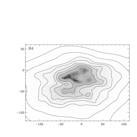
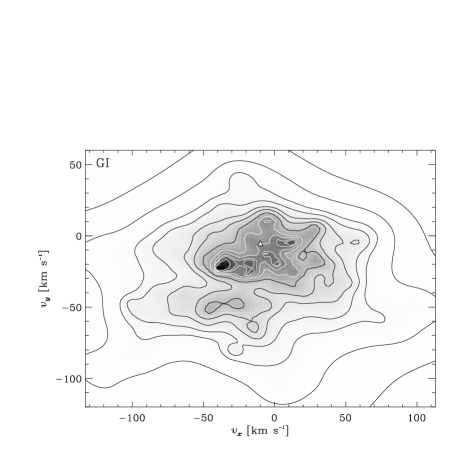
Figure 3: The distributions in $v_{x}$ (towards the Galactic center) and $v_{y}$ (in direction of Galactic rotation): projection of $f(\mbox{\boldmath$v$})$ obtained as MPLE for the sets listed in Table 1. Gray scales are linear and the contours contain, from inside outwards, 2, 6, 12, 21, 33, 50, 68, 80, 90, 95, 99, and 99.9 percent of all stars, i.e. half the stars are within the innermost dark contour. The origin is at the solar velocity, while the velocity derived for the LSR in paper I is indicated by a triangle. Note that the smoothing is optimal for the full sample (AL) only, while the results for the subsets are under-smoothed. However, since the subsets are distinct, any feature common to more than one of them is likely to be real.

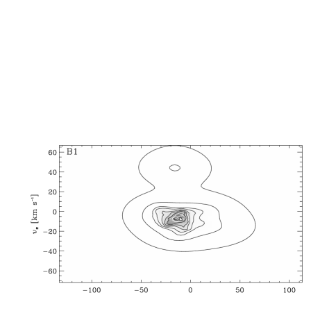
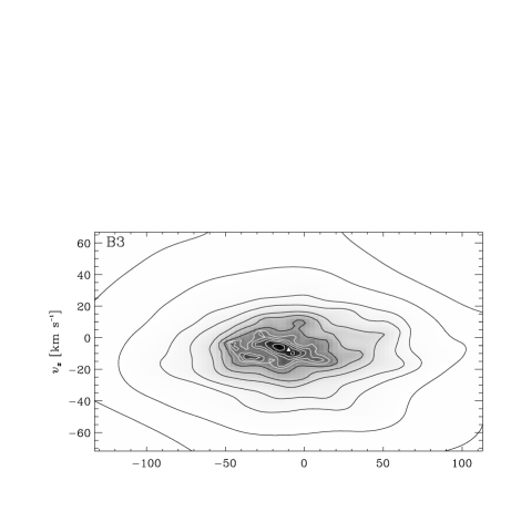
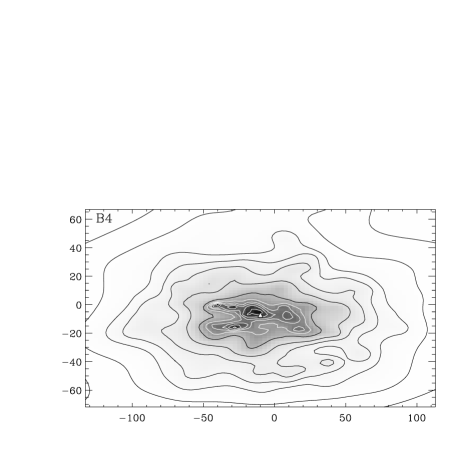
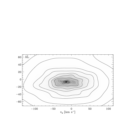
Figure 4: The distributions in $v_{x}$ (towards the Galactic center) and $v_{z}$ (towards the NGP). See Fig. 3 for the contour levels, etc.

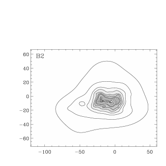
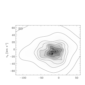
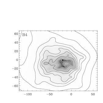
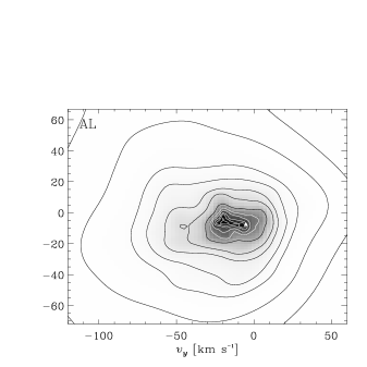
Figure 5: The distributions in $v_{y}$ (in direction of Galactic rotation) and $v_{z}$ (towards the NGP). See Fig. 3 for the contour levels, etc.

For the six sets of Table 1, Figures 3, 4, and 5 show the projections of the estimated $f(\mbox{\boldmath$v$})$ onto the $v_{x}v_{y}$, $v_{x}v_{z}$, and $v_{y}v_{z}$ plane, respectively.

Table 2: Features in the inferred velocity distributions

No.	$v_{x}$	$v_{y}$	$v_{z}$	B1	B2	B3	B4	GI		moving group
1	$-12$	$-22$	$-7$	$\bullet$	$\bullet$	$\bullet$	$\bullet$	$\circ$		Pleiades
2	$-40$	$-20$	$0$		$\bullet$	$\bullet$	$\bullet$	$\bullet$		Hyades
3	$9$	$3$		$\bullet$	$\bullet$	$\bullet$	$\bullet$	$\bullet$		Sirius & UMa
4	$-10$	$-5$	$-8$	$\bullet$	$\bullet$	$\bullet$	$\bullet$			Coma Berenices
5	$-25$	$-10$	$-15$		$\bullet$	$\bullet$	$\bullet$	$\circ$		NGC 1901
6	$20$	$-20$					$\bullet$	$\bullet$
7	$15$	$-60$					$\bullet$	$\circ$		HR1614
8	$-40$	$-50$			$\bullet$	$\bullet$	$\bullet$	$\bullet$
9	$-25$	$-50$				$\circ$	$\bullet$	$\bullet$
10	$0$	$-110$		$\bullet$		$\circ$	$\circ$	$\circ$		Arcturus
11	$-70$	$-10$				$\circ$	$\circ$	$\circ$
12	$-70$	$-50$				$\circ$	$\circ$	$\bullet$
13	$50$	$0$				$\circ$	$\bullet$	$\circ$
14	$50$	$-25$				$\circ$	$\bullet$	$\circ$

Velocities are approximate ($v_{x}$ is $-U$ in Eggen’s papers); if $v_{z}$ is missing it cannot be determined. $\bullet$ and $\circ$ denote, respectively, clear or vague visibility in the corresponding subsample. The list of associated moving groups is presumably incomplete.

The most conspicuous characteristic of the inferred velocity distributions are several strong maxima and many minor wiggles most apparent in the planar motions (Fig. 3). These features are less clear but still significant in the sample AL, for which optimal smoothing has been used. Almost all of these major and minor maxima and even some of the wiggles can be identified with one of Eggen’s (1965, 1995, 1996) moving groups. Table 2 lists the positions of 14 such features in Figures 3 to 5, together with the name of an associated moving group, where one could be found in the literature. (Some of the associations might well be wrong, for instance, Eggen gives an age of 10 Gyr for the Arcturus group, much more than any star possibly in B1.) The most prominent of these features (i.e. the first 4-5 in that table) have also been found by other groups from analysis of HIPPARCOS data, e.g. Figueras et al. (1997) using HIPPARCOS data in conjunction with radial velocities for young B5-F5 stars, and Chereul et al. (1997) using a convergent-point method (see footnote 1) for 3000 A stars. The distribution of these maxima is skewed in the $v_{x}v_{y}$ plane (but not in the other two principal planes), which in turn is responsible for the tilt in the velocity ellipsoid (vertex deviation) derived in paper I.

As one moves through the sequence B1 to B4, i.e. considers ever redder and hence on average older main-sequence stars, the following can be noticed.

• The relative number of stars in the maxima diminishes. While roughly half of the stars in subsamples B1 and B2 are associated with one of the features, in B4 over $\sim 3/4$ cent are in a smooth background distribution.

• The number of features increases. This means that some of the moving groups are old and enter the red subsamples only, whereas young clusters have stars of all colors.

• Moving groups that are present only in the red subsamples are predominantly at large negative azimuthal velocities. Thus there is a correlation in the sense that the older a moving group is, the smaller is its (local) rotational velocity around the Galaxy. Similarly, most features at small or positive $v_{y}$ decrease in amplitude as one moves to redder samples.

• The width of the distribution of moving groups clearly increases in $(v_{x},v_{y})$ but much less so in $v_{z}$. Together with (3) this means that the distribution of moving groups obeys an asymmetric drift relation.

• The width of individual maxima increases (at least for the four most prominent ones).

• From B2 to B4, the extent of the outermost two contours (containing 99 and 99.9 per cent of the stars) increases by a factor of about two in $v_{x}$ and $v_{y}$ and about three in $v_{z}$, while the center is shifted to more negative $v_{y}$, reflecting the asymmetric drift.

• From B2 to B4, the axis ratio of the outer contours changes from about 1:0.6:0.35 to 1:0.6:0.5. A similar change, however, is also visible in each individual subsample when one moves from inside (small $v$) outwards.

With respect to all these points, subsample GI of non-main-sequence stars most closely resembles sample B4 of main-sequence stars redder than $\bv=0.6\mbox{\,{\rm mag}}$.

It should be noted that, in contrast to the projections onto the $v_{x}v_{y}$ plane, most features apparent in $v_{z}$ seem not be real (they do not occur in more than one distinct subsample). In fact, they all disappear when optimal smoothing is applied (not shown) as is the case for sample AL, with the remarkable exception of the double peaked $f(v_{z})$ at $(v_{x},v_{y})\approx(-30,-20)$ in B4.

5 MOVING GROUPS AND
STELLAR STREAMS

About half of the stars in the blue color bins B1 and B2 (with $\bv\leq 0.4\mbox{\,{\rm mag}}$) are associated with moving groups, but the same holds for a considerable fraction (up to $\sim 25$ per cent) of main-sequence stars in the red color bins B3 and B4, even red-ward of Parenago’s discontinuity at $\bv\approx 0.61\mbox{\,{\rm mag}}$ (paper I), where no disk star has yet left the main sequence. This means that many of the moving groups, in particular the less prominent ones, must be made of stars older than 2-8 Gyr, the ages of the oldest stars possibly in samples B2 and B3, respectively.

5.1 The Shape of Moving Groups
in Velocity Space

According to the standard picture of these phenomena, stars form in clusters each of which is initially confined to a small volume in phase-space. Over time these dissolve, such that the old stellar population obeys a smooth distribution both in configuration and velocity space. While the mechanisms driving the evolution and dissolution of the initially bound cluster have been studied in some detail ([Terlevich 1987]), little is known about the subsequent evolution. Once the cluster becomes unbound, its stars will have slightly different orbits and hence different frequencies, such that they will phase-mix. A cluster with initial velocity dispersion $\sigma_{0}$ will be dispersed over all azimuths in a time of $2\pi R/\sigma_{0}$ ($\sim 5\,$Gyr for $R=R_{0}$ and $\sigma_{0}\approx 10\mbox{$\,{\rm km}\,{\rm s}^{-1}$}$). Since, at any fixed azimuth one expects only stars with identical azimuthal frequency, i.e. identical angular momentum, such a stellar stream is expected to manifest itself as a clump in $f(\mbox{\boldmath$v$})$ that is narrow in $v_{y}$ but has size $\gtrsim\sigma_{0}$ in $(v_{x},v_{z})$ ([Woolley 1961]). Although measurement uncertainties and noise tend to sphericalize these clumps, it is somewhat surprising, that only a few of the features in Figure 3 are elongated in this sense. However, one also expects that scattering with perturbers, like giant molecular clouds or spiral arms, will randomly change the stellar orbits and hence spread the stream deleting the correlations in velocities. On the other hand, as has long been known, the moving groups, except the very young ones, are almost indistinguishable in $v_{z}$. Presumably, this can be attributed to phase-mixing which is more efficient than for the horizontal motions, because, for any realistic disk-profile, the vertical frequency is a strong function of vertical energy, and the dynamical time is shorter by about a factor of two.

5.2 Moving Groups on Eccentric Orbits

Thus, it appears natural that there is much more structure in $(v_{x},v_{y})$ than there is in $v_{z}$, however, the character of this structure is very interesting. In particular, the fact that the distribution of moving groups obeys an asymmetric drift relation (points 3 & 4 in Section 4.2), similar to the smooth background: the older groups are more wide spread in $v$ and lag w.r.t. the LSR, i.e. they are on non-circular orbits. For stars in the smooth background these relations arise because scattering processes increase the velocity dispersion with age, and because much more stars visit us from inside the solar circle than from outside. The latter certainly also holds for the moving groups and causes the lag. However, scattering processes would destroy and disperse an existing moving group rather than shifting it to another orbit. The question therefore arises, how did the old moving groups get on their eccentric orbits?

Even tough one could imaging a scenario where the moving groups have been born onto these orbits – for instance, by star formation in the molecular gas ring at $\sim 4\mbox{$\,{\rm kpc}$}$, where the Galactic bar significantly distorts the axisymmetry – this seems unlikely in view of the facts that phase-mixing should have spread these moving groups in $v_{x}$ and that the apparently young moving groups are indeed on near-circular orbits. Alternatively, the moving groups could have been transformed to more eccentric orbits. This would naturally account for the age-dependence of the eccentricity. Since a moving group is a rather fragile object, any non-axisymmetric force field responsible for such a process must be smooth, both in space (long wavelength) and time (low frequency). While a triaxial halo or the Magellanic clouds might play a role in such an process, the most obvious candidate is the Galactic bar. Actually, almost all the apparently older moving groups have negative $v_{y}$, and thus low $L_{z}$, they are near the apocenters of their orbits, which probe a large range of radii and come near to the bar.

A plausible mechanism that is able to shift moving groups to eccentric orbits has been described by Sridhar & Touma (1996). Applied to our problem it works as follows. If the otherwise axisymmetric Galaxy is perturbed by some non-axisymmetric component, its phase-space structure will change, the degeneracy will be broken, and resonant islands will occur, regions in phase-space surrounding resonant orbits. The orbits in these islands are near-resonant and oscillate around their resonant parent orbit. When the Galaxy slowly evolves, for instance, when the Galactic bar slows down and strengthens, these resonant islands sweep through phase-space, and stars trapped in them will be shifted to different orbits – an effect also known from the dynamics of the solar system.

Actually, there is a clear pointer to the involvement of resonances in the motion of nearby stars: the recent re-determination of Oort’s constants from HIPPARCOS Cepheids by Feast & Whitelock (1997) gives (in $\,{\rm km}\,{\rm s}^{-1}\,{\rm kpc}^{-1}$) $\Omega=A-B=27.2\pm 0.9$, $\kappa=2\sqrt{B^{2}-AB}=36.7\pm 1.6$, and $\Omega\,:\,\kappa=2.97\pm 0.07\,:\,4$. That is very precisely a 3:4 resonance between the azimuthal and radial orbital frequency, a ratio which appears naturally in a slightly declining circular-speed curve, e.g. of the form $v_{c}\propto R^{-1/9}$. 3:4 resonant orbits complete four radial oscillations in the same time they rotate three times around the Galactic center; during this time they visit any given azimuth with three different velocities. In this respect it is intriguing that the stars in B1, which are at most two orbital rotation periods old, show just two distinct peaks in their velocity distribution.

Currently, the only model that aims to explain the structure in $(v_{x},v_{y})$ does in fact invoke a resonance, although, not the one mentioned above. This model is due to Kalnajs (1991), who starts from the observation of just two major maxima (at the Sirius and Hyades peaks), and locates the Sun at the outer Lindblad resonance (OLR) of the Galactic bar. The closed orbits inside and outside the OLR are elongated, respectively, perpendicular and parallel to the bar. At some azimuths these differently orientated orbits cross and naturally create a double-peaked distribution in $(v_{x},v_{y})$. This model gives pattern speed and projection angle of the Galactic bar in rough agreement with other methods, but does not account for the asymmetric drift relation amongst moving groups.

6 EVIDENCE FOR THE STELLAR WARP

In Figure 5, in all samples except B1 and best visible in GI and AL, the few outermost contours are somewhat skewed in the sense that at positive $v_{y}$ more stars are moving upwards w.r.t. the LSR than downwards. This is nicely illustrated in Figure 6, where the mean vertical motion due to $f(\mbox{\boldmath$v$})$ inferred from the full sample is plotted versus $v_{y}$. While $\bar{v}_{z}$ is roughly constant at the LSR value of $-7\mbox{$\,{\rm km}\,{\rm s}^{-1}$}$ for $v_{y}\la 10\mbox{$\,{\rm km}\,{\rm s}^{-1}$}$ (the bends are presumably due to the moving groups), it clearly curves upwards for $v_{y}\ga 10\mbox{$\,{\rm km}\,{\rm s}^{-1}$}$ (this is not an ordinary tilt, which would produce a straight line in this diagram).

Figure 6: The mean vertical motion, $\bar{v}_{z}$, measured from sample AL as a function of of $v_{y}$. The errors bars show 1 $\sigma$ errors due to Poisson noise; however, adjacent points are not independent but coupled by the smoothing. The triangle indicates the velocity of the LSR, and the lines are derived from models for the Galactic warp, see text.

This effect can be nicely explained by the Galactic warp. The Sun roughly lies at the inner edge of the warp on the line of nodes such that nearby stars that participate in the warp have $v_{z}>0$. For such stars to enter our very local sample, they must be near the pericenter of their orbits, and hence have $v_{y}>0$. To be more quantitative, let me model the height $z$ of the Galactic disk as a function of galacto-centric distance $R$ and azimuth $\varphi$ (with $\varphi=0$ at the Sun) by

$$z=h(R)\,\sin(\varphi+\Omega_{p}t),$$ (38)

where $\Omega_{p}$ is the pattern speed with $\Omega_{p}>0$ meaning a retrograde motion w.r.t. the stellar orbits, as expected from almost all theoretical warp models. I take the height function

$$h(R)=(R-r_{w})^{2}/r_{h},$$ (39)

where $r_{w}$ is the edge of the flat part of the disk and $r_{h}$ then sets the amplitude of the warp. For a star with guiding center $R$, we expect from the conservation of angular momentum

$$v_{y}={R^{2}\over R_{0}}\Omega(R)-R_{0}\Omega(R_{0})-v_{\odot y}$$ (40)

and a mean vertical motion of $\bar{v}_{z}=v_{z}(R)-v_{z}(R_{0})-v_{\odot z}$ with (using $\varphi=\Omega t$)

$$v_{z}(R)={{\rm d}z\over{\rm d}t}=\big{(}\Omega(R)+\Omega_{p}\big{)}\,h(R)\,\cos\varphi,$$ (41)

where $\Omega(R)$ is the circular frequency and $\mbox{\boldmath$v$}_{\odot}=($10.0, 5.2, 7.2)$\,{\rm km}\,{\rm s}^{-1}$ is the solar motion w.r.t. the LSR as derived in paper I. The lines in Figure 6 have been computed assuming a slightly falling rotation curve of the form $R\Omega\propto R^{-1/9}$, $R_{0}=8\mbox{$\,{\rm kpc}$}$, and $\Omega(R_{0})=27.2\mbox{$\,{\rm km}\,{\rm s}^{-1}\,{\rm kpc}^{-1}$}$ ([Feast & Whitelock 1997]). The dashed line is for a model with $r_{w}=6.5\mbox{$\,{\rm kpc}$}$, $r_{h}=15\mbox{$\,{\rm kpc}$}$, given for the H i by Diplas & Savage (1990), and $\Omega_{p}=0$. Note that, for the rotation curve adopted, $v_{y}=40\mbox{$\,{\rm km}\,{\rm s}^{-1}$}$ originates from a guiding center of $R=10\mbox{$\,{\rm kpc}$}$. Clearly, this model does not fit the data and non-zero $\Omega_{p}$ would make it even worse. The obvious reason for this failure is the fact that the modeled warp starts well inside the solar circle, and predicts a strong effect already near the LSR. The full (almost indistinguishable) lines show four models with an inner edge of the warp of $r_{w}=R_{0}$, various pattern speeds in the range $0\leq\Omega_{p}\leq 30\mbox{$\,{\rm km}\,{\rm s}^{-1}\,{\rm kpc}^{-1}$}$, and with $r_{h}$ chosen such that the pattern speed and the amplitude $z_{10}$ of the warp at $R=10\mbox{$\,{\rm kpc}$}$ obey

$${\Omega_{p}\over\mbox{$\,{\rm km}\,{\rm s}^{-1}\,{\rm kpc}^{-1}$}}={4-6(z_{10}/\mbox{$\,{\rm kpc}$})\over 0.3(z_{10}/\mbox{$\,{\rm kpc}$})}.$$ (42)

These models give good descriptions of the data at all valid points. Thus, to explain the observed effect, the Galactic warp must not start inside the solar circle. On the other hand, only a combination of the amplitude of the warp and its pattern speed is constraint by the data. With the above parameters for the Galactic rotation curve and $R_{0}$, the H i data of Burton (1992) yield a warp amplitude $z_{10}$ of 0.3 to 0.4$\,{\rm kpc}$, resulting in $\Omega_{p}$ of $13$ to $25\mbox{$\,{\rm km}\,{\rm s}^{-1}\,{\rm kpc}^{-1}$}$. The infrared data taken by DIRBE suggest that the stellar warp might have half that amplitude ([Freudenreich et al. 1994]), in which case $\Omega_{p}$ must be larger.

7 CONCLUSION

I have analyzed a kinematically unbiased sample of more than 14 000 nearby stars with positions, parallaxes, and proper motions known accurately from ESA’s astrometric mission ‘HIPPARCOS’. From the same sample, we have re-determined in paper I ([Dehnen & Binney 1998b]), as a function of color, the mean velocity and velocity dispersion for main-sequence stars in the solar neighborhood. In this paper, the velocity distribution $f(\mbox{\boldmath$v$})$ itself, rather than its first two moments, has been inferred.

Although radial velocities are available for a fraction of these stars, they could not be used because they are predominantly known for high-velocity stars and would inevitably introduce a kinematic bias. Without knowledge of radial velocities, the inference of $f(\mbox{\boldmath$v$})$ is formally equivalent to a deprojection and an example of an astronomical inverse problem. A maximum-penalized-likelihood (MPL) technique for the recovery of $f(\mbox{\boldmath$v$})$ from the positions and tangential velocities of individual stars has been developed.

Poisson noise completely dominates the errors, and the number of stars is too small to recover the three-dimensional distribution with useful resolution, but any two-dimensional projection can be determined with reasonable accuracy. The resulting distributions of nearby stars in $(v_{x},v_{y})$, $(v_{x},v_{z})$, and $(v_{y},v_{z})$ are shown in Figures 3, 4, and 5, respectively. ($v_{x}$, $v_{y}$, and $v_{z}$ denote the velocity components in the directions of the Galactic center, Galactic rotation, and the north Galactic pole, respectively). The sample has been split into four color bins (B1 to B4) of main-sequence stars and non-main-sequence stars (GI), mainly giants. Additionally, the sample has been analyzed as a whole (AL).

7.1 The Smooth Background

At large velocities and/or redder color most stars are in a smooth and approximately ellipsoidal background distribution. The axis ratio of this background distribution increases from early to late stellar types. The increase is stronger in $v_{z}$ than it is in the horizontal motions, implying that the vertical heating becomes relatively more important for on average older and hence dynamically hotter stellar populations. This is expected if scattering by spiral structure is important, since for stars with epicycle diameters larger than the inter-arm separation, this process becomes inefficient ([Jenkins 1992]). From Figure 4, sample AL, I estimate that the effect sets in at $|v_{x}|$ of $\sim 60\mbox{$\,{\rm km}\,{\rm s}^{-1}$}$ corresponding to an epicycle diameter of $\sim 3\mbox{$\,{\rm kpc}$}$ (with $\kappa=36.7\mbox{$\,{\rm km}\,{\rm s}^{-1}\,{\rm kpc}^{-1}$}$).

The background distribution also shows nicely the asymmetric drift relation: for ever later stellar types, the outermost contours in Figs. 3 to 5 are larger and their centroid is shifted more and more to negative $v_{y}$. These contours appear to be aligned with the $v_{x}$ axis (radial) but slightly skewed w.r.t. the $v_{y}$ and $v_{z}$ axes. The latter can nicely be explained by the Galactic warp: orbits participating in it move upwards and must have $v_{y}>0$ in order to enter our local sample. A more quantitative analysis reveals that the warp must not start within the solar circle and has pattern speed $\gtrsim 13\mbox{$\,{\rm km}\,{\rm s}^{-1}\,{\rm kpc}^{-1}$}$ with sense of rotation opposite to the stellar orbits, as is theoretically expected.

7.2 The Moving Groups

Apart from the smooth background, $f(\mbox{\boldmath$v$})$ shows a lot of structure, in particular in the horizontal motions (Fig. 3): there are various major and minor maxima and smaller features that seem to be real, in as much as they appear in more than one of the distinct subsamples. A peak in $f(\mbox{\boldmath$v$})$ corresponds to a group of stars moving with the same velocity, and indeed, many maxima correspond to one of the moving groups already identified by Kapteyn (1905) and later studied by Eggen (e.g. 1965). The fact that these moving groups are much less visible in $v_{z}$ can be attributed to phase-mixing. What seems to be surprising, however, is that the distribution of moving groups obeys an asymmetric drift relation, similar to the smooth background: the apparently older groups (as judged from their minimum color) are more wide spread in $(v_{x},v_{y})$ and lag w.r.t. the LSR, i.e. they are on non-circular orbits. A possible explanation for a moving groups on such an eccentric orbits is as follows. A cluster of stars is born onto a near-circular orbit similar to those of the molecular gas. The stars might then be trapped into a resonance with a non-axisymmetric force field like that of the Galactic bar. If this force field slowly evolves, the resonances are shifted in orbit space and with them the stars trapped. This mechanism is well known from solar system dynamics and has recently been proposed to explain the thick disk ([Sridhar & Touma 1996]).

To interpret properly the results of this paper, i.e. to answer the question why $f(\mbox{\boldmath$v$})$ shows the observed structure, we clearly need a better understanding of the processes potentially involved in the dynamical evolution of the solar neighborhood, in particular, with regard to the effect of orbital resonances. These processes include (i) phase-mixing; (ii) scattering by small random perturbations of the Galactic force field, like giant molecular clouds and temporary spiral arms; (iii) interactions with large transient perturbers, for example, merging satellites of the Milky Way, such as the Saggritarius dwarf galaxy; and (iv) forcing by regular non-axisymmetric components of the gravitational potential, like the central bar, a long-living spiral pattern, a triaxial halo, or the Magellanic clouds. For the processes (i), (iii), and (iv), resonances in the stellar motions and/or between these and the motions of the perturbing agents are likely to be important and may lead to a behavior completely different from that of the non-resonant case.

References

- [Binney et al. 1997] Binney J.J., Dehnen W., Houk N., Murray C.A., Penston M.J., 1997, ESA SP-402, Hipparcos-Venice’97, p. 473
- [Binney & Tremaine 1987] Binney J.J., Tremaine S., 1987, Galactic Dynamics. Princeton Univ. Press, Princeton
- [Bressan et al. 1993] Bressan A., Fagotto F., Bertelli G., Chiosi C., 1993, A&AS, 100, 647
- [Burton 1992] Burton W.B., 1992, in Pfenniger D., Bartholdi P., eds., The Galactic Interstellar Medium, Springer, New York, p. 134
- [Chereul et al. 1997] Chereul E., Crézé M., Bienaymé O., 1997, ESA SP-402, Hipparcos-Venice’97, p. 545
- [Dehnen & Binney 1998a] Dehnen W., Binney J.J., 1998a, MNRAS, 294, 429
- [Dehnen & Binney 1998b] Dehnen W., Binney J.J., 1998b, MNRAS in press (paper I, astro-ph/9710077)
- [Diplas & Savage 1990] Diplas A., Savage B.D., 1990, ApJ, 277, 126
- [Eggen 1965] Eggen O.I., 1965, in Blaauw A.A., Schmidt M., eds., Stars and Stellar Systems V., Univ. of Chicago Press, p. 111
- [Eggen 1995] Eggen O.I., 1995, AJ, 111, 1615
- [Eggen 1996] Eggen O.I., 1996, AJ, 112, 1595
- [ESA 1997] ESA, 1997, The Hipparcos and Tycho Catalogues, ESA SP-1200
- [Feast & Whitelock 1997] Feast M.W., Whitelock P.A., 1997, MNRAS, 291, 683
- [Figueras et al. 1997] Figueras F. et al., 1997, ESA SP-402, Hipparcos-Venice’97, p. 519
- [Jenkins 1992] Jenkins A., 1992, MNRAS, 257, 620
- [Freudenreich et al. 1994] Freudenreich H.T. et al., 1994, ApJ, 429, L69
- [Kalnajs 1991] Kalnajs A.J., 1991, in Sundelius B., ed., Dynamics of Disc Galaxies, Göteborg, Sweden, p. 323
- [Kapteyn 1905] Kapteyn J.C., 1905, Brit. Ass. Rep., p. 257
- [Lucy 1974] Lucy L.B., 1974, AJ, 79, 745
- [Lucy 1994] Lucy L.B., 1994, A&A, 289, 983
- [Press et al.1992] Press W.H., Teukolsky S.A., Vetterling W.T., Flannery B.P., 1992, Numerical Recipes. Cambridge Univ. Press, Cambridge
- [Richardson 1972] Richardson W.H., 1972, J. Opt. Soc. Am., 62, 55
- [Schwarzschild 1908] Schwarzschild K., 1908, Nachr. Kgl. Ges. d. Wissenschaften, Göttingen, 191
- [Silverman 1982] Silverman B.W., 1982, Annals of Statistics, 10, 795
- [Silverman 1986] Silverman B.W., 1986, Density Estimation, Chapman & Hall, London
- [Sridhar & Touma 1996] Sridhar S., Toume J., 1996, MNRAS, 279, 1263
- [Terlevich 1987] Terlevich E., 1987, MNRAS, 224, 193
- [Woolley 1961] Woolley R.v.d.R., 1961, Obs, 81, 203