The ESO Slice Project [ESP] galaxy redshift survey:

Abstract

The issue of the approximate isotropy and homogeneity of the observable universe is one of the major topics in modern Cosmology: the common use of the Friedmann–Robertson–Walker [FWR] metric relies on these assumptions. Therefore, results conflicting with the “canonical” picture would be of the utmost importance. In a number of recent papers it has been suggested that strong evidence of a fractal distribution with dimension $D\simeq 2$ exists in several samples, including Abell clusters [ACO] and galaxies from the ESO Slice Project redshift survey [ESP].

Here we report the results of an independent analysis of the radial density run, $N(<R)\propto R^{D}$, of the ESP and ACO data.

For the ESP data the situation is such that the explored volume, albeit reasonably deep, is still influenced by the presence of large structures. Moreover, the depth of the ESP survey ($z\la 0.2$) is such to cause noticeable effects according to different choices of k-corrections, and this adds some additional uncertainty in the results. However, we find that for a variety of volume limited samples the dimensionality of the ESP sample is $D\approx 3$, and the value $D=2$ is always excluded at the level of at least five (bootstrap) standard deviations. The only way in which we reproduce $D\approx 2$ is by both unphysically ignoring the galaxy k–correction and using Euclidean rather than FRW cosmological distances.

In the cluster case the problems related to the choice of metrics and k–correction are much lessened, and we find that ACO clusters have $D_{ACO}=3.07\pm 0.18$ and $D_{ACO}=2.93\pm 0.15$ for richness class $\hbox{$\cal R$}\geq 1$ and $\hbox{$\cal R$}\geq 0$, respectively. Therefore $D=2$ is excluded with high significance also for the cluster data.

1 Introduction

Recently Pietronero and collaborators [hereafter P&C] (Pietronero et al. Pprinc (1997), Sylos Labini et al. SLGMP (1996), Baryshev et al. SLPvistas (1994)) argued that a large number of samples give strong evidence that the distribution of clusters and galaxies is a simple fractal of dimension $D\simeq 2$ on scales of several hundreds of Mpc, quite different from the “canonical” value of $D=3$.

This is an important claim because of its far reaching implications, and this issue, which dates back to the beginning of the century (Charlier, 1908, see Peebles peebles (1993)), can be properly addressed with long and careful analyses which, however, demand much deeper and better samples than those presently available in order to be able to explore an adequate range of scales (see e.g. Mc Cauley McCauley97 (1997), Hamburger et al. Hamburger+96 (1996)). While 2D constraints come from fluctuations in cosmic backgrounds (see e.g. Peebles 1993), historically much work on this subject has been done for decades in analyzing galaxy counts which, in a non evolving Euclidean Universe, should follow $N(m)\propto 10^{0.6m}$. Indeed, this behaviour has been observed in an intermediate magnitude range, $m\approx 15\div 17$, (see e.g. Sandage sandage (1995)). However, on the bright side one has to deal with magnitude errors given from saturation of photographic plates and/or the relatively small volumes sampled which also reflect in uncertainties in locally the derived space galaxy density (cf Loveday et al. SAPM (1992), Zucca et al. 1997, Maddox maddox (1997)), while on the faint side cosmological curvature and evolutionary effects become dominant and difficult to disentangle (Koo & Kron kookron (1992), Ellis ellis (1997)). Therefore one really needs redshift information in order to avoid effects of time–space projections.

In this paper we limit ourselves to an independent check on two of the samples discussed by P&C, the ESP galaxies (Vettolani et al. paolo+97 (1997)) and the ACO clusters (Abell, Corwin & Olowin ACO (1989)), without touching upon the very general issue of a possible fractal distribution of the matter in the universe and its consequences: the interested reader can consult Peebles (peebles (1993)), Coleman & Pietronero (CP (1992)), Stoeger et al. (SEH (1987)), Ehlers & Rindler (ER (1987)), Szalay & Schramm (SS (1985)), Luo & Schramm (LS (1992)), Mc Cauley (McCauley97 (1997)), Buchert (Buchert97 (1997)), Guzzo (gigi97 (1997)) and references therein.

However, if the evidence were present in the data at the highly significant level claimed by P&C, the simple analysis presented here should be more than adequate in confirming the $D=2$ claims.

In section 1 we present the formalism, in section 2 the results from ESP galaxies, in section 3 the results from the ACO clusters, and finally in section 4 the conclusions.

2 Method

In a previous discussion (Scaramella et al. io+91 (1991)) on the origin of the Local Group velocity with respect to the Cosmic Microwave Background frame, it was pointed out the relevance of the depth’s behaviour of clusters’ “monopole” and “dipole” with respect to the issue of approach to homogeneity of the matter distribution (see Sylos Labini Sylos94 (1994) for contrasting views).

The method, adopted also by P&C, is very simple: basically, after selecting a volume limited sample of objects, one considers the quantity

$$N(<R)=\int_{0}^{R}dr\,\sum_{i}\delta(r-r_{i})$$ (1)

where $r_{i}$ are the radial distances of the objects in the sample and $\delta$ is the Dirac distribution.

Now, for a simple fractal of dimension $D$ one has

$$\langle N(<R)\rangle=const\cdot R^{D}$$ (2)

One should notice an important difference between the two above expressions: while Eq. 1 refers to a single point (the origin), Eq. 2 refers to a statistical property of the sample, i.e. is obtained by averaging on all points of the sample (for which several methods have been discussed in the literature). However, also according to P&C, for samples with an adequate number of objects even with Eq. 1 one should recover, after some initial fluctuations (Sylos Labini et al. SLGMP (1996)), the “correct” dependence on distance of Eq. 2 for a fractal distribution, that is $N(<R)=\int_{0}^{R}dr\,\sum_{i}\delta(r-r_{i})\;\propto\;R^{D}$. Therefore P&C considered an expression equivalent to Eq. 1, the integral density $N(<R)/R^{3}\propto R^{D-3}$, and derived the value $D\simeq 2$ from preliminary ESP data up to depths of several hundreds of Mpc.

3 ESP survey

The ESP final sample of galaxies (Vettolani et al. 1997, 1998), limited in apparent magnitude in the $b_{J}$ band ($b_{J}\leq 19.4$), is highly complete in the fraction of measured redshifts ($\sim 85\%$). Despite this fact, its analysis in terms of volume–limited subsamples is not entirely trivial.

Figure 1: Limiting distances for ESP volume limited samples with different assumptions for metric and k–correction.

The results are somewhat dependent on the assumptions on the cosmological parameters, and some uncertainty is induced by the statistical error on the observed magnitudes (r.m.s. of $\simeq 0.2$ mags) and the uncertainties in the adopted k-corrections.

Figure 2: Cumulative depth distribution of the number of ESP galaxies for three volume limited subsamples of case (i), cosmological distance and average k–correction. The value of slope fitted for $R\geq 300$ Mpc/h is shown close to the relative line. The total number of galaxies in each subsample is given in the legend.

In our analysis we will use the standard formula to derive the absolute magnitude:

$$M_{b_{J}}\;=\;b_{J}-5\cdot\left\{5+\log[r_{lum}(z)]+\log(h)\right\}-k(z)$$ (3)

where $k$ is the k–correction term (discussed below), $r_{lum}$ is the luminosity distance in Mpc (we assume $H_{0}=100$ $h\,$$km\,$ $s^{-1}\,$ $Mpc^{-1}$ and $\Omega_{0}=1,\Lambda=0$); henceforth we will drop the _J subscript from the magnitudes.

We will consider ESP volume limited subsamples obtained with three cuts in absolute luminosity, namely $M_{b_{lim}}=-19.5$, $-20.0$, $-20.5$. These limits span increasingly deeper volumes with decreasing statistics. Obviously the limiting distances of the volume limited subsamples are function of the adopted cosmological model and k–correction. In the following we will consider comoving radial distance: $r_{com}=r_{lum}/(1+z)$. In the Euclidean case we will have $r_{com}=r_{lum}=cz/H_{0}$.

Figure 3: Cumulative depth distribution of the number of ESP galaxies for three volume limited subsamples of case (v), Euclidean distance and zero k–correction. The value of slope fitted for $R\geq 300$ Mpc/h is shown close to the relative line. The total number of galaxies in each subsample is given in the legend.

In Fig. 1 we show the limiting distances for volume–limited subsamples as a function of absolute magnitude for five different cases:

• cosmological distance and average k–correction as in Zucca et al. (zucca+97 (1997));

• cosmological distance and k–correction estimated from the spectrum of each galaxy (Fiorani & Scaramella ago+io98 (1998));

• Euclidean distance and k–correction as in case (i);

• cosmological distance and zero k–correction;

• Euclidean distance and zero k–correction.

Except for case (ii) the adopted k–correction at any given redshift is the same for all galaxies and in these cases the definition of a volume limited subsample is straightforward. In case (ii) we have to limit the depth in such a way to include all morphological types, and therefore we define the limiting distance by using $k_{lim}(z)\simeq 4.1\,z$, i.e. the k-correction appropriate for elliptical galaxies in our redshift range, $z\la 0.25$.

For the ESP sample P&C claim that the signature of $D=1.9\pm 0.2$ is seen for volume limited sub–samples at a depth greater than $300\,$ Mpc/h, which according to Sylos Labini et al. (SLGMP (1996)) is the minimum depth of statistical validity of the radial analysis for this sample.

We show in Fig. 2 the results of fitting $D$ in Eq. 2 to the three volume limited subsamples of case (i) in the range $R\geq 300$ Mpc/h. The influence of the large inhomogeneity reported in Zucca et al. (zucca+97 (1997)) is evident in all subsamples up to a depth of $R\sim 300$ Mpc/h, but after that we find no evidence for a slope $\sim 2$, as claimed by P&C.

Since the data presented in Fig. 2 are cumulative distributions, the points are not independent. Therefore in order to have an estimate of the error associated to the fitted value we applied the bootstrap method (Efron & Tbishirani bootref (1993)), which yields a measure of the internal uncertainty of the sample at hand. The bootstrap estimates from 10,000 resamplings have a Gaussian shape and yield: $D_{-19.5}=2.93\pm 0.14$ , $D_{-20}=3.08\pm 0.18$ and $D_{-20.5}=3.47\pm 0.28$. These values are all consistent with $D=3$, while for all of them $D=2$ is at more than five standard deviations. If we analyze case (ii) (cosmological distance and k–correction estimated from the spectrum of each galaxy) we obtain values in good agreement with case (i), as reported in Table 1. If we modify case (i) with the use of Euclidean distances rather than the comoving ones, we still obtain values which bracket $D=3$ (case iii).

Table 1 Values of D for volume–limited ESP subsamples
Case	Model	k–correction	M-19.5	M-20.0	M-20.5
(i)	FRW	$\langle k\rangle$	2.93	3.08	3.47
(ii)	FRW	$k_{i}$	2.79	3.06	3.23
(iii)	Euclid	$\langle k\rangle$	2.96	2.83	3.17
(iv)	FRW	$0$	2.37	2.37	2.11
(v)	Euclid	$0$	2.25	1.99	1.68

On the contrary, if we neglect the use of k–corrections, we obtain values closer to $D=2$ (case iv), or even in agreement with $D=2$ (case v: $D_{-19.5}=2.25\pm 0.10$ , $D_{-20}=1.99\pm 0.13$ and $D_{-20.5}=1.68\pm 0.26$), thus reproducing the result of P&C. The results for the last case are shown in Fig. 3. Since the effect of neglecting the k–correction term in Eq. 3 is to assign a lower intrinsic luminosity to each galaxy, the brightest subsample has only $43$ galaxies and is dominated by discreteness.

The results of the present analysis show the capital importance of the k–correction term: unless one is willing to disregard the physical effect of the redshift on the observed spectrum and intrinsic luminosity (and moreover to adopt a purely Euclidean metric), our results do not support the claims of P&C of a value $D=2$ for the ESP survey, but rather suggest the value $D\simeq 3$. It is worthwhile to stress that the k–correction is an empirical and necessary correction to the magnitude of a galaxy, and it does not depend on any interpretation of the redshift. This correction simply takes into account that at different redshifts we are looking at different regions of the galaxy spectrum.

4 Abell clusters

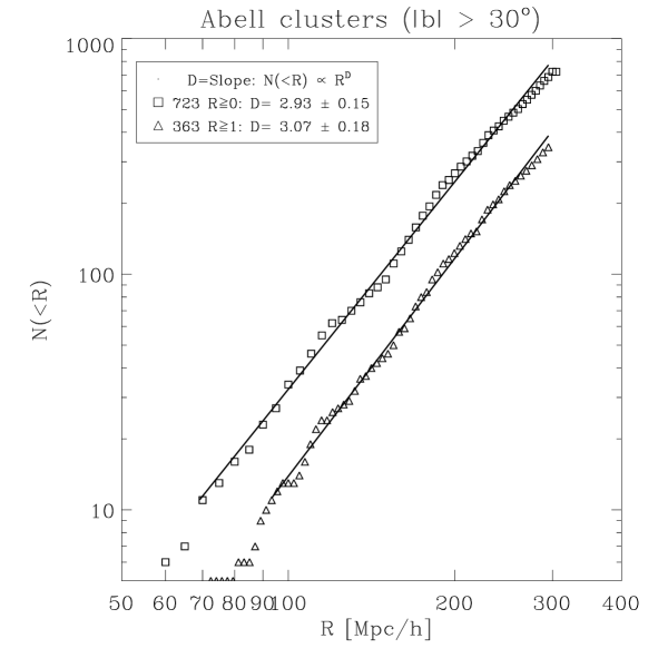
Figure 4: Cumulative depth distribution of the number of ACO clusters for volume limited subsamples.

In agreement with several analyses which appeared on the subject (see e.g. Bahcall bahcrev (1988) and reference therein), Scaramella et al. (io+90 (1990)) and Zucca et al. (zucca+93 (1993)) found that the ACO sample suffers from a significant radial incompleteness beyond a depth of $300\,$ Mpc/h. Even though the different angular selection functions and overall completeness are different for the Northern (original Abell) and the Southern sample, it has been argued (Scaramella et al. io+90 (1990)) that the radial incompleteness is not very strong within $300\,$ Mpc/h. In this case, quite differently from clustering analyses, the angular selection function should impact only on the amplitude but not on the radial behaviour of the scalar quantity $N(<R)$. We will therefore consider ACO clusters which have $|b|\geq 30^{o}$ and $R\leq 300$ Mpc/h without any correction for angular incompleteness.

We show in Fig. 4 the results of applying Eq. 2 to the combined North+South sample. Not all the clusters have measured redshift: for those for which a measure of $z$ is not available, we have used estimated $z$ from relations which have $<20\%$ of uncertainty, as reported in the papers above. We have 268 measured $z$ out of 363 for $\hbox{$\cal R$}\geq 1$ and 481 out of 723 for $\hbox{$\cal R$}\geq 0$. The clusters with estimated redshifts concentrate into the $R\ga 250$ Mpc/h region (within which there is $\sim 85\%$ of measured $z$) and can affect only the last points of Figure 4

Repeating the same fitting as done in the ESP case, and estimating similarly the errors on $D$, we obtain $D=3.07\pm 0.18$ and $D=2.93\pm 0.15$ for richness class ${\cal R}\geq 1$ and ${\cal R}\geq 0$, respectively.

We draw the conclusion that our analysis excludes $D=2$ with high levels of significance also for clusters, while it favours the canonical value $D=3$.

5 Conclusions

On the basis of the present analysis we do not find any evidence in the ESP and ACO samples for a fractal exponent $D\approx 2$ as claimed by P&C. For the ESP sample we showed that $D\approx 2$ can be obtained only by neglecting the k–correction term: in our opinion to neglect this term would be both unphysical and unjustified. Moreover, also the cluster sample, which is not significantly affected by this particular uncertainty, clearly excludes the value $D=2$.

On the contrary, we find evidence that within the errors both samples show a behaviour on large scales both consistent with and supporting the canonical value, namely $D=3$. It must be stressed that our results use direct depth information differently from indirect arguments such as scaling of angular correlation functions or fluctuations of cosmic backgrounds (see e.g. Peebles peebles (1993)).

The above conclusions suggest the need of further and more careful and sophisticated studies on the claims of a strong evidence for a fractal matter distribution from the data sets we analyzed. Also further independent checks should be done and possibly on other, better suited samples.

- (1) Abell, G.O, Corwin, H.C., & Olowin, R.P., 1989, ApJS 70, 1.
- (2) Bahcall, N., 1988, ARA&A 26, 631
- (3) Baryshev, Yu. V.,Sylos Labini, F., Montuori, M., Pietronero, L., 1994, Vistas in Astronomy, Vol. 38 part 4.
- (4) Buchert, T., 1997, astro–ph/9706214
- (5) Coleman, P.H., & Pietronero, L., 1992, PhysRep 213, 311.
- (6) Efron, B, and Tbishirani, R.J., “An Introduction to the Bootstrap”, 1993, London: Chapman & Hall .
- (7) Ehlers, J., and Rindler, W., 1987, A&A 174, 1
- (8) Ellis, R.S., 1997, ARA&A 35 389.
- (9) Fiorani, A., and Scaramella, R., 1998, in preparation.
- (10) Guzzo, L., 1997, New Astronomy 2, 517.
- (11) Guzzo, L., Iovino, A., Chincarini, G., Giovanelli R., & Haynes, M.P, 1991, ApJ 382, L5
- (12) Hamburger, D., Biham, O., & Avnir, D., 1996, cond–mat/9604123
- (13) Loveday, J., Peterson, B.A., Efstathiou, G., and Maddox, S.J., 1992, ApJ 390 338
- (14) Koo, D.C., and Kron, R.G., 1992, ARA&A 30, 616
- (15) Maddox, S.J., 1997, astro–ph/97/11015
- (16) McCauley, J.L., 1997, astro–ph/9703046
- (17) Luo, X., and Schramm, D., 1992, Science 256, 513.
- (18) Peebles, P.J.E., 1993, “Principles of Physical Cosmology”, Princeton U. Press.
- (19) Pietronero, L., Montuori, M., and Sylos Labini, F., 1997, in “Critical Dialogues in Cosmology”, N. Turok (ed.), in press.
- (20) Sandage, A.R., 1995, “The Deep Universe”, Saas-Fee advanced course 23, Springer Verlag.
- (21) Scaramella, R., Vettolani, G., & Zamorani, G., 1991, ApJ l 376, L1
- (22) Scaramella, R., Zamorani, G., Vettolani, G., & Chincarini, G., 1990, AJ 101, 342
- (23) Stoeger, W.R., Ellis, G.F.R., and Hellaby, 1987, MNRAS 226, 373
- (24) Sylos Labini, 1994, ApJ 433, 464
- (25) Sylos Labini, F., Gabrielli, A., Montuori, M., and Pietronero, L., 1996, Physica, A226, 195
- (26) Szalay, A., and Schramm, D, 1985, Nat 314, 718
- (27) Vettolani, G., et al, 1997, A&A 325, 954.
- (28) Vettolani, G., et al, 1998, A&AS in press.
- (29) Zucca, E., Zamorani, G., Scaramella, R., & Vettolani, G., 1993, ApJ 407, 470
- (30) Zucca, E., et al, 1997, A&A 326, 477