Using the DIRBE/IRAS All-Sky Reddening Map To Select Low-Reddening Windows Near the Galactic Plane

Abstract

Recently Schlegel, Finkbeiner & Davis published an all-sky reddening map based on the COBE/DIRBE and IRAS/ISSA infrared sky surveys. Using the reddening map of Baade’s Window and sample of 19 low-latitude ($|b|<5\deg$) Galactic globular clusters I find that the DIRBE/IRAS reddening map overestimates $E(B-V)$ at low galactic latitudes by a factor of $\sim 1.35$. I also demonstrate the usefulness of this high resolution map for selecting low-reddening windows near the Galactic plane.

1 INTRODUCTION

We live in a dusty Universe (Hoover 1998, private communication), and correcting for the dust extinction and reddening affects almost all aspects of optical astronomy. For us, observing from within the Milky Way, it is of crucial importance to know how much Galactic dust there is towards various objects. Burstein & Hailes (1982; hereafter: BH) constructed an all-sky reddening map, used extensively by the astronomical community. Recently, Schlegel, Finkbeiner & Davis (1998; hereafter: SFD) published a new all-sky reddening map, based on the COBE/DIRBE and IRAS/ISSA maps. This map is intended to supersede the BH map in both the accuracy and the spatial resolution ($6.1^{\prime}$). Also, unlike the BH map, which presented the $E(B-V)$ values only for the $|b|>10\deg$ regions, the SFD map extends all the way to the Galactic plane.

There are many instances when one would like to be able to identify low-reddening regions near the Galactic plane. As an example, the expected microlensing optical depth increases strongly towards the Galactic center (e.g. Stanek et al. 1997, their Figure 12). In this paper I show the usefulness of the SFD map for selecting low-reddening regions close to the Galactic plane. In Section 2 I compare the predicted and the observed reddenings and arrive at the approximate scaling relation. In Section 3 I show the re-scaled reddening map for central region of our Galaxy and discuss its applications for microlensing experiments.

2 COMPARING THE REDDENING VALUES

With its high spatial accuracy, the SFD map is potentially very useful for selecting low-reddening windows close to the Galactic plane. However, as discussed by SFD, at low Galactic latitudes ($|b|<5\deg$) most of the contaminating sources have not been removed from their map. Also, no comparisons between the predicted reddenings and observed reddenings have been made in these regions. It is therefore important to attempt such a comparison.

Harris (1996) surveyed the vast literature on the Galactic globular clusters (GCs), producing an electronic catalog of GCs with reasonably well-known properties, among them the reddening $E(B-V)$. Many Galactic globular clusters are extensively studied objects, for which it is possible to accurately determine their extinction and reddening using a variety of methods (Burstein & Heiles 1978; Webbink 1985; Zinn 1985; Reed, Hesser & Shawl 1988). However, many GCs in Harris (1996) compilation have been poorly studied, in which cases the reddening estimates are rather inaccurate.

There are 147 GCs in the catalog of Harris (1996), out of which I selected 32 clusters with $|b|<5\deg$. I then excluded eight clusters with the distance from the Galactic plane $|z|<0.3\;kpc$, to ensure that each cluster remaining in the sample probes most of the reddening along the line of sight (see discussion in Stanek 1998). For the remaining 24 clusters I used the program “dust_getval” included with the SFD reddening map to obtain the value of reddening predicted by the SFD, which I hereafter call $E(B-V)_{SFD}$. This was done by obtaining 49 values of $E(B-V)_{SFD}$ on a uniform $7\times 7$ grid with $2.5^{\prime}$ spacing centered on the cluster ($15^{\prime}\times 15^{\prime}$ part of the sky), which allowed me to obtain an average value of $E(B-V)_{SFD}$ as well as its standard deviation $\sigma_{E(B-V)}$. At this point I excluded additional five GCs with $\sigma_{E(B-V)}>0.2\;$mag, indicating large reddening gradient across the cluster (Stanek 1998), which might strongly affect the determined reddening. This leaves me with 19 GCs with which I can test the SFD map for the $|b|<5\deg$ region. I denote the GCs reddenings taken from the catalog of Harris by $E(B-V)_{GC}$.

Figure 1: Relation between the observed values of the reddening $E(B-V)_{GC+BW}$, obtained using 19 globular clusters with $|b|<5\deg$ from catalog of Harris (1996) and the reddening map of Baade’s Window (Stanek 1996), and the predicted reddening $E(B-V)_{SFD}$ obtained using the all-sky map of Schlegel, Finkbeiner & Davis (1998). Large symbols denote the clusters and small symbols denote points from Baade’s Window (for discussion see text). Dashed line indicates the adopted relation $E(B-V)_{SFD}=1.35E(B-V)_{GC+BW}$.

Additional comparison comes from using the reddening map of Baade’s Window (BW) region (Stanek 1996). This map was constructed using the method of Woźniak & Stanek (1996) and the OGLE project data (Szymański & Udalski 1993; Udalski et al. 1993). The zero point of Baade’s Window reddening map was re-determined recently by Gould, Popowski & Terndrup (1998) and Alcock et al. (1998). I obtained 240 values of $E(B-V)_{SFD}$ on a uniform grid with $2.5^{\prime}$ spacing, falling within the BW map. For the same grid I also obtained the values of $E(V-I)_{BW}$ using my map of the reddening. Using the relations between the selective extinction coefficients given by SFD (their Table 6) and also the coefficient of $A_{V}/E(V-I)=2.49$ found by Stanek (1996), I then converted the $E(V-I)_{BW}$ reddening to $E(B-V)_{BW}$ using relation $E(B-V)_{BW}=E(V-I)_{BW}/1.3$.

In Figure 1 I plot the relation between the observed values of the reddening $E(B-V)_{GC+BW}$, obtained using globular clusters with $|b|<5\deg$ from catalog of Harris (1996) and the reddening map of Baade’s Window (Stanek 1996), and the predicted reddening $E(B-V)_{SFD}$ obtained using the SFD map. Large symbols denote the clusters, with $\sigma_{E(B-V)}$ as errorbars, and small symbols denote points from Baade’s Window. The observed reddenings $E(B-V)_{GC}$ extend from 0.25 to 1.75. Using linear least-squares fit to both the GCs and the BW samples I obtained the scaling relation $E(B-V)_{SFD}=1.36E(B-V)_{GC+BW}-0.02$, while using only the GCs I obtained a relation $E(B-V)_{SFD}=1.50E(B-V)_{GC}-0.26$. Since the typical error of the $E(B-V)_{BW}$ values is $\sim 0.05\;$mag (Stanek 1996), I feel that using both samples gives a better estimate of the scaling relation, so hereafter I adopt $E(B-V)=E(B-V)_{SFD}/1.35$ as representing the “true” reddening for the $|b|<5\deg$ region. It should be stressed here that there is no physical reason for one “universal” relation of the kind fitted above, so the adopted scaling factor of 1.35 should be applied carefully, only when there are no additional constraints on the reddening. Also, as the comparison range of the $E(B-V)_{GC}$ extends only to 1.75, the derived scaling might not apply in high reddening regions very close to the Galactic plane ($|b|<2\deg$). Finally, for regions with $|b|>5\deg$ this scaling factor should not be applied (SFD; Stanek 1998), as the SFD map is cleaned from the point sources in these regions.

3 REDDENING NEAR THE GALACTIC PLANE

Figure 2: Reddening map of $20\times 10\;\deg$ part of the the Galactic center. Contours correspond to re-scaled $E(B-V)=0.4,0.8,1.5,3.0,5.0$ and $10.0\;$mag.

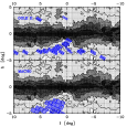
Figure 3: Locations of the fields observed towards the Galactic bulge by the OGLE II (upper panel) and by the MACHO (lower panel) microlensing experiments.

I can now apply the SFD map and the scaling factor obtained in the previous Section to investigate the reddening close to the Galactic plane. In Figure 2 I plot the $E(B-V)$ reddening map of $20\times 10\;\deg$ part of the the Galactic center. Contours correspond to re-scaled $E(B-V)=0.4,0.8,1.5,3.0,5.0,10.0\;$mag. As discussed above, the comparison range of the $E(B-V)_{GC}$ extends only to 1.75, so the derived scaling of $\sim 1.35$ might not apply in high reddening regions very close to the Galactic plane ($|b|<2\deg$). Also, the SFD map gives by its construction the total dust reddening along given line of sight, which for regions close to the Galactic plane might have significant contribution from dust distributed beyond the observed source.

The spatial structure of reddening seen in Figure 2 is very rich, both on large and small scales. Some of the features, such as more dust extinction above the Galactic plane than below the plane, are well known and can be observed even with a naked eye. There is a pronounced “pinch” in the reddening at the $l\sim 0$ longitude, where some of the iso-reddening contours are $1-3\deg$ closer to the Galactic plane than elsewhere in the map. In a low-reddening window near $(l,b)=(0,-2)$ the rescaled reddening is as low as $E(B-V)\sim 0.6\;$mag. Also worth noticing is low-reddening region near $(l,b)=(4,3)$ with the rescaled reddening as low as $E(B-V)\sim 0.55\;$mag.

It is interesting to compare the locations of the fields observed towards the Galactic bulge by the OGLE II (Figure 3, upper panel) and by the MACHO (Figure 3, lower panel) microlensing experiments (Udalski, Kubiak & Szymański 1997; Alcock et al. 1997). Both experiments cover similar areas on the sky ($\sim 12\deg^{2}$) and show significant overlap with each other, with OGLE II taking somewhat better advantage of low-extinction regions close to the Galactic center (such as the window near $(l,b)=(0,-2)$ discussed above). However, OGLE II fields are much better distributed for applications of their data for the Galactic structure studies, such as investigating the properties of the Galactic bar with the red clump giants (Stanek et al. 1997).

We might attempt to define an “optimal” selection of fields to be used for the microlensing studies. This selection naturally depends on the scientific goal of a given study. To maximize the observed microlensing optical depth during the lifetime of the experiment, I define “reddening-adjusted optical depth” as

$$\tau_{E(B-V)}\equiv\tau\exp{[-\kappa E(B-V)]},$$ (1)

where $\tau$ is the standard optical depth for microlensing and the factor $\exp{[-\kappa E(B-V)]}$ is used to reduce $\tau$ in regions of high reddening (and hence extinction). The coefficient $\kappa$ in the exponent can be adjusted to reflect, for example, a photometric band used for observations. To give an example, the microlensing optical depth is highest towards the Galactic center, yet because of the high dust extinction there it is not a good place to monitor microlensing. In Figure 4 I plot $\tau_{E(B-V)}$, using the rescaled SFD map as the source of reddening $E(B-V)$ and the optical depth from the bar model E2 of Stanek et al. (1997, their Figure 12) as the source of $\tau$ (the contribution from the Galactic disk to the microlensing was not included). I took $\kappa=1.0$ for simplicity.

Figure 4: Map of the “reddening-adjusted optical depth” $\tau_{E(B-V)}$ (Equation 1). Contours are plotted at 10, 30, 50, 70 and 90% of the peak value of $\tau_{E(B-V)}$.

In practice, as current microlensing experiments operate in crowding-limited mode, the reddening-adjusted optical depth defined above is not optimal from their point of view. However, with the progressing development of image-subtraction techniques (see recent papers by Alard & Lupton 1998 and Tomaney 1998) one will be able to detect the microlensing events regardless of crowding.

To summarize, the SFD map overestimates the reddening in $|b|<5\deg$ regions by a factor of $\sim 1.35$, but it is a very valuable tool in investigating features in the reddening near the Galactic plane. I limited myself to investigating the central part of our Galaxy, but the SFD map should be also useful for similar studies in other parts of the Galactic plane.

References

- (1)
- (2) Alard, C., & Lupton, R. H., 1998, ApJ, submitted (astro-ph/9712287)
- (3)
- (4) Alcock, C., et al., 1997, ApJ, 479, 119
- (5)
- (6) Alcock, C., et al., 1998, ApJ, 494, 396
- (7)
- (8) Burstein, D., & Hailes, C., 1982, AJ, 87, 1165 [BH]
- (9)
- (10) Gould, A., Popowski, P., & Terndrup, D. M., 1998, ApJ, 492, 778
- (11)
- (12) Harris, W. E., 1996, AJ, 112, 1487
- (13)
- (14) Reed, B. C., Hesser, J. E., & Shawl, S. J., 1988, PASP, 100, 545
- (15)
- (16) Schlegel, D. J., Finkbeiner, D. P., & Davis, M., 1998, ApJ, in press (astro-ph/9710327) [SFD]
- (17)
- (18) Stanek, K. Z., 1996, ApJ, 460, L37
- (19)
- (20) Stanek, K. Z., et al., 1997, ApJ, 477, 163
- (21)
- (22) Stanek, K. Z., 1998, ApJ, submitted (astro-ph/9802093)
- (23)
- (24) Szymański, M., & Udalski, A., 1993, AcA, 43, 91
- (25)
- (26) Tomaney, A. B., 1998, ApJ, submitted (astro-ph/9801233)
- (27)
- (28) Udalski, A., Szymański, M., Kałużny, J., Kubiak, M., & Mateo, M., 1993, AcA, 43, 69
- (29)
- (30) Udalski, A., Kubiak, M., & Szymański, M., 1997, AcA, 47, 319
- (31)
- (32) Webbink, R. F., 1985, in “Dynamics of Star Clusters”, IAU Symposium 113, eds. J. Goodman and P. Hut (Dordrecht: Reidel), 541
- (33)
- (34) Woźniak, P. R., & Stanek, K. Z., 1996, ApJ, 464, 233
- (35)
- (36) Zinn, R., 1985, ApJ, 293, 424
- (37)