The Assembly of Matter in Galaxy Clusters

Abstract

We study the merging history of dark matter haloes that end up in rich clusters, using $N$-body simulations of a scale-free universe. We compare the predictions of the extended Press & Schechter (P&S ) formalism (Bond et al. 1991; Bower 1991; Lacey & Cole 1993) with several conditional statistics of the proto-cluster matter: the mass distribution and relative abundance of progenitor haloes at different redshifts, the infall rate of progenitors within the proto-cluster, the formation redshift of the most massive cluster progenitor, and the accretion rates of other haloes onto it. The high quality of our simulations allows an unprecedented resolution in the mass range of the studied distributions. We also present the global mass function for the same cosmological model. We find that the P&S formalism and its extensions cannot simultaneously describe the global evolution of clustering and its evolution in a proto-cluster environment. The best-fit P&S model for the global mass function is a poor fit to the statistics of cluster progenitors. This discrepancy is in the sense of underpredicting the number of high-mass progenitors at high redshift. Although the P&S formalism can provide a good qualitative description of the global evolution of hierarchical clustering, particular attention is needed when applying the theory to the mass distribution of progenitor objects at high redshift.

1 Introduction

The Press-Schechter formalism (Press & Schechter 1974, hereafter P&S ) and its extensions (Bond et al., 1991; Bower 1991; Lacey & Cole 1993, hereafter LC93) provide a nice framework of analytical predictions for the formation of dark matter haloes in cosmological models of hierarchical clustering. Until now, these predictions have given us the best handle we possess to understand the formation of structure in the real universe, from sub-galactic scales up to the scale of galaxy clusters. It is therefore of great importance to know how reliable this model is, and how it fares when compared to numerical simulations of structure formation.

Although the P&S predictions have been extensively tested against $N$-body results (e.g. Efstathiou et al. 1988; Lacey & Cole 1994, hereafter LC94; Gelb & Bertschinger 1994), numerical techniques are only now reaching a resolution sufficient to extend this comparison to a large range of masses. Due also to this limitation, most studies have been confined to the global mass function, while the predicted properties of halo progenitors have been compared to numerical results only by LC94.

A good understanding of the model and reliability for these conditional statistics is needed in order to reliably predict several observables, like the abundance of progenitors of any class of astrophysical objects, their formation times, their merging rates, and many other properties. These distributions are particularly important for semi-analytical models of galaxy formation (Kauffmann, White & Guiderdoni 1993; Cole et al. 1994), where the extended P&S formalism is used to produce Monte Carlo realizations of the merging histories of dark matter haloes, and these in turn are the starting ingredient for producing galaxy populations in different cosmological models. The evolution of the properties of these populations changes substantially for different choices of parameters in the P&S model.

In this paper we make a detailed analysis of the P&S predictions for the formation of rich galaxy clusters, and compare these to the properties measured in $N$-body simulations of a scale-free Einstein-de Sitter universe. The high mass and force resolution of our simulations is ideal to resolve dark matter haloes over a large mass range. Our result confirms that the P&S theory can be tuned to give a good overall fit of the global mass function. However, we will prove that the P&S model best fitting the global mass function of our simulations is not a good fit to the statistics involving the progenitors of clusters found in the same simulations. This result points to a structural failure of the theory, as the model parameter – namely the collapse threshold $\delta_{c}$, defined below in Section 3.1 – is fixed by the match with the global mass function and cannot be changed when turning to the conditional statistics.

In Section 2 we briefly present the $N$-body simulations used in our study, and describe the method used to define their population of dark matter haloes. In Section 3 we calibrate the P&S model by fitting the global mass function of a set of cosmological simulations. We show that the standard value for the collapse threshold $\delta_{c}=1.69$ provides a good fit to the simulations. In Sections 4 and 5 we consider a sample of clusters extracted from the simulations presented in Section 3: we present several conditional statistics of the cluster progenitors, and compare them with the predictions of the extended P&S formalism. We show that the P&S model, calibrated as in Section 3, is not a good description of the evolution of cluster progenitors. Finally, in Section 6 we discuss our results and summarize the main conclusions of the paper.

2 Method

2.1 The Simulations

The cluster $N$-body simulations studied in this paper have been presented in Tormen, Bouchet & White (1997), where complete details may be found. In summary, our sample consists of nine dark matter haloes of rich galaxy clusters. These have been produced by tailor-made, high-resolution $N$-body simulations, using the initial condition resampling technique described in Tormen et al. (1997). The clusters correspond to the nine most massive objects found in a parent cosmological simulation (White 1994) of an Einstein–de Sitter universe, with scale-free power spectrum of fluctuations $P(k)\propto k^{n}$, and a spectral index $n=-1$, the appropriate value to mimic a standard cold dark matter spectrum on scales relevant to cluster formation. All simulations have a Hubble parameter $H_{0}=50$ km s^-1 Mpc^-1, and are normalized to match the observed local abundance of galaxy clusters (White et al. 1993).

The parent simulation was evolved using a Particle-Particle-Particle-Mesh code (Efstathiou et al. 1985) with $100^{3}$ particles in a $256^{3}$ grid with periodic boundary conditions. The box size is 150 Mpc on a side. The cluster simulations were evolved using a binary tree-code, in proper coordinates, on a sphere of diameter 150 Mpc, with vacuum boundary conditions. The average cluster mass over our high-resolution sample is $M_{v}\simeq 1.1\times 10^{15}M_{\sun}$. Each cluster is resolved by $\approx 20000$ dark matter particles with an effective force resolution of $\sim 25$ kpc which is constant in proper coordinates.

2.2 Identification of dark matter lumps

We used the potential energy of particles to identify the centres of dark matter lumps (Efstathiou et al. 1988). We defined lumps by an overdensity criterion, and included all particles within a sphere of mean overdensity $\delta_{v}=178$, centred on the particle with lowest potential energy. The value $\delta_{v}$ corresponds to the virial overdensity in the model of a spherical top-hat collapse in an Einstein-de Sitter universe. We will call the corresponding radius the virial radius $r_{v}$ of the lump.

Figure 1: The figure shows the progenitor haloes of a cluster in our sample, seen at redshift $z=2.8$; the cluster virial mass at redshift $z=0$ is $M_{v}=7\times 10^{14}M_{\sun}$. The circles show the lumps of matter found by our algorithm, based on local minima of gravitational potential. The radius of each circle is the virial radius of the lump. Lumps contain at least 8 particles. Overlapping circles are only due to projection effects. The most massive cluster progenitor is situated at position (0,0), and is formed by $\approx 1300$ particles. Only particles actually ending up in the final cluster are plotted. Therefore, progenitor haloes which carry only a small fraction of their mass into the final cluster have only few particles drawn within the corresponding circles.

Following Tormen (1997) we limit our analysis to haloes with $n_{v}\geq 8$ particles. We will generally call field particles all particles unclustered or in lumps with $n_{v}<8$. Fig. 1 shows an example of the lumps found by this algorithm. The plot refers to a cluster in our sample, observed at redshift $z=2.8$. Only particles which are progenitors of the final cluster are plotted.

3 Calibration of the P&S model

In this Section we calibrate the P&S model by fitting the predicted global mass function of dark matter haloes to the results of our cosmological simulations. We take the collapse threshold $\delta_{c}$ as a free parameter and determine the value best-fitting the numerical data. We assume a top-hat filtering to define the mass variance $\sigma^{2}(R)$. In this Section, and only here, we use two methods to define the haloes. A standard percolation scheme – the friend-of-friends algorithm (hereafter FOF) – as defined in Davis et al. (1985), and a spherical overdensity criterion (herafter SO), as defined in the previous Section. We do this to demonstrate the robustness of our best fitting results. Having proven that, in the remainder of the paper we will only consider SO haloes.

For the FOF we take a linking length $b=0.2$. With this choice, groups are approximately identified by closed surfaces of local density $\rho/\rho_{b}\approx 1/b^{3}=125$ (factors of 2 or 1/2 may apply, see Frenk et al. 1988; LC94). Following the notation of LC94, we will call ’FOF(0.2) haloes’ the groups of particles found by this algorithm. For the SO haloes we take the virial overdensity $\delta_{v}=178$, and will call them ’SO(178) haloes’. As discussed in LC94, the algorithms we use to define the dark matter haloes are essentially equivalent to those used by LC94.

3.1 Global Mass function

The study of the global mass function requires a full cosmological simulation. Taking advantage of the self-similarity of our model, we present results averaged over ten output times, taken from two different simulations: one is the parent of the cluster simulations presented above, the other is identical to the first in the numerical parameters, and only differs in the realization of the initial conditions. An extensive comparison between the predictions of the P&S formalism and the results of scale-free $N$-body simulations has been performed by LC94. At the end of this Section we will compare our results to theirs.

For an Einstein-de Sitter universe with scale-free power spectrum $P(k)\propto k^{n}$, the fraction of mass in haloes with mass $M$ at redshift $z$, per interval $d\ln M$, is predicted by the P&S formalism to be

$${df_{M}\over d\ln M}(M,z) = {\alpha\over 2}\left({2\over\pi}\right)^{1/2}\left(M\over M_{*}\right)^{\alpha/2}$$ (1)

$$\times \exp\left[-{1\over 2}\left({M\over M_{*}}\right)^{\alpha}\right],$$

where $\alpha=(n+3)/3$. The time dependence enters only through the characteristic non-linear mass $M_{*}(z)=(4\pi/3)R_{*}^{3}\rho_{b}(z)$, with $\rho_{b}(z)$ the background density of the universe at redshift $z$, and $R_{*}(z)$ the scale corresponding to a linear overdensity $\delta_{c}$ of order unity. The specific value of $\delta_{c}$, called collapse threshold, depends on the criterion used to identify dark matter haloes; a sensible starting value is $\delta_{c}=1.69$, the linear extrapolation at collapse for a spherical top-hat. We use a top-hat filter to calculate $M_{*}$. The value of $M_{*}$ for $\delta_{c}=1.69$ is $M_{*}|_{z=0}=6.16\times 10^{13}M_{\sun}$.

The goal of this Section is to determine the value of $\delta_{c}$ (that is, of $M_{*}$) for which Eq. (1) best fits the mass function of haloes from simulations.

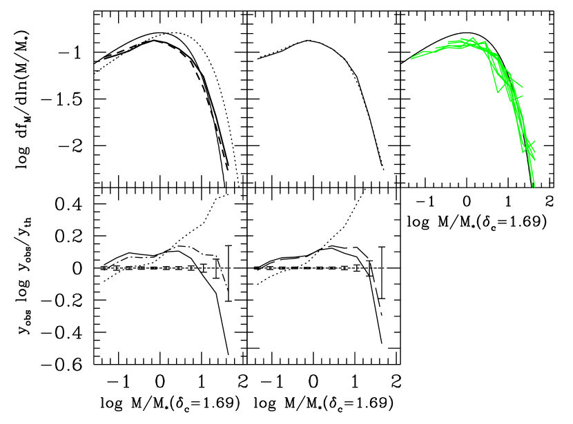
Figure 2: Global mass function for the scale-free cosmological model with $n=-1$. Top Left: Thick curves indicate the values found in simulations, for different group finding algorithm: FOF(0.2) (solid) and SO(178) (short dash). Smooth curves show the values predicted by Eq. (1) for different values of $\delta_{c}$ Top center: The SO(178) curve is shifted by 0.065 along the horizontal axis, showing that its shape is almost identical to the FOF(0.2) curve. Top right: Mass function for 10 different output times (broken curves), taken from two different $N$-body runs of the same model. All outputs agree with the P&S prediction with $\delta_{c}=1.69$ (smooth curve), and there is no systematic variations between the two runs or between different time outputs. This result is shown for FOF(0.2) groups, but identical results are obtained for SO(178) groups. Bottom Left: Logarithmic residuals from the top left panel. for FOF(0.2) groups. Error bars represent the Poissonian $1\sigma$ of the mean around the observed value. Bottom Right: Corresponding residuals for SO(178) groups. Different line types in all panels correspond to different values of $\delta_{c}$: 1.3 (dotted), 1.55 (dot-dash), 1.63 (long dash) and 1.69 (solid).

Fig. 2 presents the global mass function $df_{M}/d\ln M$ for the scale-free model with $n=-1$. The average over different output times was done as described in LC94, weighting the contribution of each curve in each bin by the number of haloes in that bin. To facilitate comparison with LC94, we only used haloes with at least 20 particles.

The top left panel shows the logarithm of $df_{M}/d\ln M$ for FOF(0.2) groups (thick solid), and for SO(178) groups (thick dashed), together with the prediction of Eq. (1) for different values of collapse threshold: the canonical value $\delta_{c}=1.69$ (thin solid) and $\delta_{c}=1.3$ (thin dotted). The choice of the latter value is explained below.

From the figure we see that the mass function from simulations is globally flatter than the P&S prediction, especially at the high mass end. This finding is however in general agreement with previous studies (e.g. Efstathiou et al. 1988, LC94). Despite the slight difference of shape, the $N$-body results are reasonably fitted by the P&S prediction with the canonical choice $\delta_{c}=1.69$, both for FOF(0.2) and SO(178) groups. In fact, the agreement between model and simulation curve in the mass range $-1.4\la\log_{10}(M/M_{*})\la 1.4$ is better than $\approx 40$ percent for FOF(0.2) haloes and better than $\approx 35$ percent for SO(178) haloes. As the shape of the curves from $N$-body is slightly different from the predicted one, best fitting is a rather subjective exercise. However, with the choice $\delta_{c}=1.55$ for FOF(0.2) haloes one can slightly improve the fit at high masses, up to $\log_{10}(M/M_{*})\simeq 1.7$.

The figure also shows that FOF(0.2) groups are slightly more massive than SO(178) groups. In fact, if we shift the SO(178) curve horizontally by 0.065 in $\log_{10}(M/M_{*})$, as in the top central panel, the two curves match almost exactly. Using this scaling between masses of haloes defined by the two algorithms, the best fitting value $\delta_{c}=1.55$ for FOF(0.2) haloes correspond to $\delta_{c}=1.63$ for SO(178) haloes respectively. The residuals between model and $N$-body data, for the considered values of $\delta_{c}$, are plotted in the lower panels of Fig. 2.

The top right panel shows the 10 individual curves used to define the average mass function shown in the top left panel. Note that all outputs agree with the P&S prediction with $\delta_{c}=1.69$ and there is no systematic variations between the two runs or between different time outputs.

3.2 Discussion

Let us compare in more detail our results with those of LC94. These are based on scale-free simulations, one for each spectral index of fluctuations $n=-2$, $n=-1$, $n=0$. LC94 found that the value of $\delta_{c}$ best fitting the mass function of their simulations is $\delta_{c}=1.96$ for the SO(178) haloes and $\delta_{c}=1.81$ for the FOF(0.2) ones. With this choice, they could fit the $N$-body results to better than 30 per cent over a mass range that, for the $n=-1$ simulation, corresponds to $-1.5\la\log_{10}M/M_{*}\la 1.4$. They also found that the canonical value $\delta_{c}=1.69$ still provides a reasonable fit, with an accuracy better than a factor of two on the same mass range for the FOF(0.2) groups.

Our results are generally in good agreement with LC94, as we also find that (a) SO(178) haloes are slightly smaller than FOF(0.2) haloes, and (b) $\delta_{c}=1.69$ is an overall good fit to the data for groups in both identification schemes. Some minor differences are due to the fact that our results are only based on the $n=-1$ model, as opposed to the three scale-free models used by LC94.

Therefore, our robust conclusion is that the P&S model with $\delta_{c}=1.69$ is an appropriate description of the clustering of matter in a global cosmological environment, for both SO(178) and FOF(0.2) dark matter haloes. In the remainder of the paper we will compare the predictions of this calibrated model to the conditional statistics of the progenitors of the most massive clusters found in one of the two simulations presented above.

Another result is that the choice $\delta_{c}=1.3$ gives clearly a bad fit to the global mass function (long dashed lines in Fig. 2), as it predicts far too many high mass haloes. This result is important, as we will show below that, incidently, $\delta_{c}=1.3$ would be the value appropriate to describe the conditional statistics related to the cluster progenitors.

Finally, let us comment on the relative mass of FOF(0.2) and SO(178) haloes. As we mentioned before, haloes identified with a FOF criterion are approximately bounded by a surface of local overdensity $\rho/\rho_{b}\approx 125$ for $b=0.2$. On the other hand, SO(178) haloes are cut at a mean overdensity $<\rho>/\rho_{b}=178$. Since we know the shape of the density profiles for these haloes (Navarro, Frenk & White 1996; Cole & Lacey 1996; Tormen et al. 1997), we can relate these two values. The virial mean overdensity corresponds to a local overdensity $\rho/\rho_{b}\approx 10-30$, weakly depending on the halo mass in terms of $M_{*}$ and on the cosmological model. On the other hand, a local overdensity $\rho/\rho_{b}\approx 125$ corresponds to a mean overdensity $<\rho>/\rho_{b}=500$ (as found also by Frenk et al. 1988), and to a mass $M_{FOF(0.2)}\approx 0.75M_{SO(178)}$, with $M_{SO(178)}$ the virial mass. From this information, we should expect the FOF(0.2) groups to be less massive, not more massive than the SO(178) haloes. Instead we have shown above that, on average, $M_{FOF(0.2)}\approx 1.15M_{SO(178)}$, or about 50 per cent more massive than their expected mass. This difference is probably due to the tendency of FOF to connect structures along bridges and filaments, and is a quantitative evidence that FOF groups are, on average, very aspherical objects.

4 Evolution of cluster progenitors

We now turn our analysis to the cluster simulations. We remind that the clusters analyzed here have been obtained by resimulating at higher mass and spatial resolutions the nine most massive clusters found in one of the two $N$-body runs presented in Section 3.1. In this Section we study the mass function of the cluster progenitors at different redshifts, the evolution of the comoving density of progenitors, and their global infall rate as haloes merge together to form more massive haloes. In the next Section we will concentrate on the most massive cluster progenitor: we will study its formation redshift and the time evolution of the corresponding infall rate. We will prove that the calibrated P&S model (which has $\delta_{c}=1.69$), underpredicts the clustering of high-mass progenitors at high redshift. As mentioned above, in the remainder of this paper we only consider haloes defined by the spherical overdensity criterion SO(178).

In the hierarchical clustering picture of structure formation, matter clusters on small scales first, and haloes of a given mass are formed by the assembly of pre-existing smaller haloes. Therefore, in this model, once an element of matter becomes part of a halo, it will be forever part of some halo from then on. Also, all the matter forming a halo comes from haloes of some mass. Finally, when a satellite lump is accreted onto a more massive halo, all of the satellite mass is incorporated in the more massive object. In this picture the formation of structure is a very lumpy process. This description is fairly close to what we observe in $N$-body simulations of hierarchical clustering, although the actual collapse of structures is more complicated than its idealized version; in particular, satellites may be tidally stripped prior to merger with a more massive haloes, so that only a fraction of the satellite mass becomes part of the accreting system. Also, during violent merging events, energy is re-distributed among the mass elements, and some matter may temporarily exit the virial radius of the newly formed halo, or in principle even become unbound.

Figure 3: Top panel: fraction of the total mass in progenitors which will actually end up within the virial radius of the final cluster. Bottom panel: radius of the sphere centered on the final cluster and enclosing $90\%$, $95\%$, $99\%$, and $100\%$ of the total mass in progenitors.

Let us call, at any given redshift, progenitors of a cluster all haloes containing at least one particle that by $z=0$ will be part of the cluster, and also all field particles which will end up in the final cluster. We can ask: does all the mass of the progenitors end up in the final system? To answer we calculated the ratio $M_{pro}(z)/M_{v}$ of the total mass in progenitors (both in haloes and in field particles) at redshift $z$, to the final cluster mass. This is shown in the upper panel of Fig. 3. Initially, before the formation of any halo, this value is unity. Then, as matter starts to collapse into haloes, progenitor and non-progenitor particles are captured in the same haloes, and $M_{pro}(z)/M_{v}$ increases up to $\simeq 1.2$ at $z\sim 1$. It then remains at his level until $z\simeq 0.2$, then it decreases to reach unity at the final time.

What is the fate of the non-progenitor particles captured in progenitor haloes? That is, where can we find, at $z=0$, the extra $\approx 20\%$ of matter in progenitors shown in the upper panel of Fig. 3? The answer is shown in the lower panel, where we plot the radius of spheres centered on the final cluster and containing different percentages of the total progenitor mass, as identified at different redshifts. For example, we see that 99 per cent of the progenitor particles is situated, at $z=0$, within roughly 2.5 virial radii, and that 100 per cent of them is within 4.5 virial radii. This means that, during the cluster collapse, no particle from the progenitor haloes has actually escaped to infinity. Correspondingly, but implicitly required by the re-simulation technique used for the cluster simulations, no particle from infinity has become part of the final halo. By number, roughly $80\%$ of the progenitor lumps carry at least $80\%$ of their mass into the final cluster, while only $10\%$ carry less than $20\%$ of their mass, in fair agreement with the theoretical picture.

A final remark is on resolution issues. The gravitational softening of our simulations is constant in proper coordinates. Since at high redshift haloes of a given mass are smaller, they are also more poorly resolved. As a softening comparable to the halo size introduces a bias in the halo mass, in this section we conservatively consider only progenitor haloes with virial radius larger than $100$ kpc, or four times the gravitational softening. This will result in a time dependent low mass cutoff in the statistics we are going to present.

4.1 Conditional mass function

In this section we fit the calibrated P&S model to the conditional mass function of cluster progenitors. In the P&S formalism, the mass fraction in progenitor haloes of a given mass can be easily calculated. Eq.(2.15) of LC93 gives the differential mass distribution $df_{M}(M,z|M_{2},z_{2})/d\ln M$ of haloes at redshift $z$, conditioned by the requirement that the matter will be in a cluster of given mass $M_{2}$ at redshift $z_{2}<z$. For cosmological models with scale-free power spectrum of fluctuations: $P(k)\propto k^{n}$, the equation reads

$${df_{M}\over d\ln M}(M,z|M_{2},z_{2}) = \alpha(2\pi)^{-1/2}\left(M\over M_{*}\right)^{\alpha/2}{(z-z_{2})\over(1-x^{\alpha})^{3/2}}$$ (2)

$$\times \exp\left[{-(z-z_{2})^{2}\over 2(1-x^{\alpha})}\left({M\over M_{*}}\right)^{\alpha}\right]$$

where $x=M/M_{2}$. In our case we take $z_{2}=0$ as the present time in Eq.(2), and $M_{2}=M_{v}$ as the final cluster mass. The fraction of mass in haloes with mass larger than $m_{v}$ at redshift $z$ is easily obtained by integrating Eq.(2) over M, from $m_{v}$ to infinity. The resulting cumulative mass function is

$$f_{M}(M>m_{v},z|M_{v}) = {\mathrm{e}rfc}\Bigl{\{}{z\over\sqrt{2}}\left({m_{v}\over M_{*}}\right)^{\alpha/2}$$ (3)

$$\times \left[1-\left({m_{v}\over M_{v}}\right)^{\alpha}\right]^{-1/2}\Bigr{\}}.$$

In Figs 4 and 5 we compare the differential and cumulative mass function of progenitors Eq.(2) and Eq.(3) to the corresponding statistics from our simulations. Abscissa are normalized to the final mass of the cluster.

Figure 4: Differential mass function progenitors at different redshifts. Each panel shows the mass function of the cluster progenitors, averaged over the cluster sample. Error bars are $1\sigma$ of the distribution, calculated from 100 bootstrap resamples of the actual sample. The smooth solid curve represents the calibrated P&S prediction (Eq.(2) with $\delta_{c}=1.69$). The smooth dotted curve is a P&S model with $\delta_{c}=1.3$.

Figure 5: Cumulative mass function of progenitors at different redshifts. The thick solid curves are the simulation result. The thin smooth curves show the predictions of Eq.(3), with $\delta_{c}=1.69$ (solid line) and $\delta_{c}=1.3$ (dotted line) respectively.

Data from all nine clusters are weighted by the number of particles in progenitors, and combined together. Each panel refers to a different time output, labeled by the average redshift over the sample. For the differential mass function, error bars were obtained from $100$ bootstrap resampling of the data. That is, for each bin they indicate the $1\sigma$ dispersion of the distribution of 100 re-samples of 9 clusters each, each re-sample randomly drawn with replacement from the original collection of 9 clusters. The total number of progenitors in each histogram varies from over 2000 at high redshift to a few hundred close to $z=0$. Histograms are built using the virial mass of the progenitor haloes.

It is clear from the two figures that the calibrated P&S model (Eqq. (2), (3), smooth solid curves) is not a good fit to the numerical data. Specifically, it underestimate the number of massive progenitors by up to one order of magnitude at redshift $z\ga 1$. Now, it happens that the simulation results are reasonably fit by a P&S model with $\delta_{c}=1.3$ (corresponding to $M_{*}|_{z=0}=1.35\times 10^{14}M_{\sun}$, dotted curve). However, the collapse threshold has been fixed by the fit to the global mass function and is not a free parameter anymore. Therefore, the dotted curve must be considered only as a rough quantitative measure of the discrepancy between the calibrated P&S model (which has $\delta_{c}=1.69$) and the simulations.

In the present analysis we have used the total mass of the progenitor haloes. However we found that the result does not change if instead one uses, for each progenitor, the actual fraction of halo mass ending in the final cluster.

4.2 Comoving density of progenitors

Another way to look at the same results is to consider the comoving density $\rho_{pro}(z)$ of progenitor haloes in a given mass range $[M_{a},M_{b}]$, at different redshifts. This is easily obtained as an integral over Eq. (2):

$$\rho_{pro}(M_{a},M_{b},z|M_{2},z_{2}) = \rho_{b}\int_{\ln M_{a}}^{\ln M_{b}}$$ (4)

$${df_{M}\over d\ln M}(M,z|M_{2},z_{2}){d\ln M\over M}.$$

The corresponding number of progenitors per cluster in the same mass range is $N_{pro}(z)=\rho_{pro}(z)M_{2}/\rho_{b}$. This quantity is similar to the comoving density of haloes usually calculated from the global mass function Eq. (1), which is often compared to the observed abundance of some class of extragalactic objects; it differs however in the interpretation. The comoving density Eq. (4) in fact refers to proto-cluster matter, and so it only applies to regions of the universe initially overdense, and unusually populated. This conditional density can therefore be used to estimate the predicted comoving density of objects which populate the environment of a proto-cluster.

In Fig. 6 we show comoving density for four different mass ranges and for $z_{2}=0$. In each panel, the number of progenitors per comoving cubic Mpc is plotted versus redshift: the symbols show the average value over the cluster sample. Virial masses for the progenitor SO(178) haloes are considered.

Figure 6: Comoving density of progenitor haloes in different mass ranges, compared with the extended P&S prediction, versus redshift. The solid squares show the average number of haloes per comoving cubic Mpc, measured in the simulations. The smooth solid curve is the conditional calibrated P&S prediction Eq. (4). The dashed line is the corresponding prediction for an unconstrained environment, obtained by inserting Eq. (1) in Eq. (4). The dotted curve is a conditional P&S prediction with $\delta_{c}=1.3$.

The solid curve is the conditional density predicted by the calibrated P&S model. For comparison, the dashed line shows the corresponding global comoving density obtained by inserting the global mass distribution Eq.(1) into Eq. (4). The P&S model is for a final halo of mass $M_{v}=1.1\times 10^{15}M_{\sun}$, the average cluster mass for our sample. Again we see that the calibrated P&S model (solid curve) underestimates the clustering of high-mass progenitor by up to two orders of magnitude at high redshift. Again, the discrepancy is roughly described by a change in collapse threshold ($\delta_{c}=1.3$, dotted curve).

4.3 Global infall rates

A measure of the rate at which the proto-cluster matter merges into more and more massive haloes is given by the time derivative, at any fixed mass, of the cumulative mass function Eq.(3). The expression is (Bower 1991)

$${\partial f(m_{v},z|M_{v})\over\partial t} = {\partial\over\partial x}{\mathrm{e}rfc}(x_{M}){\partial x\over\partial z}{\partial z\over\partial t}$$ (5)

$$= \left({2\over\pi}\right)^{1/2}{2\over 3}(1+z)^{5/2}\left({m_{v}\over M_{*}}\right)^{\alpha/2}$$

$$\times \left[1-\left({m_{v}\over M_{v}}\right)^{\alpha}\right]^{-1/2}$$

$$\times \exp\Bigl{\{}{z^{2}\over 2}\left({m_{v}\over M_{*}}\right)^{\alpha}\left[1-\left({m_{v}\over M_{v}}\right)^{\alpha}\right]^{-1}\Bigr{\}},$$

with $x_{M}$ the content of the curled brackets in Eq. (3). More specifically, Eq. (5) gives the global rate at which progenitors with mass smaller than $m_{v}$ merge together and form progenitors of mass larger than $m_{v}$, at redshift $z$. This quantity has been called infall rate by Bower (1991). Therefore, we keep this definition, although we will distinguish below between the global infall rate of progenitors, given by Eq. (5), and the infall rate of haloes onto the main cluster progenitor, which we calculate in Section 5.2. It is in fact important to remember that Eq. (5) does not contain any information on the relative mass of the merging haloes, nor does it distinguish mergers onto the most massive cluster progenitor from other encounters between progenitors.

Figure 7: The figure shows the global infall rates of cluster progenitors, as a function of redshift, for different threshold mass $m_{v}/M_{v}$.

It is useful to plot the information of Eq. (5) as a function of the lookback time from $z=0$. This is done in Fig. 7, where we compare the predictions of Eq. (5) with the infall rate measured from the simulations, taking the numerical derivative of the curves shown in Fig. 5. Rate units are fraction of the final cluster mass per Gyr.

Each panel shows the infall rate for a given mass threshold, in terms of the final cluster mass. The calibrated P&S prediction (solid curve) is systematically shifted to lower lookback times for $m_{v}/M_{v}>0.01$, compared to the numerical results. The dotted curve is a P&S model with $\delta_{c}=1.3$, shown to quantify this discrepancy.

5 Formation of the main progenitor

In the previous Section we have considered the global evolution of all progenitors of a present-day cluster. A different way to estimate the speed at which the cluster grew is to look at the formation of the most massive cluster progenitor, which we do in the present Section. We will focus on the redshift at which the main progenitor formed, and on the infall rate of other cluster progenitors onto it.

Operationally, we define the main (or largest) progenitor of a cluster, at any given redshift, as the progenitor halo containing the largest fraction of the mass from the final cluster. In all cases this coincided with the most massive progenitor, although, with the present definition, the main cluster progenitor in $N$-body simulations is not necessarily the most massive one, as progenitors carry different fraction of their mass into the final cluster.

5.1 Formation redshift

The cluster formation redshift is usually defined as the earliest redshift at which the largest cluster progenitor reached at least $50\%$ of the cluster’s final mass. The argument given by LC93 to estimate formation redshifts is the following. The probability for a cluster of present mass $M_{2}$ to have had at least a progenitor of mass $M$ at redshift $z$ is simply the probability in Eq. (2) times the average number $M_{2}/M$ of progenitors with mass $M$. Since each object can have at most one progenitor with half or more of its proper mass, the probability that a cluster had a progenitor with mass $xM_{2}$, with $0.5<x<1$, at redshift $z$, is the integral quantity

$$p(M>xM_{2},z|M_{2},z_{2})=\int_{\ln(xM_{2})}^{\ln M_{2}}d\ln M\left({M_{2}\over M}\right){df\over d\ln M}$$ (6)

with $z_{2}=0$, and $df/d\ln M$ given by Eq. (2). For $x=0.5$ LC94 found a good agreement between this prediction and their $N$-body simulations, for different cosmological models with scale-free power spectrum. Here we compare our data with the same prediction, allowing however different values of $x$ between $0.5$ and $1$, to consider a larger part of the cluster formation history.

Fig. 8 shows the probability distribution function in redshift for the mass of the main cluster progenitor. Symbols indicate the actual formation history of the largest progenitor, normalized to the final cluster mass, and averaged over the cluster sample. Error bars give the $1\sigma$ dispersion of the sample distribution. For each value of $x=M(z)/M_{2}(z=0)$, redshifts are indicated which correspond to the mean (thick solid line), and to the 5, 25, 50, 75 and 95 percentiles (dotted, dashed and thin solid lines) of the distribution obtained using Eq. (6). The upper panel compares the data to the calibrated P&S model; and the lower panel to the P&S model with $\delta_{c}=1.3$. The predictions are for a cluster with mass equal to the mean mass of the sample, $M_{v}=1.1\times 10^{15}M_{\sun}$. Symbols above the mean indicate early formation, and viceversa.

Figure 8: Cluster formation redshift. Solid squares show the time growth of the largest cluster progenitor, averaged over the sample, and normalized to the final cluster mass. Error bars indicate $\pm 1\sigma$ of the distribution. The other lines are obtained from Eq. (6), and indicate the 5, 25, 50, 75 and 95 percentiles (dotted, dashed and thin solid) and the mean (thick solid) of the predicted formation redhift for a cluster with mass $M_{v}=1.1\times 10^{15}M_{\sun}$, the sample mean mass. Panel (a) compares the data to the predictions for the calibrated P&S model ($\delta_{c}=1.69$). Panel (b) is for $\delta_{c}=1.3$.

The figure confirms the picture above: the sample clusters form earlier than predicted by the calibrated P&S model. For seven out of nine objects, the mass of the largest progenitor is always above the mean predicted at each redshift, while three clusters actually have a history at, or outside, the 95% percentile of the predicted distribution. For comparison, Fig. 8b shows a P&S prediction with $\delta_{c}=1.3$, which provides a better description of the numerical data.

5.2 Accretion rates

We now consider the evolution of the halo infall onto the most massive cluster progenitor. For clarity of terms, hereafter we will call the corresponding rate the cluster accretion rate, not to confuse it with the infall rate discussed in the previous Section.

Unlike the global infall rate, which can be calculated analytically, the P&S prediction for the accretion rate onto the main progenitor requires the use of Monte Carlo merging trees, as the extended P&S formalism does not contain, by itself, a rule on how to break up the final cluster in smaller progenitors as one goes back in time. To establish such a rule requires some extra assumptions, and different assumptions lead to different ways to construct merging trees. However, although these may lead to differences in the details of the merging history, they should give similar global results (Kauffman & White 1993).

The expression for the infall rate Eq. (5) does not distinguish between infall onto the most massive cluster progenitor and mergers between other progenitors. On the other hand, it is often useful to have the rate of infall on the main progenitor of the cluster, especially if one wishes to compare the latter to some observation. A classical example is the Butcher-Oemler effect (Butcher & Oemler 1978): the fraction of blue, star-forming galaxies in clusters increases rapidly with redshift, so that in clusters at $z\sim 0.4$ it is a factor of $\sim 10$ higher than in clusters observed locally.

Two mechanisms have been advanced to give a physical explanation to the starburst of these galaxies. The first is the infall hypothesis (Dressler & Gunn 1983), where star formation is triggered by ram-pressure from the intracluster medium, during the first infall of an accreted galaxy in the cluster potential. A second idea (Lavery & Henry 1988) is that galaxy-galaxy collisions in the cluster environment are responsible for the starburst.

Clusters formed in a hierarchical scenario have a history which is qualitatively consistent with both mechanisms (Bower 1991; Kauffmann 1995). In fact, a cluster of given physical mass is a much younger object at high than at low redshift. Therefore, both the infall of haloes and the merging of its progenitors are stronger at high redshift. In these models, the quantity used to measure the infall of galaxies onto the cluster has usually been the global infall rate presented in Section 4.3 (Bower 1991), or the fraction of cluster mass in galaxy-size haloes (Kauffmann 1995). However, the accretion rate onto the main cluster progenitor is probably a more appropriate quantity to consider. This differs from the global infall rate especially early in the cluster formation history (high lookback times), when most of the infall is between progenitors other than the most massive one.

To highlight the difference between the accretion history of clusters observed at $z=0$ and at higher redshift, we divided our sample of nine objects in two subsets: a first one containing the five less massive clusters, which we will observe at $z=0$ and will call low redshift (L) sample; and a second one with the four more massive clusters, which we will observe at $z\sim 0.55$ and will name high redshift (H) sample. As the average cluster mass in these two subsets at the time of observation is roughly the same, $M_{v}\approx 6\times 10^{14}M_{\sun}$, we are looking at clusters of the same physical size at both redshifts, although the (H) clusters are more massive in terms of $M_{*}$.

Figure 9: Accretion rate onto the main cluster progenitor as a function of lookback time. The figure shows the mass fraction accreted in haloes of mass $m_{v}\in[4\times 10^{11},10^{13}]M_{\sun}$ per Gyr by clusters of average final mass $6\times 10^{14}M_{\sun}$. Squares correspond to the low redshift sample (L), circles to the high redshift sample (H). Error bars are $1\sigma$ of the sample mean.

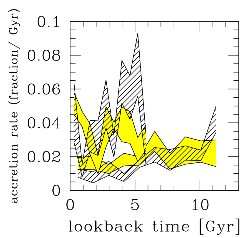
Figure 10: The figure is the analog of Figure 9, but now plotting the prediction of the merger tree based on the extended P&S formalism. The bands enclose $\pm 1\sigma$ (of the mean) around the mean rate.

Fig. 9 shows, for the two subsets, the evolution of the average accretion rate onto the main cluster progenitor, as a function of lookback time. Only accretion of galaxy-size haloes is considered: $m_{v}\in[4\times 10^{11},10^{13}]M_{\sun}$. Squares show the accretion rate for low redshift (L) clusters, circles for (H) clusters. The corresponding global infall rate, for (L) clusters, is in-between that of the two upper panels of Fig. 7. For the reason explained above, the (L) accretion rate is a much flatter function of lookback time than the global infall rate, and is only slightly peaked at very high lookback times. On he contrary, accretion in (H) clusters mostly happens very recently, when it is up to four or five times bigger than the accretion rate for the (L) clusters.

Fig. 10 shows the merging tree predictions to be compared to Fig. 9. The plotted bands enclose $\pm 1\sigma$ of the mean of the accretion rate on two samples of clusters with the same characteristics as the two $N$-body subsets. Solid bands are the prediction of the calibrated P&S model; hatched bands are a P&S model with $\delta_{c}=1.3$. As can be seen, accretion is stronger for the (H) sample, and weaker for the (L) sample, as in the $N$-body case. However, the predictions of different $\delta_{c}$ do not differ appreciably. This is partly consequence of the large scatter in the predicted rates. However, the main reason for the similarity is that here we consider accretion of galaxy-size haloes, and for such haloes the two models predict similar abundances (as shown in Fig. 6) and have similar global infall rates (from Fig. 7). We therefore conclude that the accretion rate on the main cluster is not sensitive to the value of $\delta_{c}$.

Finally, Fig 10 shows large variations in the accretion rates of the (H) sample as a function of lookback time, even within the same model. This result suggests that even high redshift clusters can sometimes exhibit, at the time of observation, a weak accretion rate, and that this is consistent with the discrete nature of matter infall. Such “weakly accreting” clusters could be naturally associated to observations of “non Butcher-Oemler” clusters.

6 Discussion and Conclusions

We have studied the merging history of rich clusters, using $N$-body simulations of an Einstein-de Sitter universe, with scale-free power spectrum of fluctuations, and spectral index $n=-1$. Our results are summarized as follows.

1. The formation process of dark matter haloes in our simulations satisfies the assumptions of the hierarchical clustering model with reasonable accuracy.

2. The global P&S mass function Eq. (2) provides a good fit to $N$-body data. Although $df_{M}(M)/d\ln M$ from simulations is slightly flatter than predicted, the standard choice $\delta_{c}=1.69$ produces a mass function which agrees with the $N$-body data to better than 40 percent in the range $-1.4\la\log_{10}(M/M_{*})\la 1.4$, for both FOF(0.2) and SO(178) haloes. This conclusion agrees with earlier work (e.g. Efstathiou et al. 1988; LC94). A finer tuning in the value of the threshold density: $\delta_{c}=1.55$ for FOF(0.2) haloes and $\delta_{c}=1.63$ for SO(178) haloes slightly extends the agreement at the high mass end of the mass function.

3. In contrast with the previous point, the assembly of matter in a proto-cluster environment takes place earlier than predicted by the P&S model calibrated with $\delta_{c}=1.69$. As a consequence, this choice underestimates the growth of structures especially at the high mass tail and at high redshift. For example, the abundance of galaxy groups at redshift $\approx 5$ is underestimated by almost two orders of magnitude.

   The discrepancy between theory and numerical data can be modeled by a simple variation of the collapse threshold: a value $\delta_{c}=1.3$, which corresponds to a typical nonlinear mass $M_{*}$ more than two times larger than that of the calibrated P&S model, would give a much better fit to the $N$-body data. However, $\delta_{c}$ was fixed at $1.69$ by the requirement that the P&S model best-fits the global mass function, and is not a free parameter anymore.

4. The accretion rate of galaxy-size haloes onto the main cluster progenitor is not sensitive to the choice of $\delta_{c}$, as it samples a mass range where the difference between the two considered models are not significative.

The fact that the P&S model, calibrated to fit the global mas function, is unable to describe the clustering of a constrained environment suggests that the P&S model and extensions, in their present formulation, may be structurally inadequate to give a consistent description of the gravitational clustering of matter in a general context. Such a conclusions would have important theoretical consequences if confirmed by future work.

We stress that the present result has nothing to do with the different values of $\delta_{c}$ found by several authors when fitting the global mass function (e.g. Efstathiou et al. 1988; Gelb & Bertschinger 1994; LC94). As clearly dicussed by LC94, there the discrepancies were mainly due to different choices for the algorithm used to define dark matter haloes and for the filter used to define the linear prediction. On the contrary, we find that the value of $\delta_{c}$ that best-fits the global mass function is inadequate to fit the statistics of halo progenitors which come from the same simulations, and are defined using the same group-finding algorithm and linear filter. Such comparison has never been done before and highlights a novel weakness of the P&S model.

One possibile interpretation of the present results is that the value of the collapse threshold appropriate for the conditional statistics might depend on the mass of the final object relative to the value of $M_{*}$. In this interpretation, $\delta_{c}$ would be regarded as a free parameter to be fixed as a function of mass. The value we found, $\delta_{c}=1.3$, would then be suitable for rich clusters, i.e. objects with $M\ga 10M_{*}$. Higher values might instead be required to fit the conditional statistics of smaller haloes, so that the standard threshold collapse value, $\delta_{c}=1.69$, would result from the average of a continuous set of different values over the entire halo population.

A physical explanation of such a dependence could be the departure from spherical collapse (Bond & Myers 1996; Monaco 1995) in a mass-dependent manner; another could be some systematic difference in the properties of the initial conditions for objects of different mass. To test the first possibility, we measured the infall pattern of matter for the clusters in our sample, using the axial ratios of the ellipsoid defined by satellite infall onto the main cluster progenitor (as in Tormen 1997). We did not find any systematic difference between high and low mass clusters; however our sample is too small in number and in mass range to make a definitive statement on this point. The second possibility requires a more targeted analysis, again using a larger cluster sample and spanning a larger mass range, and work is in progress in this direction.

In the light of the present results, we conclude by stressing that the P&S model should be used with care when describing the clustering properties of halo progenitors, as such description, in its standard formulation, is not accurate.

References

- [] Bond J.R., Myers, S.T., 1996, ApJS, 103, 41
- [] Bond J.R., Cole S., Efstathiou G., Kaiser N., 1991, ApJ, 379, 440
- [] Bower R.G., 1991, MNRAS, 248, 332
- [] Butcher H.R., Oemler A., 1978, ApJ, 219, 18
- [] Cole S., Lacey C.G., 1996, MNRAS, 281, 716
- [] Cole S., Aragòn Salamanca A., Frenk C.S., Navarro J.F., Zepf S.E., 1994, MNRAS, 271, 781
- [Efstathiou et al. 1985] Davis M., Efstathiou G., Frenk C.S., White S.D.M., 1985, ApJ, 292, 371
- [] Dressler A., Gunn J.E., 1983, ApJ, 270, 7
- [Efstathiou et al. 1985] Efstathiou G., Davis M., Frenk C.S., White S.D.M., 1985, ApJS, 57, 241
- [Efstathiou et al. 1988] Efstathiou G., Frenk C.S., White S.D.M., Davis M., 1988, MNRAS, 235, 715
- [Efstathiou et al. 1988] Frenk C.S., White S.D.M., Davis M., Efstathiou G., 1988, ApJ, 327, 507
- [] Gelb J.M., Bertschinger E., 1994, ApJ, 436, 467
- [] Kauffmann G., 1995, MNRAS, 274, 160
- [KW93] Kauffmann G., White S.D.M., 1993, MNRAS, 261, 921
- [KWG93] Kauffmann G., White S.D.M., Guiderdoni B., 1993, MNRAS, 264, 201
- [1993] Lacey C.G., Cole S., 1993, MNRAS, 262, 627 (LC93)
- [1994] Lacey C.G., Cole S., 1994, MNRAS, 271, 676 (LC94)
- [] Lavery R.J., Henry J.P., 1988, ApJ, 330, 596
- [] Monaco P., 1995, ApJ, 447, 23
- [1996] Navarro J.F., Frenk C.S., White S.D.M., 1996, ApJ, 462, 563 (NFW)
- [] Press W.H., Schechter P., 1974, ApJ, 187, 425
- [] Tormen G., 1997, MNRAS, 290, 411
- [] Tormen G., Bouchet F.R., White S.D.M., 1997, MNRAS, 286, 865
- [] White S.D.M., 1994, unpublished
- [] White S.D.M., Navarro J.F., Evrard A.E., Frenk C.S., 1993, Nature, 366, 429