Variance and Skewness in the FIRST Survey

Abstract

We investigate the large-scale clustering of radio sources in the FIRST 1.4-GHz survey by analysing the distribution function (counts in cells). We select a reliable sample from the the FIRST catalogue, paying particular attention to the problem of how to define single radio sources from the multiple components listed. We also consider the incompleteness of the catalogue. We estimate the angular two-point correlation function $w(\theta)$, the variance $\Psi_{2}$, and skewness $\Psi_{3}$ of the distribution for the various sub-samples chosen on different criteria. Both $w(\theta)$ and $\Psi_{2}$ show power-law behaviour with an amplitude corresponding a spatial correlation length of $r_{0}\sim 10h^{-1}$Mpc. We detect significant skewness in the distribution, the first such detection in radio surveys. This skewness is found to be related to the variance through $\Psi_{3}=S_{3}(\Psi_{2})^{\alpha}$, with $\alpha=1.9\pm 0.1$, consistent with the non-linear gravitational growth of perturbations from primordial Gaussian initial conditions. We show that the amplitude of variance and skewness are consistent with realistic models of galaxy clustering.

1 INTRODUCTION

Surveys of optical and infrared galaxies have revealed the rich structure of the universe and have provided much information on the large-scale structure out to redshifts $z\sim 0.1$ (e.g. APM, Maddox et al., 1990 and IRAS, Fisher et al., 1993). In contrast radio sources, although representing only a small fraction of all galaxies, can be detected over significant cosmological distances (up to $z\sim 4$), sampling much larger volumes of space and therefore with the potential to provide information on much larger physical scales.

It had been suggested (Kaiser, 1984) that galaxies form preferentially in high-density peaks of the underlying mass distribution. If it is true, then the statistics of galaxy distributions provide us with information, although biased, about the underlying matter distribution.

It has long been debated whether radio galaxies are clustered or isotropic on the largest scale. The study by Webster (1976), which looked at 8000 radio sources, found $<3\%$ variability in the number of sources in randomly-placed 1-Gpc cubes. This led to a widely-accepted view that radio sources were isotropically distributed. Even if this were not true, the large range in intrinsic luminosity of radio sources might effectively wash out structures when the distribution is projected onto the sky with information about radial distribution effectively lost. Other studies (Seldner & Peebels (1981), Shaver & Pierre (1989)) reported a detection of slight clustering of nearby radio sources, while Benn & Wall (1995) and Baleisis et al. (1998) discussed other measures of anisotropy in radio surveys. Clustering in the 4.85 Ghz Green Bank (87GB: Gregory & Condon, 1991) and in the Parkes-MIT-NRAO (PMN: Griffith & Wright, 1993) catalogues was studied by correlation-function analysis (Kooiman et al., 1995; Sicotte, 1995; Loan, Wall & Lahav, 1997). These studies indicated that radio objects are actually more strongly clustered than local optically-selected galaxies. This conclusion was confirmed by correlation analysis of the FIRST survey (Cress et al., 1996).

One of the possible ways of investigating clustering properties of radio sources is by means of the distribution function (counts in cells) i.e. the probability of finding $N$ galaxies in a cell of particular size and shape. This analysis includes all the moments of the distribution function and therefore provides a more complete description of large-scale structure. Furthermore it can be shown (Peebles, 1980; Frieman & Gaztañaga, 1994) that the higher-order moments of the galaxy distribution can be used as a test of non-linear models for large-scale structure.

This paper presents a counts-in-cells analysis carried out for the FIRST radio survey. We focus on the second and third moment of the distribution together with the angular two-point correlation function of the sample, and we test the predictions of different cosmological models. We report a detection of skewness $S_{3}=\Psi_{3}/\Psi_{2}^{2}=const$ (with $\Psi_{2}$ and $\Psi_{3}$ defined as the second and the third moment of the distribution). Our measurement accords with the hypothesis of non-linear growth of observed structures by gravitational clustering from initially-Gaussian density fluctuations.

In Section 2 we describe the catalogue in its original form and explain the procedures providing us with modified samples analysed in the rest of the paper. In Section 3 we present the results of our analysis for the angular two-point correlation function, and the angular second and third moments of the distribution. Section 4 discusses the deprojection of our 2-d measurements to estimate the quantities describing spatial distribution. Section 5 summarises our conclusions.

2 THE DATA

2.1 The Public Catalogue

The FIRST (Faint Images of the Radio Sky at Twenty centimetres) survey (Becker et al., 1995) began in the spring of 1993 and will eventually cover 10,000 square degrees of the sky in the north Galactic cap. The VLA is being used in B-configuration to take 3-min snapshots of 23.5-arcmin fields arranged on a hexagonal grid. The observations are at 1.4 GHz and the beam-size is 5.4 arcsecs, with an rms sensitivity of typically 0.14 mJy/beam. A map is produced for each field and sources are detected using an elliptical Gaussian fitting procedure (White et al., 1997). The 5-rms source detection limit is roughly 1 mJy. This survey is 50 times more sensitive than any previous large-area radio survey (see White et al., 1997 for details), leading to a high surface density of objects in the catalogue ($\sim 100$ per square degree). It therefore provides an excellent tool for investigating the clustering properties of faint sources.

The catalogue is still in the process of construction, but nevertheless is publically accessible. We used the 27 Feb 1997 version which contains approximately 236,000 entries and is derived from the 1993 through 1996 observations covering about 2575 square degrees, including most of the area $7^{h}20^{m}<{\rm RA}(2000)<17^{h}20^{m}$, $22.2^{\circ}<{\rm Dec}<42.5^{\circ}$. The sky coverage is available in the form of a map of rms sensitivity at 3-arcmin resolution. To simplify our clustering analysis we restricted the area to $7^{h}44^{m}<{\rm RA}<17^{h}20^{m}$, $22.4^{\circ}<{\rm Dec}<41.8^{\circ}$, which has essentially complete coverage.

Within this area there are regions of low source-density because the original catalogue includes only sources brighter than 5 rms. In calculating the counts-in-cells statistics in the following sections we used the coverage map of the survey to ‘mask out’ all those cells in which the noise was large enough to reduce the number of images in the catalogue, ie 0.2 mJy for a flux limit of 1 mJy, and 0.6 mJy for a flux limit of 3 mJy. When we analyse cells significantly larger than the coverage pixels, we reject a cell only if the fraction of useful area is less than 0.75. We keep cells with a ratio $\frac{useful\;area}{total\;area}\;>\;0.75$, and correct the count in each cell by the ratio of useful to total area. For the angular correlation-function analysis we corrected for these effects by generating random catalogues modulated by the rms sensitivity from the coverage map.

The public catalogue is not immediately suitable for clustering analysis, as there are spurious images from sidelobes of bright sources, and single sources are frequently listed as multiple components. These “extra” sources would artificially increase the observed clustering in the catalogue. Probable side-lobes have been identified using an oblique decision-tree program and are flagged in the catalogue (White et al., 1997). We simply rejected all the flagged sources from the original catalogue. We investigate the problem of multi-component sources in some detail in the next section.

We initially chose the flux limit of 1 mJy, corresponding to a 5-rms source detection (as discussed in more detail in Section 2.3). In this way we chose a sample of 189,689 sources from the raw catalogue. We label this sample as C1.

2.2 Multi-component Sources

Radio sources often have widely-separated components corresponding to the nucleus with hot-spots along and at the end of the jets. If the shape of a source is complex, the source detection algorithm fits several components to reproduce the shape. These two effects mean that a single radio source can appear in the catalogue split into two or more sub-components. If analysed as single sources, these components would seriously distort clustering measurements, with effects particularly serious for higher order moments which are more sensitive to tight groupings.

We have investigated techniques to identify tight groups of sources likely to be sub-components of a single radio source. For each group we replace all of the sub-components by a single source with flux equal to the sum of the individual fluxes, placed at the mean position. As described in the following sections, this recombining procedure is of crucial importance in the analysis of the clustering.

Following Cress et al. (1996), using a percolation technique we first simply identified all groups of sources within $0^{.}02^{\circ}$ of each other; each such group was replaced by a single source. This procedure found 25447 groups with a mean of 2.36 sources per group. A histogram of the number of groups as a function of the number of sources in the group is shown in Figure 1. Since the position and flux of the new composite source is different from the individual sub-components, it is possible that the new source can be grouped with other sources. To ensure that all groups were located, we re-ran the group-finding procedure on the revised catalogue repeatedly until no new groups were found. This produced just 10 extra groups, leaving a catalogue of 155,084 sources. We refer to this sample as C2.

Figure 1: Number of component groups derived after the combining procedure vs the number of objects in each group. The solid line shows the results obtained by combining sources according to their separation ($\theta_{link}=0.02^{\circ}$); the dotted line is given by adding a procedure for removing spurious aggregations according to a flux-separation relationship, while the dashed line includes a constraint on the flux ratio.

This procedure efficiently combines sub-components into a single composite source, but can also combine physically-distinct sources into a single source, with drastic effect on the apparent clustering in the catalogue (see Figure 5). We have attempted to improve on this simple approach by varying the link-length in the percolation procedure according to the flux of each source. This is motivated by the well-known $\theta-S$ relation, extended by Oort (1987) to low flux densities, and shown to follow $\theta\propto\sqrt{S}$.

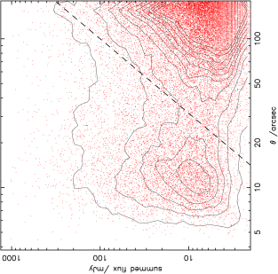
Figure 2: Sum of the fluxes of the components of double sources as a function of their separation. We chose to combine pairs which lie to the left of the dashed line (see text for details).

In order to determine a reasonable flux–separation relation, we plot the sum of the fluxes of the components of each apparent double versus their separation up to $0.05^{\circ}$, as shown in Figure 2. Superimposed on this scatter plot, we show contours of the density of points in the $\theta$–flux plane. There are two distinct regions of high density: one on the lower-right and the other on the lower-left of the figure. We inspected maps from the FIRST survey showing 4.5-arcmin squares around a sample of these objects, and found that the peak on the left consists mostly of sub-components of sources as evidenced by trailing substructures between them. The peak on the right consists of independent pairs of sources.

We set the maximum link-length to be proportional to the square-root of the summed flux, $F_{TOT}$,

$$\theta_{link}=100\left(\frac{F_{TOT}}{100}\right)^{0.5}arcsec.$$ (1)

This line is shown by the dashed line in Figure 2 and roughly follows the minimum source-density between the two peaks. Varying the link-length with flux in this way combines bright sub-components even at relatively large separation, whilst keeping faint sources as single objects. As is shown in Figure 1 (dotted line), this procedure does not seriously affect the number of doubles and triples, while strongly decreasing the number of spurious aggregations.

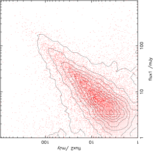
Figure 3: Distribution of flux densities for members of ‘double sources’ delineated by the combining procedure described in the text.

As a further step in identifying groups of sources that should be combined, for each ‘double source’ identified, we plotted the flux of the components against each other (Figure 3). The two fluxes are highly correlated, with most pairs lying within a narrow band about the value $flux1/flux2=1$. Such a correlation is expected for real double radio sources, for which the flux from the two lobes is correlated. Source pairs which our linking criterion does not combine show no correlation between the fluxes of the two components. This flux correlation suggests a further criterion to restrict the combination of sources to only physically associated objects: we combine pairs of sources only if their fluxes differ by a factor less than 4 (i.e. $1/4\leq\frac{flux1}{flux2}\leq 4$). Although somehow ad hoc, this upper limit on the flux ratio seems to be a reasonable guess given that it delimits a region on the $flux1-flux2$ plane that, even though quite narrow (as it has to be for physically associated objects), encloses roughly 95% of the double sources as found through equation 1. Stability of clustering measurements as a function of the collapsing procedure will be explored elsewhere.

The final number of groups obtained by including this further constraint is 17554 and their distribution as a function of number of members is shown by the dashed line in Figure 1. While keeping almost all the doubles and triples, the number of spurious groups formed by multicomponents is now reduced to a very small fraction ($<10^{-2}$) of the whole catalogue. In this way we ended up with a catalogue C3 formed by 167,433 sources.

2.3 Incompleteness

Another important issue, noted by White et al. (1997), is the incompleteness of the survey. Becker, White & Helfand (1995) estimate the catalogue to be $95\%$ complete at 2 mJy and $80\%$ complete at 1 mJy. This could affect our results in two ways. First, if there are any spatial inhomogeneities in completeness, spurious clustering will be introduced. Second, even if the incompleteness is uniform, the redshift distribution will be different from a complete flux-limited sample, and different in an unpredictable way. This difference will change the relation between 2-d and 3-d quantities, and so bias the 3-d measurements, as discussed in Section 4.

Figure 4: Differential number counts versus the integrated flux density for the three catalogues C1 (filled triangles), C2 (filled squares) and C3 (open circles), obtained from the original FIRST survey as explained in Sections 2.1 and 2.2. The dashed line shows the $\frac{dN}{dS}$ distribution as determined by Windhorst et al. (1985).

In Figure 4 we plot the differential source counts normalised to the distribution expected for a non-evolving population in Euclidean space vs the integrated flux density for the three catalogues C1 (filled triangles), C2 (filled squares) and C3 (open circles), obtained from the original FIRST survey as described in Sections 2.1 and 2.2. The dashed line shows the power-law fit to the $\frac{dN}{dS}$ distribution determined by Windhorst et al. (1985). There is a drop in the number counts for fluxes smaller that 3 mJy, and this lack of faint objects becomes very important below 2 mJy. Furthermore the summation of fluxes in the recombination of sub-components affects the incompleteness of the resulting catalogues. This is especially important in the faint-flux region. Note that as we chose an initial threshold of 1 mJy, we may lose pairs with $f_{1}+f_{2}>3$ mJy, but with either $f_{1}$ or $f_{2}$ $<1$ mJy.

From Figure 4, it is a reasonable assumption that the survey is complete at fluxes greater than 3 mJy. Hence we set a flux limit of 3 mJy for the catalogues used in our analyses. At this flux limit the C1,C2 and C3 samples contain respectively 101787, 83287 and 86074 objects. In the rest of the paper we adopt the C3 version of the catalogue, but we compare to the results with those obtained for C1 and C2.

3 CLUSTERING ANALYSIS

3.1 The Angular Two-Point Correlation Function

Correlation-function analysis has become the standard way to quantify the clustering of different populations of astronomical sources. Specifically the angular two-point correlation function $w_{12}=w(\theta)$ gives the excess probability, with respect to a random Poisson distribution, of finding two sources in the solid angles $\delta\Omega_{1}$ $\delta\Omega_{2}$ separated by an angle $\theta$, and it is defined as

$$\delta P=n^{2}\delta\Omega_{1}\delta\Omega_{2}\left[1+w(\theta)\right]$$ (2)

where $n$ is the mean number density of objects in the catalogue under consideration.

Figure 5: The angular correlation functions $w_{h}$ for C1 (open circles), C2 (open squares) and C3 (filled circles). The error bars show Poisson estimates for the C3 points. The lines show $w$ measurements from Cress et al. (1996): the solid line is for the raw catalogue and the dotted line for their ‘collapsed’ (component-combined) catalogue.

We measured $w$ for the three catalogues C1, C2 and C3 using various techniques. First we generated a random catalogue of positions and fluxes and selected sources above the sensitivity limit from the coverage map. Then we counted the number of distinct data-data pairs ($DD$), data-random pairs ($DR)$, and random-random pairs ($RR$) as a function of angular separation. We then measured $w$ from the three commonly-used estimators (Hamilton, 1993; Landy & Szalay, 1993; Peebles, 1980),

$$w_{h}= \frac{4DD\ RR}{DR^{2}} -1$$

$$w_{ls}= \frac{DD+RR-DR}{DR} -1$$

$$w_{dr}= \frac{2DD}{DR} -1$$ (3)

We also counted the number of sources in equal-area cells as discussed in section 3.2 and estimated $w$ from the cell counts,

$$w_{cell}=\frac{\langle N_{1}N_{2}\rangle}{\langle N_{1}\rangle\langle N_{2}\rangle}-1$$ (4)

For all catalogues, $w_{ls}$ and $w_{h}$ were essentially identical, and not significantly different from $w_{cell}$. The estimate $w_{dr}$ agrees perfectly on scales $\theta\mathrel{\hbox to0.0pt{\lower 3.0pt\hbox{$\sim$}\hss}\raise 2.0pt\hbox{$<$}}1^{\circ}$, but is slightly lower at $\theta\mathrel{\hbox to0.0pt{\lower 3.0pt\hbox{$\sim$}\hss}\raise 2.0pt\hbox{$>$}}1^{\circ}$.

In Figure 5 we show $w_{h}$ for the three catalogues C1, C2 and C3; the error bars show Poisson estimates for the C3 points. As the distribution is clustered these estimates only provide a lower limit to the real errors (see e.g. Mo et al., 1992) that might be obtained for instance by using the bootstrap re-sampling method. More precise estimates will be given in section 3.2 when we will move on to more quantitative results.
Note that, as it will be extensively discussed later in the paper, versions of the same catalogue obtained by adopting different collapsing procedures lead to different estimates of the angular correlation function; as it can be seen by comparing the C2 measurement with those given by the analysis of the C1 and C3 catalogues, it turns out that the higher is the number of objects that have been combined together, the shallower is the slope of the corresponding $w_{h}$. In more detail the C1 measurement shows a steepening at $\theta\mathrel{\hbox to0.0pt{\lower 3.0pt\hbox{$\sim$}\hss}\raise 2.0pt\hbox{$<$}}0.02^{\circ}$ caused by the over-counting of multiple-component sources. At very small angles ($\theta\mathrel{\hbox to0.0pt{\lower 3.0pt\hbox{$\sim$}\hss}\raise 2.0pt\hbox{$<$}}0.002^{\circ}$) the amplitude drops to $-1$, as close pairs of sources become unresolved by the survey. The C2 measurement is $-1$ for $\theta<0.02^{\circ}$ because all $DD$ pairs have been removed from the catalogue by the recombining procedure. Our C2 measurement should be comparable to the $w$ estimate from Cress et al. (1996). In fact our measurements for both C1 and C2 are in very good agreement with Cress et al. (1996) for $\theta<0.1^{\circ}$, but at larger scales we find a slightly steeper slope, leading to a difference of a factor of 2 by $\theta\sim 2^{\circ}$. The discrepancy is marginally significant given the estimated errors, and is probably due to using the more recent version of the catalogue.

The C3 measurement continues approximately as a power law to the limit of the survey resolution, $\theta\sim 0.002^{\circ}$. This gives us some confidence that our multi-component recombining procedure is reliable.

3.2 Variance

The galaxy distribution function (counts in cells) gives the probability of finding $N$ galaxies in a cell of particular size and shape. In principle the counts-in-cells distribution is straightforward to compute; one divides the space into cells of a given volume (or in our case, of given area) and shape, and then counts the number of galaxies in each cell. Obviously there cannot be less than zero galaxies in a cell, but the number of objects in each cell can grow with no upper bound (unless some negative feedback process takes place).

If we define the $k$th moment of the counts as

$$\mu_{k}=\left<(N-\bar{N})^{k}\right>$$ (5)

where $\bar{N}=n\Omega$ is the mean count in the solid angle $\Omega$, it is then possible to write these moments in terms of the $n$-point correlation functions (see e.g. Peebles, 1980). The second moment of the galaxy distribution function is related to the two-point correlation function $w_{12}$ through the expression

$$\mu_{2}=\bar{N}+(\bar{N})^{2}\Psi_{2}$$ (6)

where $\bar{N}$ is the shot noise resulting from the discrete nature of the sources (Poisson noise), and

$$\Psi_{2}\equiv\frac{1}{\Omega^{2}}\int w_{12}\>d\Omega_{1}\>d\Omega_{2}$$ (7)

is the normalised variance in terms of the two-point correlation function integrated over a cell of area $\Omega$ and particular shape.

By assuming a power-law form

$$w(\theta)=A\;\theta^{1-\gamma},$$ (8)

and by considering square cells of size $\Omega=\Theta\times\Theta$ square degrees, we can evaluate the integral in equation 7 (see Totsuji & Kihara, 1969), obtaining

$$\sigma^{2}\equiv\frac{\mu_{2}-\bar{N}}{(\bar{N}/\Omega)^{2}}=\int A\>\theta^{1-\gamma}d\Omega_{1}d\Omega_{2}=A\>C_{\gamma}\Theta^{5-\gamma}$$ (9)

where $C_{\gamma}$ is a coefficient depending on $\gamma$ which can be evaluated numerically by Monte Carlo methods (see e.g. Lahav & Saslaw, 1992). It is therefore possible to use the $\sigma^{2}-\Theta$ relation to evaluate the two parameters ($A$, $\gamma$) which describe the correlation function.

Figure 6: The normalised variance $\sigma^{2}$ vs the cell size $\Theta$ for our C3 catalogue of the FIRST survey. Errors are estimated from the variance in four random subsets.

To carry out our analysis we first project the coordinates of the objects in the survey onto an equal-area projection. We then divide the region into square cells of constant $x$ and $y$ in rectangular coordinates for the projection, and count the number of objects in each cell. We use the coverage map to discard all cells which are partially occupied, as described in section 2.2. The procedure is repeated for different cell sizes, from $\Delta x=\Delta y=\Theta=0.3^{\circ}$ up to $3^{\circ}$; at each cell size, the variance $\sigma^{2}$ is calculated from the estimator in equation 9.

Figure 6 shows $\sigma^{2}$ as a function of $\Theta$ for the C3 catalogue. The slope and the intercept of the plot are estimated by a least-squares procedure minimising the quantity

$$\chi^{2}(a,b)=\sum_{i=1}^{N}\left(\frac{\log(\sigma)_{i}-a-b\log(\Theta)_{i}}{\Delta_{i}}\right)^{2}$$ (10)

with $b\equiv(5-\gamma)$, $a\equiv\log(AC_{\gamma})$. The errors $\Delta_{i}$ are obtained using the ‘partition bootstrap method’ in which the normalised variance is calculated for four subdivisions of the survey region and the standard deviation of these measurements at each angle is used as a measure of the error. Note that this is not strictly a $\chi^{2}$ statistic, since the individual points are not independent. From this analysis we find

$$\gamma=2.50\pm 0.1\;\;\;;\;\;\;A=(1.06\pm 0.1)\cdot 10^{-3},$$ (11)

where $C_{\gamma}=6.52$ has been obtained by solving the integral in equation 9 with the condition $\theta\geq 0.01^{\circ}$, appropriate to the component-combining algorithm used to construct C3.

The amplitude $A$ is smaller by about one order of magnitude than the values obtained from optical surveys (e.g. $A=(3.82\pm 0.12)\cdot 10^{-2}$ for the APM survey (Maddox et al., 1990)); this is due to the ‘washing out’ of structure by the wide redshift span of radio surveys. The value we find for $\gamma$, high in comparison with optical surveys (e.g. $\gamma\sim 1.8$, Peebles (1980), Maddox et al. (1990)), is discussed in Section 4.

Figure 7: The normalised variance $\sigma^{2}$ vs cell size $\Theta$ for the C1 catalogue of the FIRST survey. Errors are estimated from the variance in four random subsets.

Figure 8: The normalised variance $\sigma^{2}$ vs cell size $\Theta$ for the C2 catalogue of the FIRST survey. Errors are estimated from the variance in four random subsets.

By repeating the analysis for the C1 and C2 samples (Figures 7 and 8), we find respectively:

$$\gamma=2.68\pm 0.07\;\;\;;\;\;\;A=(1.52\pm 0.06)\cdot 10^{-3}$$ (12)

and

$$\gamma=2.23\pm 0.1\;\;\;;\;\;\;A=(1.42\pm 0.1)\cdot 10^{-3}.$$ (13)

To work out the latter value of $A$, $C_{\gamma}$ has been calculated from equation 9 by imposing the condition $\theta\geq 0.02^{\circ}$, again from the nature of the component-combining criterion. The values in equation 13 are in close agreement with those obtained by Cress et al. (1996).

Comparison of the slope $\gamma$ in equations 11, 12 and 13 shows how its value decreases according to the number of source-components combined in the different catalogues ($\gamma$ largest for no combining). The presence of more ‘sources’ or ‘source components’ in close proximity, regardless of their physical association, results in a stronger correlation on smaller scales.

3.3 Skewness

Further information on clustering is contained in the higher moments of the distribution, such as the skewness and the kurtosis. Assuming Gaussian primordial perturbations and linear theory, both the skewness and the kurtosis remain zero (Peebles, 1980). A detection of a non-zero value for these quantities may then be evidence of non-linear gravitational clustering. Departures from Gaussian distributions might also reflect non-Gaussian initial conditions predicted in some cosmogonies such as cosmic-string and texture models. Detection of non-zero values for skewness and kurtosis is therefore of fundamental importance.

Kurtosis is not considered here because its estimated value is dominated by noise. Skewness is actually observed in each of the catalogues C1, C2 and C3 under consideration, starting from angles $\Theta\sim 1^{\circ}$. As seen in Figure 9, the galaxy distribution functions are noticeably skewed towards larger values of source-numbers, the tail becoming increasingly prominent as the cell-size becomes smaller. To illustrate, Figure 10 shows the comparison between sample C3 and a Poisson distribution. K-S tests show that the probabilities that the histograms are consistent with Poisson distributions are $<0.01$%.

Figure 9: Distribution function for the FIRST survey for different cell sizes. The solid lines show the results obtained for C1, and the dotted and dashed lines are for C2 and C3 respectively. The $x$ axes have been rescaled according to $x^{\prime}=x-x_{m}$, where $x_{m}$ is the median.

Figure 10: Distribution function for the FIRST survey for different cell sizes. The solid line shows the results for sample C3 compared to a Poisson distribution (dotted line).

Using an approach similar to that described in Section 3.2, the third moment (skewness) is related to the three-point correlation function $\omega_{123}$ through the expression

$$\mu_{3}=\bar{N}+3(\bar{N})^{2}\Psi_{2}+(\bar{N})^{3}\Psi_{3},$$ (14)

where

$$\Psi_{3}\equiv\frac{1}{\Omega^{3}}\int\omega_{123}\>d\Omega_{1}\>d\Omega_{2}\>d\Omega_{3}$$ (15)

is the normalised skewness in terms of the three-point correlation function integrated as in equation 7.

An estimator for the normalised variance is

$$\Psi_{2}\equiv\frac{\mu_{2}-{\bar{N}}}{({\bar{N}})^{2}}=\sigma^{2}\Omega^{2}\;,$$ (16)

and an estimator for the normalised skewness is

$$\Psi_{3}\equiv\frac{\mu_{3}-{\bar{N}}-3(\bar{N})^{2}\Psi_{2}}{(\bar{N})^{3}}\;.$$ (17)

It was shown (Peebles, 1980; Juszkiewicz et al., 1995; Coles & Frenk, 1991) that if the initial perturbations were Gaussian and they grew with cosmic time purely due to gravity, then in second-order perturbation theory (i.e. in the quasi-linear regime, $\delta\equiv{\delta\rho\over\rho}\sim 1$)

$$S_{3}^{*}(R)\equiv{\langle\delta^{3}\rangle_{R}\over\langle\delta^{2}\rangle^{2}_{R}}={34\over 7}-(n+3)\;,$$ (18)

where $S_{3}^{*}(R)$ is the spatial normalized skewness in randomly placed spheres of radius $R$ and $n$ is the index of the primordial power-spectrum of fluctuations. It follows that in this case the projected quantities obey $\Psi_{3}\propto(\Psi_{2})^{\alpha}$, with $\alpha=2$. For local surveys (e.g. Peebles, 1980), $\alpha=2$ is also expected from the empirical relation between the 3-point and 2-point correlation functions:

$$\zeta({\bf r}_{1},{\bf r}_{2})=Q[\xi(r_{1})\xi(r_{2})+\xi(r_{1})\xi(r_{12})+$$

$$+\xi(r_{2})\xi(r_{12})]\propto\xi^{2}(r),$$ (19)

where $\zeta({\bf r}_{1},{\bf r}_{2})$ is the spatial three-point correlation function.

Figure 11: The normalised variance $\Psi_{2}=\Omega^{2}\sigma^{2}$ vs the normalised, dimensionless skewness $\Psi_{3}$ for C3. Errors have been calculated as in Section 3.2.

Figure 12: $S_{3}$ as a function of $\Theta$ for C3, assuming $\alpha=2$. Errors are estimated as in Section 3.2.

Figure 13: The normalised variance $\Psi_{2}=\Omega^{2}\sigma^{2}$ vs the normalised, dimensionless skewness $\Psi_{3}$ for C1. Errors have been calculated as in section (3.2).

Figure 14: $S_{3}$ as a function of $\Theta$ for C1 assuming $\alpha=2$. Errors are estimated as in Section 3.2.

Figure 15: The normalised variance $\Psi_{2}=\Omega^{2}\sigma^{2}$ vs the normalised, dimensionless skewness $\Psi_{3}$ for C2. Errors have been calculated as in Section 3.2.

Figure 16: $S_{3}$ as a function of $\Theta$ for C2 assuming $\alpha=2$. Errors are estimated as in Section 3.2.

Figure 11 shows $\log(\Psi_{3})$ vs $\log(\Psi_{2})$ for angles $0.3^{\circ}\leq\Theta\leq 1^{\circ}$; a least-squares fit relates the quantities by the form

$$\Psi_{3}=S_{3}(\Theta)\;\Psi_{2}^{\alpha}$$ (20)

with $\alpha=1.9\pm 0.1$ and $S_{3}(\Theta)=9\pm 3$ and errors estimated as in Section 3.2. Therefore the value found for $\alpha$ supports the assumption of gravitational growth of perturbations from Gaussian initial conditions.

To test the constancy of $S_{3}$ as predicted by the hierarchical theory, we plot this quantity as a function of the cell size $\Theta$ on the assumption of $\alpha=2$ (Figure 12). The plot supports the hypothesis of constant $S_{3}(\Theta)=12.5\pm 1.5$.

The same analysis for the catalogue C1 (containing all sources), and C2 (generated by combining ‘sources’ only according to their separation), finds: $\alpha=2.0\pm 0.1,\;S_{3}(\Theta)=4\pm 2$; $S_{3}(\Theta)=4.7\pm 0.3$ for C1 (see Figures 13 and 14), and $\alpha=1\pm 2,\;S_{3}(\Theta)=1\pm 3$; $S_{3}(\Theta)=17\pm 5$ for C2. In this latter case the estimate of the quantities is dominated by noise (see Figures 15 and 16).

Table 1: COUNTS IN CELLS ANALYSIS RESULTS

	C1	C2	C3
$\gamma$	$2.68\pm 0.07$	$2.2\pm 0.1$	$2.50\pm 0.1$
$A$	$(1.52\pm 0.06)\cdot 10^{-3}$	$(1.4\pm 0.1)\cdot 10^{-3}$	$(1.06\pm 0.1)\cdot 10^{-3}$
$\alpha$	$2.0\pm 0.1$	$1\pm 2$	$1.9\pm 0.1$
$S_{3}(\Theta)$	$4\pm 2$	$1\pm 3$	$9\pm 3$
$S_{3}(\Theta)_{\alpha=2}$	$4.7\pm 0.3$	$17\pm 5$	$12.5\pm 1.5$

The results are highly sensitive to the process of ‘combining’ multi-component sources. Combining two or more ‘sources’ in close proximity strongly affects the distribution function in two ways. It removes the tail, thereby reducing skewness, and at the same time it reduces the variance as more cells will contain numbers close to the average of the distribution. The effects become rapidly more important as the number of combined sources increases; this explains the remarkable difference in the values obtained from the three catalogues. In particular the results for the C2 catalogue show that the variance and the skewness of its distribution become so small as to be dominated by noise. Note that the differences between C2 and C3 are due to less than 3000 ‘objects’ ($\sim 4\%$).

Table 1 summarises the results obtained from the counts-in-cells analysis for the three catalogues C1, C2 and C3.

4 RELATION TO SPATIAL QUANTITIES

4.1 The Spatial Correlation Function

Once both the cosmological model and the selection function of the sample are specified, the standard way of relating the spatial ($3d$) correlation function $\xi(r,z)$ to the angular ($2d$) one $w(\theta)$ is via the relativistic Limber equation (Peebles, 1980). For Einstein-de Sitter universe ($\Omega=1,\Lambda=0$),

$$w(\theta)=2\>\frac{\int_{0}^{\infty}\int_{0}^{\infty}x^{4}\Phi^{2}(x)\xi(r,z)dx\>du}{\left[\int_{0}^{\infty}x^{2}\Phi(x)dx\right]^{2}},$$ (21)

where $x$ is the comoving coordinate

$$x=\frac{c}{2H_{0}}\left[1-(1+z)^{-1/2}\right],$$ (22)

and the selection function $\Phi(x)$ satisfies the relation

$${\cal N}=\int_{0}^{\infty}\Phi(x)x^{2}dx=\frac{1}{\Omega_{s}}\int_{0}^{\infty}N(z)dz,$$ (23)

in which $\cal N$ is the mean surface density on a surface of solid angle $\Omega_{s}$ and $N(z)$ is the number of objects in the given survey within the shell ($z,z+dz$).

If we assume for $\xi(r,z)$ a power-law redshift-dependent form

$$\xi(r,z)=\left(\frac{r}{r_{0}}\right)^{-\gamma}(1+z)^{-(3+\epsilon)},$$ (24)

$\gamma$ constant with $z$, where $r$ is the proper coordinate, $r_{0}$ the correlation scale length at redshift $z=0$ and $\epsilon$ a parameter describing the redshift evolution of the spatial correlation function, then, in comoving coordinates $r_{c}=r(1+z)$, $\xi$ assumes the form

$$\xi(r,z)=\left(\frac{r_{c}}{r_{0}}\right)^{-\gamma}(1+z)^{\gamma-(3+\epsilon)}.$$ (25)

Specific values for $\epsilon$ have the following significance: $\epsilon=0$ implies constant clustering in proper coordinates; $\epsilon=\gamma-3$ implies constant clustering in comoving coordinates; and $\epsilon=\gamma-1$ represents growth of clustering under linear theory (Peebles, 1980; Treyer & Lahav, 1996).

In the small-angle approximation $r\simeq(u^{2}+x^{2}\theta^{2})^{1/2}/(1+z)$ we then find that the amplitude A defined in equations 8 and 9 is given by the expression (e.g. Loan et al., 1997; Peebles, 1980):

$$A=\left(\frac{r_{0}H_{0}}{c}\right)^{\gamma}2^{1-\gamma}\frac{\Gamma\left(\frac{1}{2}\right)\Gamma\left(\frac{\gamma-1}{2}\right)}{\Gamma\left(\frac{\gamma}{2}\right)}\times$$ (26)

$$\times\frac{\int_{0}^{\infty}\left[1-(1+z)^{-1/2}\right]^{1-\gamma}N^{2}(z)(1+z)^{\gamma-\frac{3}{2}-\epsilon}dz}{\left[\int_{0}^{\infty}N(z)dz\right]^{2}}$$

where $\Gamma$ is the Gamma function. This expression, considering the functional form (8) for $w(\theta)$, directly fixes the value of $r_{0}$ once the evolution parameter $\epsilon$ is given.

4.2 The Spatial Skewness

An analysis analogous to that in Section 4.1 provides the 3-dimensional value for the skewness $S_{3}^{*}(R)$ in randomly-placed spheres of comoving radius $R$. This is related to the projected (2-dimensional) quantity $S_{3}(\Theta)$, in the case of circular cells of radius $\theta$, through the equation (Gaztañaga, 1995)

$$S_{3}(\Theta)=r_{3}S_{3}^{*}(R)\left(\frac{C_{3}}{B_{3}}\right)$$ (27)

where $C_{3}\simeq 1$ and $B_{3}\simeq 1$ (see Gaztañaga 1994 for further details), and $r_{3}$ can be expressed as

$$r_{3}=\frac{I_{1}I_{3}}{I^{2}_{2}},$$ (28)

with

$$I_{k}=\int_{0}^{\infty}x^{2}dx\Phi^{k}x^{(3-\gamma)(k-1)}(1+z)^{(3+\epsilon-\gamma)(1-k)},$$ (29)

$\Phi(x)$ being defined by equation 23.

4.3 The redshift distribution $N(z)$

To obtain both the spatial correlation function and the spatial skewness from the respective projected quantities, we need $N(z)$, the redshift distribution for radio sources.

Figure 17: Redshift distribution N(z) for the radio source population at 1.4 GHz at a flux limit of 3 mJy. The dotted curves represent the 6 models (1-4, 6-7) taken from Dunlop & Peacock (1990); the solid curve is the average.

Figure 18: Redshift distribution N(z) for the radio source population at 1.4 GHz at a flux limit of 3 mJy. The dotted lines are models 6 and 7 from Dunlop & Peacock (1990); the solid line is the average.

There is not even a completely-identified sample of radio sources at 3 mJy, leave alone one with measured redshifts. However, the Dunlop & Peacock (DP, 1990) models of epoch-dependent luminosity functions for radio sources can be used to make estimates of $N(z)$. These models were derived with Maximum Entropy analysis to determine the coefficients for polynomial expansions to represent the epoch-dependent luminosity function; the approach incorporated the then-available identification and redshift data for complete samples from radio surveys at several frequencies. From this we have adopted three different models of $N(z)$ for subsequent deprojection analysis.

The first model ($N_{1}(z)$) is shown in Figure 17. The dotted lines represent the six models (1-4, 6-7) taken from DP and the solid line, the average, is our $N_{1}(z)$. The large spread indicates the uncertainty due to incomplete or statistically-limited redshift data as well as the extrapolation of the data to such a low flux density. Nevertheless there are two interesting features which are general. The spike seen at small redshifts indicates that at such low flux densities, the lowest-power tail of the local radio luminosity function begins to contribute substantial numbers of low-redhift sources. This spike is almost certainly underestimated; the DP analysis did not encompass the evolving starburst-galaxy population (e.g. Windhorst et al., 1985) now believed to constitute a majority of sources at mJy levels (see Wall, 1994 for an overview). The second feature is the prominent maximum around $z\sim 1$ displayed by all models, confirming that the median redshift for radio sources in radio surveys over a wide flux-density range is a factor of 10 higher than that of wide-field optical surveys.

The second model ($N_{2}(z)$) considered for our deprojections is represented by the solid line in Figure 18 and is obtained by averaging models 6 and 7 from DP, models of pure luminosity evolution. The more prominent spike at low redshifts may be a more realistic representation of the total population.

The third model ($N_{3}(z)$) is simply from $N_{1}(z)$ with the small-$z$ spike patched out.

We take $N_{1}(z)$ as our best estimate, and use $N_{2}(z)$ and $N_{3}(z)$ to test how sensitive the deprojection is to the form of $N(z)$. In particular we wish to see how the results for the correlation length $r_{0}$ and the quantity $r_{3}$ in equation 28 are affected by “extreme” models (one dominated by the spike and one completely without it).

4.4 The Predicted Angular Correlation Function

The values obtained for the slope $\gamma$ in Section 3.2 are high compared to the canonical value of 1.7 measured for optically-selected galaxies. This may be due to the intrinsic clustering properties of radio galaxies, but in this section we consider another possibility. The depth of the survey, $z\sim 1$, means that the angular scales $0.3^{\circ}<\theta<3^{\circ}$, where we measure clustering, correspond to linear scales large enough such that the correlation function $\xi(r,z)$ is no longer a simple power-law, but has steepened from that given by $\gamma\simeq 1.7$.

Figure 19: CDM prediction for the correlation function with $\Gamma=0.2$. The $y$ axis is the absolute value of $\xi(r)$. For $r\sim 100h^{-1}$ Mpc, $\xi(r)$ becomes negative, and we plot its absolute value as the dotted line.

Figure 20: CDM predictions for $w(\theta)$, showing the effects of varying the cosmological parameters, with $N(z)\equiv N_{1}(z)$ as described in Section 4.3. The dotted line is for $\Omega=1$, $h=1$, the solid line for $\Omega=0.3$, $h=0.65$, and the dashed line for $\Omega=0.5$, $h=0.5$.

If this is the case, choice of which value of $\gamma$ to use in the deprojections of equations 26 and 27 is not straightforward. We have measured the slope $\gamma=2.50$ at large scales (Section 3.2), but simply using the same slope for all scales would lead to an overestimate of $w(\theta)$ and therefore of $\xi(r,z)$ (through equation 21) at small scales. Both $r_{0}$ and $r_{3}$ are very sensitive to $\gamma$ (see below) and therefore the assessment of its proper value is very important for our conclusions.

To investigate what values are expected for $\gamma$ we have taken a theoretical correlation function $\xi(r,z)$ up to scales $r\sim 1000h^{-1}$ Mpc and projected it to get $w(\theta)$ by directly integrating equation 21. By doing the integrations numerically we do not make the assumption that $\xi$ is a power law, and do not use any of the approximations used in Section 4.1. In Figure 19 we plot the $\xi(r)$ used. On large scales it is the linear prediction for a CDM model with $\Gamma=0.2$. On small scales the linear-theory prediction underestimates the true amplitude, and as a rough approximation to allow for this, we simply extrapolated a power-law of slope $-1.7$ for scales $r<10h^{-1}$ Mpc, as observed from the APM correlation function (Maddox et al., 1990). Given the simple heuristic aims of this section, and the large uncertainties in the evolution of galaxy clustering and bias, more sophisticated methods to account for non-linearity (e.g. Peacock & Dodds, 1996) are unnecessary, though we intend a more careful study in a future paper. The overall normalization is set so that $r_{0}=5.4h^{-1}$ Mpc.

Given this form for $\xi(r)$, the shape and the amplitude of $w(\theta)$ still depend on the functional form of $N(z)$ and the values of $\Omega$, $h$. Figure 20 shows $w(\theta)$ obtained using the redshift distribution $N_{1}(z)$ as introduced in Section 4.3, with three different sets of cosmological parameters. The curves are significantly different, but they all show the same power-law behaviour for small angles, with a slope of $\sim-0.7$, corresponding to the expected $(1-\gamma)$ with $\gamma=1.7$; then, at $\theta\sim 0.3^{\circ}$, there is a break from this power law towards steeper slopes, corresponding to $\gamma\sim 3.5$ for $\theta\mathrel{\hbox to0.0pt{\lower 3.0pt\hbox{$\sim$}\hss}\raise 2.0pt\hbox{$>$}}2^{\circ}$.

In the interval $0.3^{\circ}\la\theta\la 3^{\circ}$ the curves are close to a power-law with slope $\simeq-1.5$. This is in agreement with the value of $\gamma\approx 2.5$ obtained in Section 3.2. The smaller the value of $\Omega$, the steeper is the effective slope. Of the three curves in the range $0.3^{\circ}\la\theta\la 3^{\circ}$, that for $\Omega=0.3$ and $h=0.65$ fits the data best. However this rather superficial analysis assumes a fixed $\xi(r)$ and $N(z)$, both of which will significantly change the shape of $w$. We intend to make a more thorough comparison between models and the data in a future paper.

4.5 Results

We now estimate the correlation length $r_{0}$ and the spatial normalized skewness $S_{3}^{*}(R)$ using equations 26, 27, 28 and 29 with different redshift distributions, and a range of values for $\gamma$ and $\epsilon$. We confine attention to our most reliable clustering estimates, namely those obtained in Section 3.2 from the C3 catalogue.

Figure 21: Correlation length $r_{0}$ and $r_{3}\sim S_{3}(\Theta)/S_{3}^{*}(R)$ as a function of the evolution parameter $\epsilon$ for different values of $\gamma$ and respectively $N_{1}$, $N_{2}$, $N_{3}$, in the case of the C3 catalogue; the solid line corresponds to to $\gamma=1.8$, the dotted line to $\gamma=2.0$, the short-dashed line to $\gamma=2.2$, and the long-dashed line to $\gamma=2.50$.

Figure 21 shows the trends for both the correlation length $r_{0}$ and the quantity $r_{3}$, as functions of the evolution parameter $\epsilon$, obtained for different values of $\gamma$ and the three different models for the redshift distribution $N(z)$ introduced in Section 4.3. If we fix a value for $\gamma$ and vary the form of $N(z)$, the variations for $r_{0}$ ($\la$ 10%) are not as dramatic as those for $r_{3}$. In general, the stronger the low-redshift spike in N(z) the smaller the value obtained for the correlation length $r_{0}$. If instead we fix the functional form for $N(z)$, varying $\gamma$ strongly affects both $r_{0}$ and $r_{3}$. Note also that the value of the amplitude $A$ used in the deprojection equation 26 to obtain the correlation length $r_{0}$ also depends on $\gamma$ through the quantity $C_{\gamma}$ (equation 9).

Armed with these results we face choosing the value for $\gamma$ to provide the best estimates for $r_{0}$ and $r_{3}$. Our counts-in-cells analysis carried out for scales $\Theta\leq 0.3^{\circ}$ is dominated by the shot (Poisson) noise, so we must consider clustering on larger scales. For $0.3^{\circ}\leq\Theta\leq 3^{\circ}$ we observe a slope $\gamma=2.50$ but from Section 4.4 it follows that clustering on these angular scales is determined by the spatial correlation function on scales larger than $10h^{-1}$ Mpc where a power law is not a good approximation. As mentioned in section 4.4, using $\gamma=2.50$ in equation 8 will overestimate $w(\theta)$, and hence $\xi(r)$ at small scales where the spatial correlation function is noticeably greater than 1 (see Figure 19). This will severely bias the value of $r_{0}$ obtained from integrating equation 26. This problem is even worse when we try to deproject the skewness, for the quantity $r_{3}$ appearing in equation 28 depends on the square of the correlation function (see Section 3.3). The choice of $\gamma$ is further complicated by the fact that $N(z)$ suggests the presence of at least two populations of radio sources, which may well have different clustering properties. Yet another uncertainty is introduced by fact that $\gamma$ may well be a function of redshift, even for a single population.

For convenience of comparison with other studies we quote our estimates using the “standard value” $\gamma=1.8$ and assume stable clustering ($\epsilon=0$). Adopting $S_{3}(\Theta)=12.5$, we then find

$$N_{1}(z):\;\;\;\;\;r_{0}\sim 9.7h^{-1}Mpc;\;\;S_{3}^{*}(R)\simeq\frac{S_{3}(\Theta)}{r_{3}}\sim 4.2,$$

$$N_{2}(z):\;\;\;\;\;r_{0}\sim 9.7h^{-1}Mpc;\;\;S_{3}^{*}(R)\simeq\frac{S_{3}(\Theta)}{r_{3}}\sim 1.2,$$

$$N_{3}(z):\;\;\;\;\;r_{0}\sim 10.9h^{-1}Mpc;\;\;S_{3}^{*}(R)\simeq\frac{S_{3}(\Theta)}{r_{3}}\sim 8.9.$$

(30)

We note that the values for $r_{0}$ are little affected by the choice of $N(z)$. Our estimate of $r_{0}$ for radio sources is larger than the value for optical ($r_{0}\sim 5h^{-1}$ Mpc) and IRAS galaxies ($r_{0}\sim 4h{-1}$ Mpc) and smaller than for the cluster-cluster correlation length ($r_{0}\sim 14-20h^{-1}$ Mpc).

On the other hand, we see that the spatial normalized skewness $S_{3}^{*}(R)$ is sensitive to $N(z)$. (We have neglected the small corrections for the difference between square and circular cells.) Apart from the observational uncertainties in estimating $S_{3}^{*}(R)$ for the radio sources, we should remember that comparison with the theoretical value of $S_{3}^{*}(R)$ for the mass perturbations (equation 18) depends on how radio galaxies are biased relative to the mass distribution. This bias may also be epoch-dependent (e.g. Fry, 1996). Nevertheless, our estimates are in accord with the prediction (equation 18) of $S_{3}^{*}(R)\sim 2.9$ for power-spectrum $P(k)\sim k^{-1}$ expected (based on other observations and models) on the weakly non-linear scales $R\sim 5-15h^{-1}$ Mpc probed by our analysis. (Note that angular scale of 1 degree at the median redshift of the survey, ${\bar{z}}\sim 1$, corresponds to comoving distance of $30h^{-1}$ Mpc for an Einstein - de Sitter universe.) It is also interesting to note that our values for $S_{3}^{*}$ bracket the values derived from the optical APM survey ($S_{3}^{*}\sim 3.2$; Gaztañaga et al., 1994) and from the IRAS survey ($S_{3}^{*}\sim 2.8$; Kim & Strauss, 1998), even though the observed difference in the spatial skewness could reflect differences in clustering properties between radio sources (possible mix of more objects like bright ellipticals and starbursting galaxies) and optical or IRAS galaxies.

5 CONCLUSIONS

By investigating the distribution function (counts in cells) for radio sources of the FIRST survey, we have shown how to infer the clustering properties of host radio galaxies. We considered three different catalogues above 3 mJy, generated from the original survey by following different procedures for combining source components. Focusing on the catalogue obtained with the most sensible procedure, by relating the second moment of the distribution to the angular two-point correlation function, we find a power-law behaviour for $w(\theta)$.

From the analysis of the third moment we have shown how variance and skewness are related through the functional form $\Psi_{3}=S_{3}(\Psi_{2})^{\alpha}$ with $\alpha\simeq 2$ and $S_{3}=const$ with angular scale. By inverting the projected quantities we have estimated the spatial correlation length $r_{0}\sim 10h^{-1}$Mpc and the spatial skewness $S^{*}_{3}(R)\sim 1-9$. While the value for $r_{0}$ is relatively independent of the functional form of the redshift distribution $N(z)$, the value for skewness is strongly dependent on it.

Our results indicate that the large-scale clustering of radio sources is in accord with the gravitational instability picture for the growth of perturbations from a primordial Gaussian field. Our measurements of deviations from a Gaussian distribution do not seem to require initial non-Gaussian perturbations (e.g. cosmic strings or texture).

There are crucial observations required to further this analysis. We need a better understanding of populations and source structures at mJy levels to remove statistical uncertainties due to multi-component sources. Even more important is the observational measurement of N(z), from identifications and redshift measurements for a complete sample. Radio morphologies and optical studies for a small flux-limited sample would achieve both goals.

ACKNOWLEDGEMENTS
MM acknowledges support from the Isaac Newton Scholarship. We thank Catherine Cress, George Efstathiou and David Helfand for helpful discussions.

References

- [Baleisis et al. 1998] Baleisis A., Lahav O., Loan A.J. & Wall J.V., 1998; MNRAS, in press
- [Becker et al. 1995] Becker R.H., White R.L., Helfand D.J., 1995; ApJ, 450, 559
- [Benn & Wall 1995] Benn C.R., Wall J.V., 1995; MNRAS, 272, 678
- [Coles et al. 1991] Coles P., Frenk C.S., 1991; MNRAS, 253, 727
- [Cress et al. 1996] Cress C.M., Helfand D.J., Becker R.H., Gregg M.D., White R.L., 1996; ApJ, 473, 7
- [Dunlop J.S., Peacock J.A.1990] Dunlop J.S., Peacock J.A., 1990; MNRAS, 247, 19
- [Fisher et al. 1993] Fisher K.B., Davis M., Strauss M.A., Yahil A., Huchra J.P., 1993; ApJ, 402, 42
- [Frieman & Gaztañaga 1994] Frieman J.A., Gaztañaga E., 1994; ApJ, 425, 392
- [Fry 1996] Fry J., 1996; ApJ, 461, L65
- [Fry & Gaztañaga 1993] Fry J.N., Gaztañaga E., 1993; ApJ, 413, 447
- [Gaztañaga 1994] Gaztañaga E., 1994; MNRAS, 268, 913
- [Gaztañaga 1995] Gaztañaga E., 1995; ApJ, 454, 561
- [Gaztañaga & Bernardeau 1997] Gaztañaga E., Bernardeau F., 1997; Astro-ph/9707095
- [Gregory 1991] Gregory P.C., Condon J.J., 1991; ApJS, 75, 1011
- [Griffith 1993] Griffith M.R., Wright A.E., 1993; AJ, 105, 1666
- [Hamilton 1993] Hamilton A.J., 1993; ApJ, 417, 19
- [Juszkiewicz et al. 1995] Juszkiewicz R., Weinberg D.H., Amsterdamski P., Chodorowski M., Bouchet F.R., 1995; ApJ, 42, 39
- [Kaiser 1984] Kaiser N., 1984; ApJ, 284, L9
- [Kim & Strauss1998] Kim R.S.J., Strauss M.A., 1998; ApJ, 493, 39
- [Kooiman et al. 1995] Kooiman L.K., Burns J.O., Klypin A.A., 1995; ApJ, 448, 500
- [Lahav et al. 1992] Lahav O., Saslaw W.C., 1992; ApJ, 396, 430
- [Landy & Szalay1993] Landy S.D., Szalay A.S., 1993; ApJ, 412, 64
- [Limber 1953] Limber D.N., 1953; ApJ, 117, 134
- [Loan et al. 1997] Loan A.J., Wall J.V., Lahav O., 1997; MNRAS, 286, 994
- [Maddox et al. 1990] Maddox S.J., Efstathiou G., Sutherland W.J., Loveday J., 1990; MNRAS, 242, 43P
- [Mo et al. 1992] Mo H.J., Jing Y.P., Borner G., 1992; ApJ, 392, 452
- [Oort 1987] Oort M.J.A., 1987; PhD Thesis, Leiden Observatory
- [Peacock and Dodds1996] Peacock J.A., Dodds S.J., 1996; MNRAS, 280, L19
- [Peebles 1980] Peebles P.J.E., 1980; The Large-Scale Structure of the Universe, Princeton University Press
- [Seldner 1981] Seldner M., Peebles P.J.E., 1981; MNRAS, 194, 251
- [Shaver et al. 1989] Shaver P.A., Pierre M., 1989; A&A, 220, 35
- [Sicotte 1995] Sicotte H, 1995; PhD thesis, Princeton University
- [\citemnameTotsuji et al.1969] Totsuji H., Kihara T., 1969; PASJ, 21, 221
- [\citemnameTreyer M.A., Lahav, O.1996] Treyer M.A., Lahav O., 1996; MNRAS, 280, 469
- [Wall1994] Wall J.V., 1994; Austr. J. Phys., 47, 625
- [Webster 1976] Webster A., 1976; MNRAS, 175, 61
- [White et al. 1997] White R.L., Becker R.H., Helfand D.J., Gregg M.D., 1997; ApJ, 475, 479
- [Windhorst et al.1985] Windhorst R.A., Miley G.K., Owen F.N., Kron R.G., Koo R.C., 1985; ApJ, 289, 494