Semi-Analytic Modelling of Galaxy Formation: The Local Universe

Abstract

Using semi-analytic models of galaxy formation, we investigate galaxy properties such as the Tully-Fisher relation, the B and K-band luminosity functions, cold gas contents, sizes, metallicities, and colours, and compare our results with observations of local galaxies. We investigate several different recipes for star formation and supernova feedback, including choices that are similar to the treatment in Kauffmann, White & Guiderdoni (1993) and Cole et al. (1994) as well as some new recipes. We obtain good agreement with all of the key local observations mentioned above. In particular, in our best models, we simultaneously produce good agreement with both the observed B and K-band luminosity functions and the I-band Tully-Fisher relation. Improved cooling and supernova feedback modelling, inclusion of dust extinction, and an improved Press-Schechter model all contribute to this success. We present results for several variants of the CDM family of cosmologies, and find that models with values of $\Omega_{0}\simeq 0.3$–$0.5$ give the best agreement with observations.

1 Introduction

Over the past decade and a half, a great deal of progress towards a qualitative understanding of galaxy properties has been made within the framework of the Cold Dark Matter (CDM) picture of structure formation (e.g., [Blumenthal et al. (1984)]). However, N-body simulations with gas hydrodynamics still have difficulty reproducing the observed properties of galaxies in detail (cf. [Steinmetz (1997)]). It is apparent that there must be additional physics that needs to be included in order to obtain realistic galaxies in the CDM framework. It is likely that many processes (e.g. cooling, star formation, supernova feedback, etc.) form a complicated feedback loop. It is not computationally feasible to include realistic physics over the required dynamic range in N-body simulations of significant volume, especially because we do not currently understand the details of these processes.

Semi-analytic models (SAMs) of galaxy formation are embedded within the framework of a CDM-like initial power spectrum and the theory of the growth and collapse of fluctuations through gravitational instability. They include a simplified yet physical treatment of gas cooling, star formation, supernova feedback, and galaxy merging. The Monte-Carlo approach enables us to study individual objects or global quantities. Many realizations can be run in a moderate amount of time on a workstation. Thus SAMs are an efficient way of exploring the large parameter space occupied by the unknowns associated with star formation, supernova feedback, the stellar initial mass function, metallicity yield, dust extinction, etc. However it is not only a question of computational efficiency: the macroscopic picture afforded by the semi-analytic method provides an important level of understanding that would be difficult to achieve by running an N-body simulation, even if we had an arbitrarily large and fast computer.

The semi-analytic approach to galaxy formation was formulated in ?), but this approach was not Monte-Carlo based and thus could only predict average quantities. The Monte-Carlo approach was primarily developed independently by two main groups, which we shall refer to as the “Munich” group [Kauffmann et al. (1993), Kauffmann et al. (1994), Kauffmann (1995), Kauffmann (1996a), Kauffmann (1996b), Kauffmann et al. (1997), Kauffmann & Charlot (1996)] and the “Durham” group [Cole et al. (1994), Heyl et al. (1995), Baugh et al. (1996a), Baugh et al. (1996b), Baugh et al. (1997)], because the majority of the members of these groups are associated with the Max–Planck–Institut für Astrophysik in Garching, near Munich, Germany, and the University of Durham, U.K., respectively. Similar models have also been investigated by ?) and ?). This work has shown that it is possible to reproduce, at least qualitatively, many fundamental observations in the simple framework of SAMs. These include the galaxy luminosity function (LF), the Tully-Fisher relation (TFR), the morphology-density relation, cold gas content as a function of luminosity and environment, and trends of galaxy colour with morphology and environment. However, some unsolved puzzles remain. A fundamental discrepancy has been the inability of the models to simultaneously reproduce the observed Tully-Fisher relation and the B-band luminosity function in any CDM-type cosmology [Kauffmann et al. (1993), Cole et al. (1994), Heyl et al. (1995)]. Another problem, thought to be generic to the hierarchical structure formation scenario, is the tendency of larger (more luminous) galaxies to have bluer colours than smaller (less luminous) ones, in contrast to the observed trend. We shall discuss these and other problems in detail in this paper.

This paper has several goals. We describe the ingredients of our models and show that they reproduce fundamental observations of the local universe. We repeat the calculations of several quantities that have been studied before using SAMs, and one might wonder why this is worthwhile. First, this will serve as a reference point for future papers in which we will use these models to study new problems. Second, the previous studies have been spread out over several years with different quantities being presented in different papers. Over this time the models themselves have evolved. We therefore think it will be useful to have all of these results presented in the same place in a homogeneous manner. In addition, the two main groups have not always studied the same quantities, and when they have, they have not always presented their results in a way that is directly comparable. This makes it difficult for the non-expert to judge just how different these two approaches really are. Moreover, because the models differ in so many details, it is impossible to determine which particular ingredients are responsible for certain differences in the results. Two of the important differences that we are particularly interested in are the parameterization of star formation and supernova feedback. We shall investigate the results of varying these recipes while keeping the other ingredients fixed. We also include some physical effects that have previously been neglected, and show that some of the problems that have plagued previous models can be alleviated. We investigate the importance of the underlying cosmology by examining the same quantities in a wide range of different cosmologies, spanning currently popular variants of the Cold Dark Matter (CDM) family of models.

The structure of the paper is as follows. In Section 2 we describe the basic physical ingredients of the models and briefly summarize the SAM approach. In Section 3, we summarize the model parameters and describe how we set them. In Section 4, we illustrate the effects of varying the free parameters and the star formation and supernova feedback recipes, using the properties of galaxies within a “Local Group” sized halo as an illustration. In Section 5, we present the results of our models for fundamental global quantities and galaxy properties, illustrate the effects of different choices of star formation and supernova feedback recipes on these quantities, and compare our results with previous work. We summarize and discuss our results in Section 6.

2 Basic Ingredients

In this section we summarize the simplified but physical treatments of the basic physics used in our SAMs. This includes the growth of structure in the dark matter component, shock heating and radiative cooling of hot gas in virialized dark matter halos, the formation of stars from the cooled gas, the reheating of cold gas by supernova feedback, the evolution of the stellar populations, and mergers of galaxies within the dark matter halos. There are many assumptions implicit in this modelling and in addition to describing the choices we have adopted in our fiducial models, we also remark upon some relevant details of the assumptions made in previously published work.

Our models have been developed independently, but very much in the spirit of ?, hereafter KWG93), ?, hereafter CAFNZ94), and subsequent work by these groups. We refer the reader to this literature for a more detailed introduction to the SAM approach, which here is summarized rather briefly. A more detailed review of the literature and description of an earlier version of our models is given in ?).

2.1 Cosmology

Most of the previous SAM work has been in the context of standard cold dark matter (SCDM), $\Omega_{0}=1$, $H_{0}=50\,\mbox{km s${}^{-1}$ Mpc${}^{-1}$}$, $\sigma_{8}=0.67$. However, this model has now been discredited many times in many different ways. Particularly relevant to our work is the problem that this model overproduces objects on galaxy scales relative to cluster scales. In addition the normalization $\sigma_{8}=0.67$ is highly inconsistent with the COBE data, which requires $\sigma_{8}\sim 1.2$ [Górski et al. (1996)] for this model. Many alternative variants of CDM have been suggested. We have chosen illustrative examples of popular variants of the CDM family of models, spanning the observationally plausible range of parameter space.

Table 2: Parameters of Cosmological Models. From left to right, the tabulated quantities are: the matter density, the density in the form of a cosmological constant in units of the critical density, the Hubble parameter, the baryon density in units of the critical density, the age of the universe in Gyr, the slope of the primordial power spectrum, and the linear rms mass variance on a scale of $8\mbox{$h^{-1}$ Mpc}$.

Model	$\Omega_{0}$	$\Omega_{\Lambda}$	$h$	$\Omega_{b}$	$t_{0}$	$n$	$\sigma_{8}$
SCDM	1.0	0.0	0.5	0.072	13.0	1.0	0.67
$\tau$CDM	1.0	0.0	0.5	0.072	13.0	1.0	0.60
$\Lambda$CDM.5	0.5	0.5	0.6	0.050	13.5	0.9	0.87
OCDM.5	0.5	0.0	0.6	0.05	12.3	1.0	0.85
$\Lambda$CDM.3	0.3	0.7	0.7	0.037	13.5	1.0	1.0
OCDM.3	0.3	0.0	0.7	0.037	11.3	1.0	0.85

Figure 2: The mass function from the improved Press-Schechter model proposed by [Sheth & Tormen (1999)] divided by the standard Press-Schechter mass function. This “correction factor” is a function of redshift as well as halo mass, and here is shown for $z=0$.

We have retained the standard SCDM model for comparison with previous work, and consider one other model with $\Omega_{0}=1$, the $\tau$CDM model of ?). For our purposes, the properties of this model are very similar to other popular $\Omega=1$ models such as tilted CDM ($n\sim 0.8$) and models with an admixture of hot dark matter (CHDM; [Primack et al. (1995)]). We also consider open ($\Omega_{\Lambda}=0$) and flat $\Omega_{0}+\Omega_{\Lambda}=1$) models with $\Omega_{0}=0.3$ and $\Omega_{0}=0.5$. We have assumed a Hubble parameter $h=0.7$ for the $\Omega_{0}=0.3$ models, $h=0.6$ for the $\Omega_{0}=0.5$ models, and $h=0.5$ for the $\Omega_{0}=1$ models ($H_{0}\equiv 100h\mbox{km s${}^{-1}$ Mpc${}^{-1}$}$). For the $\Omega_{0}=0.5$ flat model, we have included a mild tilt ($n=0.9$) to better simultaneously fit the power on COBE and cluster scales. For all the models, in computing the power spectrum we have assumed the baryon fraction implied by the observations of ?), $\Omega_{\rm b}=0.019\,{\rm h^{-2}}$. All models assume $T/S=0$ (no contribution from tensor modes). We use the fitting functions of ?), modified to account for the presence of baryons using the prescription of ?), to obtain the linear power spectra and COBE normalizations. The normalization $\sigma_{8}$ is roughly consistent with the $z=0$ cluster abundance and the COBE measurement except in the case of SCDM and the $\Omega_{0}=0.3$ open model, for which we have used the cluster normalization. The parameters of the cosmologies are presented in Table 2.

2.2 Dark Matter Merger Trees

The extended Press-Schechter formalism [Bower (1991), Bond et al. (1991), Lacey & Cole (1993)] provides us with an expression for the probability that a halo of a given mass $m_{0}$ at redshift $z_{0}$ has a progenitor of mass $m_{1}$ at some larger redshift $z_{1}$. Several methods of creating Monte-Carlo realizations of the merging histories of dark matter halos (“merger trees”) using this formalism have been developed [Kauffmann & White (1993), Cole (1991), Somerville & Kolatt (1998)]. Although the agreement of the Press-Schechter model with N-body simulations is in some ways surprisingly good given the simplifications involved, recent work has emphasized that there are non-negligible discrepancies. Several authors [Gross et al. (1998), Somerville et al. (1998), Tormen (1998), Tozzi & Governato (1997)] have now reported the same results using different N-body codes and different methods of identifying halos, indicating that the problems are unlikely to be explained by numerical effects. ?) showed that for a wide variety of CDM-type models, the $z=0$ Press-Schechter mass function agrees well with simulations on mass scales $M\mathrel{\hbox{\hbox to0.0pt{\hbox{\lower 4.0pt\hbox{$\sim$}}\hss}\hbox{$>$}}}10^{14}\mbox{$M_{\odot}$}$, but on smaller scales the Press-Schechter theory over-predicts the number of halos by about a factor of 1.5 to 2. The precise factor varies somewhat depending on the cosmological model and power spectrum and the way the Press-Schechter model is implemented. However, this problem cannot be solved by adjusting the critical density for collapse, $\delta_{c,0}$. In addition, the Press-Schechter model predicts stronger evolution with redshift in the halo mass function than is observed in the simulations [Gross (1997), Somerville et al. (1998)]. ?) finds a similar behaviour when comparing the predictions of the extended Press-Schechter theory with the conditional mass function of cluster-sized halos in simulations. ?) also compared the extended Press-Schechter model with the results of dissipationless N-body simulations, and investigated how well the distribution of progenitor number and mass in the simulations agrees with that produced by the merger-tree method of ?). They found that the distributions of progenitor number and mass obtained in the merging trees, which have been deliberately constructed to reproduce the Press-Schechter model, are skewed towards larger numbers of smaller mass progenitors than are found in the simulations. This problem is endemic to any method based on the extended Press-Schechter model. However, the relative properties of progenitors within a halo of a given mass are very similar in the merger trees and the simulations. This suggests that the merger trees should provide a fairly reliable framework for modelling galaxy formation, if the overall error in the Press-Schechter mass function is corrected for. An improved version of the Press-Schechter model, which gives good agreement with simulations for a variety of cosmologies, has recently been proposed by ?). The “correction factor”, i.e. the mass function from the Sheth-Tormen model divided by the standard Press-Schechter mass function, is shown in Fig. 2.

In the merger-tree method of ?), used here, the merging history of a dark matter halo is constructed by sampling the paths of individual particle trajectories using the excursion set formalism [Bond et al. (1991), Lacey & Cole (1993)]. It does not require the imposition of a grid in mass or redshift, nor are merger events required to be binary. The redshifts of branching events (i.e. halo mergers) and the masses of the progenitor halos at each stage are chosen randomly using Monte-Carlo techniques, such that the overall distribution satisfies the average predicted by the extended Press-Schechter theory. Thus when we subsequently refer to a “realization” we mean a particular Monte-Carlo realization of the halo merging history. This is the most important stochastic ingredient in the models. In order to make the tree finite, it is necessary to impose a minimum mass $m_{\rm min}$. Although the contribution of mass from halos smaller than $m_{\rm min}$ is included, we do not trace the merging history of halos with masses less than $m_{\rm min}$, but rather assume that this mass is accreted as a diffuse component. Here we take $m_{\rm min}$ to be equal to the mass corresponding to a halo with a circular velocity of 40 km/s at the relevant redshift. We argue that galaxies are unlikely to form in halos smaller than this because the gas will be photoionized and unable to cool [Weinberg et al. (1997), Forcado-Miro (1997)].

For the prediction of global quantities, we run a grid of halo masses (typically $\sim 50$ halos from $10\,m_{\rm min}$ to $V_{c}=1500$ km/s), and weight the results with the overall number density for the appropriate mass and redshift, using the improved Press-Schecter model of ?). We run many such grids and average the results.

2.3 Gas Cooling

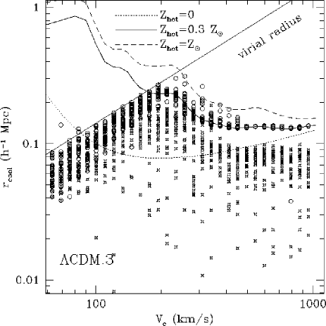
Figure 4: Cooling radius of halos as a function of circular velocity. The straight diagonal line shows the virial radius, which the cooling radius may not exceed. The curved lines show the cooling radius predicted by the literal static halo cooling model (see text), assuming that the hot gas has primordial, 0.3 solar, or solar metallicity. Open circles show the application of the static halo model within the merger trees, and crosses show the dynamic halo model (see text), assuming a fixed metallicity of 0.3 solar. Earlier conversion of gas from the hot to cold phase and reheating of hot gas by halo mergers results in a lower cooling efficiency for large halos in the dynamic halo model.

2.3.1 Cooling in Static Halos

Gas cooling is modelled using an approach similar to the one introduced by ?). We assume that each newly formed halo, at the top level of the tree, contains pristine hot gas that has been shock heated to the virial temperature of the halo ($T$) and that the gas traces the dark matter. The rate of specific energy loss due to radiative cooling is given by the cooling function $\Lambda(T)$. We can then derive an expression for the critical density which will enable the gas to cool within a timescale $\tau_{\rm cool}$:

$$\rho_{\rm cool}=\frac{3}{2}\frac{\mu m_{p}}{\chi_{e}^{2}}\frac{k_{B}T}{\tau_{\rm cool}\Lambda(T)}$$ (1)

where $\mu m_{p}$ is the mean molecular weight of the gas and $\chi_{e}\equiv n_{e}/n_{\rm tot}$ is the number of electrons per particle. Assuming that the gas is fully ionized and has a helium fraction by mass $Y=0.25$,

$$\rho_{\rm cool}=3.52\times 10^{7}\frac{k_{B}T}{\tau_{\rm cool}\Lambda_{23}(T)},$$ (2)

where $k_{B}T$ is in degrees Kelvin, $\tau_{\rm cool}$ is in Gyr, and $\Lambda_{23}(T)\equiv\Lambda(T)/(10^{-23}$ ergs s^-1 cm³). The virial temperature is approximated as $k_{B}T=71.8\sigma_{\rm vir}^{2}$, where $\sigma_{\rm vir}$ is the virial velocity dispersion of the halo. If we assume a form for the gas density profile $\rho_{g}(r)$, we can now invert this expression to obtain the “cooling radius”, defined as the radius within which the gas has had time to cool within the timescale $\tau_{\rm cool}$. For the simplified choice of the singular isothermal sphere, this gives

$$r_{\rm cool}=\left(\frac{\rho_{0}}{\rho_{\rm cool}}\right)^{1/2}$$ (3)

where $\rho_{0}=f_{\rm hot}V^{2}_{c}/(4\pi G)$, $f_{\rm hot}$ is the hot gas fraction in the cooling front and $V_{c}=\sqrt{2}\sigma_{\rm vir}$ is the circular velocity of the halo.

We use the cooling function of ?). The cooling function $\Lambda(T)$ is also metallicity dependent. In this paper, we assume that the hot gas has an average [Fe/H] = 0.3 $Z_{\odot}$ at all redshifts and for all halo masses. This value is typical of the hot gas in clusters from $z=0$ to $z\sim 0.3$ [Mushotzky & Loewenstein (1997)]. We will treat chemical enrichment in more detail and investigate the effects on cooling in a future paper. In practice, we find that the results at $z=0$ are very similar regardless of whether we use the self-consistently modelled hot gas metallicity in the cooling function, or a fixed metallicity [Fe/H] = 0.3 $Z_{\odot}$.

We divide the time interval between halo mergers (branchings) into small time-steps. For a time-step $\Delta t$, the cooling radius increases by an amount $\Delta r$ and we assume that the mass of gas that cools in this time-step is ${\rm d}m_{\rm cool}=4\pi r^{2}_{\rm cool}\rho_{g}(r_{\rm cool})\Delta r$. The cooling radius is not allowed to exceed the virial radius, and the amount of gas that can cool in a given timestep is not allowed to exceed the hot gas contained within the virial radius of the halo. For small halos, and at high redshift, the cooling is therefore effectively limited by the accretion rate. New hot gas is constantly accreted as the halo grows. When we construct the merging tree, we keep track of the amount of diffuse mass (i.e. halos below the minimal mass $m_{\rm min}$) accreted at every branching, $m_{\rm acc}$. The mass of hot gas accreted between branchings is then $f_{\rm bar}\,m_{\rm acc}$, where $f_{\rm bar}\equiv\Omega_{b}/\Omega_{0}$ is the universal baryon fraction. We assume that the mass accretion rate is constant over the time interval between branchings, which is what one would expect from the spherical collapse model (see Appendix). We also require that even if the gas is able to cool, it falls onto the disk at a rate given by the sound speed of the gas, $c_{s}=(5k_{B}T/3\mu m_{p})^{1/2}\sim 1.3\sigma_{v}$, where $\sigma_{v}$ is the 1-D velocity dispersion of the halo. Note that $c_{s}$ is approximately equal to the dynamical velocity of the halo, and that N-body simulations with hydrodynamics and cooling show that the radial infall velocity of cooling gas within the virial radius is generally close to this value [Evrard et al. (1996)].

2.3.2 Cooling and Heating in Merging Halos

In the simplest version of this approach to modelling gas cooling in dark matter halos, we imagine that a halo of a given circular velocity $V_{c}$, with a corresponding virial temperature $T$, forms at time $t=0$ and grows isothermally, gradually cooling at the rate given by the cooling function $\Lambda(T)$ as described above. In this model, the cooling time $\tau_{\rm cool}$ is the age of the Universe at the current redshift, and the gas fraction in the cooling front $f_{\rm hot}$ is always equal to the universal baryon fraction $f_{\rm bar}$. We refer to this picture as the “static halo” cooling model, as it does not account for the dynamical effects of halo mergers.

However, in the hierarchical framework of the merger trees, most halos are built up from merging halos that have experienced cooling, star formation, and feedback in previous time-steps. This modifies the gas fraction $f_{\rm hot}$ in the cooling front. The virial velocity and temperature change discontinuously following a merger, and merger events may shock heat the cooling gas. We have developed a “dynamic halo” cooling model that incorporates these effects in the following way.

For top-level halos (halos with all progenitors smaller than the minimal mass $m_{\rm min}$), the gas fraction $f_{\rm hot}$ is assumed to be equal to the universal baryon fraction $f_{\rm bar}$, and the cooling time $\tau_{\rm cool}$ is the time elapsed since the initial collapse of the halo. Subsequently, when a halo forms from the merging of two or more halos larger than $m_{\rm min}$, we determine whether the mass of the largest progenitor $m_{1}$ comprises more than a fraction $f_{\rm reheat}$ of the post-merger mass $m_{0}$. If so, the cooling radius and cooling time of the new halo are set equal to those of the largest progenitor. The gas fraction in the cooling front is taken to be $f_{\rm hot}=m_{\rm hot}/m_{\rm tot}(>r_{\rm cool})$, where $m_{\rm hot}$ is the sum of the hot gas masses of all the progenitors, and $m_{\rm tot}(r>r_{\rm cool})$ is the total mass contained between the cooling radius and the virial radius of the halo (assuming an isothermal profile). If $m_{1}/m_{0}<f_{\rm reheat}$, we assume that the hot gas within all the progenitor halos is reheated to the virial temperature of the new halo, and the cooling radius and cooling time are reset to zero. The gas fraction in the cooling front is then $f_{\rm hot}=m_{\rm hot}/m_{0}$. Note that $f_{\rm hot}$ may in principle be larger than $f_{\rm bar}$ due to reheating by supernova, but in general $f_{\rm hot}<f_{\rm bar}$ because of previous gas cooling and consumption.

We can apply the main simplifying assumptions of the static halo cooling model within the merging trees, i.e. we always assume $f_{\rm hot}=f_{\rm bar}$ and $\tau_{\rm cool}$ equal to the age of the Universe at any given time, and do not reheat the gas after any halo mergers. The results differ somewhat from the literal static halo model because we do not allow the cooling rate to exceed the available supply of hot gas, or to exceed the sound speed constraint, and because the progenitor halos cool at different temperatures. Fig. 4 shows the cooling radius in the literal static cooling model, and in the application of the static cooling model within the merging trees. For low $V_{c}$ halos, the cooling is limited by the available collapsed gas supply (i.e. $r_{\rm cool}>r_{\rm vir}$). For larger halos the results are similar to the prediction of the literal static halo model. However, the dynamic halo model (crosses) predicts significantly less cooling in large halos, due to the lower values of $f_{\rm hot}$ and the reheating by halo mergers. Note that the cooling model used by the Munich group more closely resembles the “static halo” model, and the cooling model used by the Durham group is more similar to our “dynamic halo” cooling model In this paper, we will show results for both cooling models.

2.4 Disk Sizes

To obtain a very rough estimate of the sizes of disks that form in our models, we adopt the general picture of ?), in which the gas collapse is halted by angular momentum conservation. We define $\lambda_{H}$ to be the dimensionless spin parameter of the halo, $\lambda_{H}\equiv J|E|^{1/2}G^{-1}M^{-5/2}$, where $J$ is the angular momentum, $M$ is the mass and $E$ is the energy of the dark matter halo. We assume that the gas has the same specific angular momentum as the dark matter, and collapses to form a disk with an exponential profile. For a singular isothermal halo, the scale radius of the disk that forms is then $r_{s}=1/\sqrt{2}\lambda_{H}r_{i}$, where $r_{i}$ is the radius before collapse (in our models, $r_{i}={\rm min}(r_{\rm cool},r_{\rm vir}$). We neglect the modification of the inner profile of the dark matter due to the infall of the baryons, which will tend to lead to smaller disks [Blumenthal et al. (1986), Flores et al. (1993), Mo et al. (1998)].

The distribution of $\lambda_{H}$ found in N-body simulations [Barnes & Efstathiou (1987), Kravtsov et al. (1998), Lemson & Kauffman (1997)] is a rather broad log-normal with mean $\langle\lambda_{H}\rangle=0.05$. It is likely that in order to obtain a realistic distribution of galaxy sizes and surface brightnesses, we should consider a range of values of $\lambda_{H}$ as seen in the above simulations [Dalcanton et al. (1997), Mo et al. (1998)]. However, it is not known how $\lambda_{H}$ is affected by mergers, so we do not know how to propagate this quantity through the merging trees. We should also use a more realistic halo profile than the singular isothermal sphere. We intend to address the modelling of disk sizes in more detail in the future. For the present, we use $\lambda_{H}=0.05$ for all halos.

Figure 6: The star formation rate per unit mass of cold gas (star formation efficiency) as a function of circular velocity. The solid curved line shows the Durham star formation law (SFR-D), which has no explicit dependence on redshift, and the horizontal dashed lines show the Munich star formation law (eqn. SFR-M), for $z=5,3,1,0$ from highest to lowest, respectively.

2.5 Star Formation

The star formation recipes that we will consider in this paper are of the general form

$$\dot{m}_{*}=\frac{m_{\rm cold}}{\tau_{*}},$$ (4)

where $m_{\rm cold}$ is the total mass of cold gas in the disk and we hide all of our ignorance in the efficiency factor $\tau_{*}$. The simplest possible choice is to assume that $\tau_{*}=\tau_{*}^{0}$ is constant. This would imply that once it is cold, gas is converted to stars with the same efficiency in disks of all sizes and at all redshifts. We shall refer to this recipe as SFR-C.

Another choice is a power law, in which the star formation efficiency is a function of the circular velocity of the galaxy:

$$\dot{m}_{*} = \frac{m_{\rm cold}}{\tau_{*}(V_{c})}$$ (5)

$$\tau_{*}(V_{c}) = \tau_{*}^{0}\left(\frac{V_{c}}{V_{0}}\right)^{\alpha_{*}}$$ (6)

where $m_{\rm cold}$ is the mass of cold gas in the disk, $\tau_{*}^{0}$ and $\alpha_{*}$ are free parameters, and $V_{0}=300\,\mbox{km s${}^{-1}$}$ is an arbitrary normalization factor. This is equivalent to the approach used by the Durham group, and we will refer to this recipe as SFR-D.

The other approach, used by the Munich group, assumes that the timescale for star formation is proportional to the dynamical time of the disk

$$\dot{m}_{*}=\frac{m_{\rm cold}}{\tau_{*}^{0}\,\tau_{\rm dyn}}.$$ (7)

Here $\tau_{*}^{0}$ is a dimensionless free parameter, and $\tau_{\rm dyn}$ is the dynamical time of the galactic disk, $\tau_{\rm dyn}=r_{\rm disk}/V_{c}$. Following KWG93, we take $r_{\rm disk}$ to be equal to one tenth the virial radius of the dark matter halo, and $V_{c}$ to be the circular velocity of the halo at the virial radius. For satellite galaxies, the dynamical time remains fixed at the value it had when the galaxy was last a central galaxy. We will refer to this star formation recipe as SFR-M.

It is worth noting the differences in these assumptions and the implications for the models. The dynamical time $\tau_{\rm dyn}$ at a given redshift is nearly independent of the galaxy circular velocity. This is because the spherical collapse model predicts that the virial radius scales like $r_{\rm vir}\propto V_{c}$ (see Appendix). However, the virial radius of a halo with a given circular velocity increases with time ($r_{\rm vir}\propto(1+z)^{-3/2}$ for an Einstein-de Sitter universe). This means that SFR-M is approximately constant over circular velocity but has a higher efficiency at earlier times (higher redshift). In contrast, SFR-D has no explicit dependence on redshift but does depend fairly strongly on the galaxy circular velocity ($\alpha_{*}=-1.5$ in the fiducial Durham models), so that star formation is less efficient in halos with small $V_{c}$. This is illustrated in Fig. 6. Because a “typical” halo at high redshift is less massive and hence has a smaller circular velocity in hierarchical models, this has the effect of delaying star formation until a later redshift, when larger disks start to form. SFR-M therefore leads to more early star formation. We will discuss this further in Section 4.

2.6 Supernova Feedback

2.6.1 Previous Feedback Recipes

In the Munich and Durham models, the rate of reheating of cold gas is given by

$$\dot{m}_{\rm rh}=\epsilon^{0}_{\rm SN}(V_{c}/V_{0})^{-\alpha_{\rm rh}}\dot{m}_{*}$$ (8)

where $\epsilon^{0}_{\rm SN}$ and $\alpha_{\rm rh}$ are free parameters, $\dot{m}_{*}$ is the star formation rate, and $V_{0}$ is a scaling factor chosen so that $\epsilon^{0}_{\rm SN}$ is of order unity ($V_{0}=400\,\mbox{km s${}^{-1}$}$ for the Munich models and 140 km s^-1for the Durham models). The Munich group assumes $\alpha_{\rm rh}=2$, whereas the fiducial models of the Durham group assume a considerably stronger dependence on circular velocity, $\alpha_{\rm rh}=5.5$.

The “reheated” gas is removed from the cold gas reservoir. An important issue is whether the reheated gas remains in the halo in the form of hot gas, where it will generally cool again on a short timescale, or is expelled from the potential well of the halo entirely. In the Munich models (previous to 1998), all the reheated gas is retained in the halo (G. Kauffmann, private communication). In the Durham models, all the reheated gas is ejected from the halo. This gas is then returned to the hot gas reservoir of the halo after the mass of the halo has doubled (Durham group, private communication). We find that the results of the models are quite sensitive to whether the gas is retained in or ejected from the halo. We would therefore like to find a simple but physical way of modelling the ejection of the reheated gas from the disk and the halo without introducing an additional free parameter. To this end, we have introduced the following modified treatment of supernova feedback.

2.6.2 The Disk-Halo Feedback Model

We assume that the mass profile of the disk is exponential. The potential energy of an exponential disk with scale radius $r_{s}$ and central surface density $\Sigma_{0}$ is approximately $W\simeq-11.6G\Sigma_{0}^{2}r_{s}^{3}$ [Binney & Tremaine (1987)]. We can then calculate the rms escape velocity for the disk, $\langle v^{2}_{\rm esc,\,disk}\rangle^{1/2}=\sqrt{-4W/m_{d}}$, where $m_{d}$ is the mass of the disk. Similarly, for the halo, the rms escape velocity is $\langle v^{2}_{\rm esc,\,halo}\rangle^{1/2}=\sqrt{-4W/m_{halo}}=\sqrt{2}V_{c}$, using the virial theorem. As before, we have the free parameter $\epsilon^{0}_{\rm SN}$, which we interpret loosely as the fraction of the supernova energy transferred to the gas in the form of kinetic energy. The rate at which kinetic energy is transferred to the gas is now $\dot{\epsilon}_{\rm SN}=\epsilon^{0}_{\rm SN}\,E_{\rm SN}\,\eta_{\rm SN}\,\dot{m}_{*}$, where $E_{\rm SN}=10^{51}$ ergs is the total (kinetic and thermal) energy per supernova, $\eta_{\rm SN}$ is the number of supernova per solar mass of stars ($\eta_{\rm SN}=3.2\times 10^{-3}$ for the Scalo IMF used here [Bruzual & Charlot (1993)]), and $\dot{m}_{*}$ is the star formation rate. Following the general arguments of ?), we now calculate the rate at which gas can escape from the disk:

$$\dot{m}_{\rm rh,\,disk}=2f_{\rm rh,disk}\frac{\dot{\epsilon}_{\rm SN}}{\langle v^{2}_{\rm esc,\,disk}\rangle},$$ (9)

and from the halo (same expression with $\langle v^{2}_{\rm esc,\,halo}\rangle$). The factor $f_{\rm rh,disk}$ is a fudge factor that we leave fixed to $f_{\rm rh,disk}=2$. In general, ${\rm d}m_{\rm rh,\,disk}$ is then larger than ${\rm d}m_{\rm rh,\,halo}$. The gas that can escape from the disk but not the halo is added to the hot gas in the halo. Gas that can escape from both the disk and the halo is removed from the halo entirely. Because of the uncertainties involved, we do not attempt to model the recollapse of this gas at later times, so this gas will never be re-incorporated into any halo and is “lost” forever.

2.7 Chemical Evolution

We trace chemical evolution by assuming a constant “effective yield”, or mean mass of metals produced per mass of stars. The value of the effective yield, $y$, is treated as a free parameter. We assume that newly produced metals are deposited in the cold gas. Subsequently, the metals may be ejected from the disk and mixed with the hot halo gas, or ejected from the halo, in the same proportion as the reheated gas, according to the feedback model described above. The metallicity of each batch of new stars equals the metallicity of the cold gas at that moment. Note that because enriched gas may be ejected from the halo, and primordial gas is constantly being accreted by the halo, this approach is not equivalent to a standard “closed box” model of chemical evolution. Also note that although we track the metallicity of the hot gas by this procedure, in this paper we do not use this metallicity to compute the gas cooling rate (see Section 2.3).

2.8 Galaxy Merging

2.8.1 Dynamical Friction and Tidal Stripping

When halos merge, we assume that the galaxies within them remain distinct for some time. In this way we eventually end up with many galaxies within a common dark matter halo, as in groups and clusters. The central galaxy of the largest progenitor halo becomes the new central galaxy and the other galaxies become “satellites”. Following a halo merger event, we assume that the satellites of the largest progenitor halo remain undisturbed and place the central galaxies of the other progenitors at a distance $f_{\rm mrg}r_{\rm vir}$ from the central galaxy, where $f_{\rm mrg}$ is a free parameter and $r_{\rm vir}$ is the virial radius of the new parent halo. Satellites of the other progenitors are distributed randomly around their previous central galaxy, preserving their relative distance from that galaxy. All the satellites lose energy due to dynamical friction against the dark matter background and fall in towards the new central object.

The differential equation for the distance of the satellite from the center of the halo ($r_{\rm fric}$) as a function of time is given by

$$r_{\rm fric}\frac{{\rm d}r_{\rm fric}}{{\rm d}t}=-0.428f(\epsilon)\frac{Gm_{\rm sat}}{V_{c}}\ln\Lambda$$ (10)

[Binney & Tremaine (1987), Navarro et al. (1995)]. In this expression, $m_{\rm sat}$ is the combined mass of the satellite’s gas, stars, and dark matter halo, and $V_{c}$ is the circular velocity of the parent halo. Not to be confused with at least two other quantities in this paper denoted by the same symbol, here $\ln\Lambda$ is the Coulomb logarithm, which we approximate as $\ln\Lambda\approx\ln(1+m_{h}^{2}/m_{\rm sat}^{2}$), where $m_{h}$ is the mass of the parent halo. The circularity parameter $\epsilon$ is defined as the ratio of the angular momentum of the satellite to that of a circular orbit with the same energy: $\epsilon=J/J_{c}(E)$. ?) show that the approximation $f(\epsilon)=\epsilon^{0.78}$ is a good approximation for $\epsilon>0.02$. We draw $\epsilon$ for each satellite from a uniform distribution from 0.02 to 1. A new value of $\epsilon$ is chosen if the parent halo merges with a larger halo.

As the satellite falls in, its dark matter halo is tidally stripped by the background potential of the parent halo. We approximate the tidal radius $r_{t}$ of the satellite halo by the condition $\rho_{\rm sat}(r_{t})=\rho_{\rm halo}(r_{\rm fric})$, i.e. the density at the tidal radius equals the density of the background halo at the satellite’s current radial position within the larger halo. The mass of the satellite halo can then be estimated as the mass within $r_{t}$. We assume that both halos can be represented by singular isothermal spheres, $\rho\propto r^{-2}$. When $r_{\rm fric}$ is less than or equal to the radius of the central galaxy, the satellite merges with the central galaxy.

2.8.2 Satellite-Satellite Mergers

Satellite galaxies may also collide with each other as they orbit within the halo. They may merge or only experience a perturbation depending on their relative velocities and internal velocity dispersions. From a simple mean free path argument, one expects satellites to collide on a time scale

$$\tau_{\rm coll}\sim\frac{1}{\bar{n}\sigma v}$$ (11)

where $\bar{n}$ is the mean density of galaxies, $\sigma$ is the effective cross section for a single galaxy, and $v$ is a characteristic velocity. High-resolution N-body simulations by ?) indicate that this simple scaling actually describes the merger rate quite accurately for collisions of galaxy pairs over a broad range of parameter space. They generalize their results to obtain an expression for the average time between collisions in a halo containing $N$ equal mass galaxies:

$$\tau_{\rm coll}=500\,N^{-2}\left(\frac{r_{\rm halo}}{\rm Mpc}\right)^{3}\left(\frac{r_{\rm gal}}{\rm 0.12\>Mpc}\right)^{-2}$$ (12)

$$\left(\frac{\sigma_{\rm gal}}{\rm 100\>km\,s^{-1}}\right)^{-4}\left(\frac{\sigma_{\rm halo}}{\rm 300\>km\,s^{-1}}\right)^{3}{\rm Gyr}.$$

Here $r_{\rm halo}$ is the virial radius of the parent halo, $r_{\rm gal}$ is the tidal radius of the dark matter bound to the satellite galaxy, $\sigma_{\rm gal}$ is the internal 1-D velocity dispersion of the galaxy, and $\sigma_{\rm halo}$ is the 1-D velocity dispersion of the parent halo. Although this expression was derived for equal mass galaxies, we use it to assign a collision timescale $t_{\rm coll}$ to each galaxy using the mass and tidal radius of each individual sub-halo. The probability that a galaxy will merge in a given timestep $\Delta t$ is then $P_{\rm mrg}=\Delta t/t_{\rm coll}$. A new velocity dispersion and mass is assigned to the post-merger sub-halo by assuming that energy is conserved in the collision, and that the merger product satisfies the virial relation. Note that we do not allow random collisions between satellite galaxies and central galaxies, even though they are in principle quite likely, because we do not know how to model the cross-section for such events.

2.8.3 Merger-Induced Starbursts

There is considerable observational and theoretical evidence that mergers and interactions between galaxies trigger dramatically enhanced star formation episodes known as starbursts. When two galaxies merge according to either of the two processes described above, we assume that the cold gas is converted to stars at the enhanced rate $e_{\rm burst}m_{\rm cold}/\tau_{\rm dyn}$, where $m_{\rm cold}$ is the combined cold gas of both galaxies, and $\tau_{\rm dyn}$ is the dynamical time of the larger galaxy. The burst efficiency $e_{\rm burst}$ may depend on the mass ratio of the merging galaxies, and is typically between 0.50 to 1. The mean properties of galaxies at $z=0$ are quite insensitive to the details of the treatment of starbursts, although this process turns out to be quite important for high redshift galaxies. We develop a more detailed treatment of starbursts, based on simulations with hydrodynamics and star formation [Mihos & Hernquist (1994), Mihos & Hernquist (1996)], and investigate the implications for high redshift galaxies in a seperate paper [Somerville et al. (1999)].

2.8.4 Merger-Driven Morphology

Simulations of collisions between nearly equal mass spiral galaxies produce merger remnants that resemble elliptical galaxies. Accretion of a low-mass satellite by a larger disk will heat and thicken the disk but not destroy it [Barnes & Hernquist (1992)]. However the line dividing these cases is fuzzy and depends on many parameters other than the mass ratio, such as the initial orbit, the relative inclination, whether the rotation is prograde or retrograde, etc. We introduce a free parameter, $f_{\rm bulge}$, which determines whether a galaxy merger leads to formation of a bulge component. If the mass ratio $m_{S}/m_{B}$ is greater than $f_{\rm bulge}$, then all the stars from both galaxies are put into a “bulge” and the disk is destroyed (here $m_{S}$ and $m_{B}$ are the baryonic masses of the smaller and bigger galaxy, i.e. the sum of the cold gas and stellar masses). If $m_{S}/m_{B}<f_{\rm bulge}$, then the stars from the smaller galaxy are added to the disk of the larger galaxy. The cold gas reservoirs of both galaxies are combined. Additional cooling gas may later form a new disk. The bulge-to-disk ratio at the observation time can then be used to assign rough morphological types. ?) have correlated the Hubble type and the B luminosity bulge-to-disk ratio. Using their results, and following KWG93, we categorize galaxies with $B/D>1.52$ as ellipticals, $0.68<B/D<1.52$ as S0s, and $B/D<0.68$ as spirals. Galaxies with no bulge are classified as irregulars. As shown by KWG93 and ?), this approach leads to model galaxies with morphological properties that are in good agreement with a variety of observations.

2.9 Stellar Population Synthesis

Stellar population synthesis models provide the Spectral Energy Distribution (SED) of a stellar population of a single age. These models must assume an Initial Mass Function (IMF) for the stars, which dictates the fraction of stars created with a given mass. The model stars are then evolved according to theoretical evolutionary tracks for stars of a given mass. By keeping track of how many stars of a given age are created according to our star-formation recipe, we create synthesized spectra for the composite population. A free parameter $f^{*}_{\rm lum}$ effectively determines the stellar mass-to-light ratio; $f^{*}_{\rm lum}$ is defined as the ratio of the mass in luminous stars to the total stellar mass, $m^{*}_{\rm lum}/m^{*}_{\rm tot}$. The remainder is assumed to be in the form of brown dwarfs, planets, etc. We then convolve the synthesized spectra for each galaxy with the filter response functions appropriate to a particular set of observations. In this way we obtain colours and magnitudes that can be directly compared to observations at any redshift.

Although this approach is satisfying because it results in quantities that can be compared directly to observations, there are many uncertainties inherent in this component of the modelling, as is bound to be the case with such a complicated problem. The IMF is a major source of uncertainty. The IMF is fairly well determined in our Galaxy [Scalo (1986)], but we know very little about how universal it is or whether it depends on metallicity or other environmental effects. The results are somewhat sensitive to the upper and lower mass cutoffs as well as the slope of the IMF. Then of course there are the difficulties of modelling the complex physics involved in stellar evolution. Some of the major sources of uncertainty mentioned by ?) are opacities, heavy-element mixture, helium content, convection, diffusion, mass loss, and rotational mixing. Comparing three sets of models, ?) find only a 0.05 magnitude dispersion between the models in $B-V$ colour, but a larger discrepancy of 0.25 magnitudes in $V-K$ colour and a 25% dispersion in the mass-to-visual light ratio. However, they also stress that there are far greater uncertainties involved in the modelling of young ($<1$ Gyr) stars, especially stars more massive than 2 $M_{\odot}$.

There are currently several versions of stellar population models available. We have used the Bruzual & Charlot (GISSEL95) models [Bruzual & Charlot (1993), Charlot et al. (1996)]. These models are for solar metallicity stars only. For the results presented in this paper, we have used a Scalo [Scalo (1986)] IMF and the standard Johnson filters provided with GISSEL95.

Table 4: Cooling/Merging Packages

name	cooling	merging	starbursts
Classic	static halo	dynamical friction only	major mergers only; $e_{\rm burst}=1$
New	dynamic halo	dynamical friction + satellite collisions	all mergers; $e_{\rm burst}=f(m_{1}/m_{2})$

Table 6: Star Formation/Feedback Packages

name	star formation	feedback	reheated gas
Munich	SFR-M	eqn. 8, $\alpha_{\rm rh}=2$	all stays in halo
Durham	SFR-D	eqn. 8, $\alpha_{\rm rh}=5.5$	all ejected from halo
Santa Cruz (fiducial)	SFR-M	disk/halo	disk/halo
Santa Cruz (high fb)	SFR-M	disk/halo	disk/halo
Santa Cruz (C)	SFR-C	disk/halo	disk/halo

2.10 Dust Absorption

Absorption of galactic light by dust in the interstellar medium causes galaxies to appear fainter and redder in the ultraviolet to visible part of the spectrum. In this paper, we have adopted a simple model of dust extinction based on the empirical results of ?). These authors give an expression for the B-band, face-on extinction optical depth of a galaxy as a function of its blue luminosity:

$$\tau_{B}=\tau_{B,*}\left(\frac{L_{B,i}}{L_{B,*}}\right)^{\beta}\,,$$ (13)

where $L_{B,i}$ is the intrinsic (unextinguished) blue luminoisity, and we use $\tau_{B,*}=0.8$, $L_{B,*}=6\times 10^{9}L_{\odot}$, and $\beta=0.5$, as found by ?). We then relate the B-band optical depth to other bands using a standard Galactic extinction curve [Cardelli et al. (1989)]. The extinction in magnitudes is then related to the inclination of the galaxy using a standard “slab” model (a thin disk with stars and dust uniformly mixed together):

$$A_{\lambda}=-2.5\log\left(\frac{1-e^{-\tau_{\lambda}\sec\theta}}{\tau_{\lambda}\sec\theta}\right)$$ (14)

where $\theta$ is the angle of inclination to the line of sight[Guiderdoni & Rocca-Volmerange (1987), Tully & Fouqué (1985)]. We assign a random inclination to each model galaxy. The extinction correction is only applied to the disk component of the model galaxies (i.e. we assume that the bulge component is not affected by dust).

2.11 Model Packages

There are many possible permutations of the different ingredients that we have introduced above. In the interest of practicality, we have chosen several “packages” of ingredients to explore in this paper. In the relevant sections, we comment on which elements of the package are important in determining various quantities.

In order to understand the effects of the new ingredients that we have introduced pertaining to cooling, galaxy merging, and starbursts, we introduce two “cooling/merging” packages (see Table 4). The ingredients of the “Classic” package were chosen to be similar to the published Munich and Durham models . In this paper, we always apply them within the SCDM cosmology, which was used for much of the previous work. The ingredients of the “New” cooling/merging package reflect additions or modifications to our models. We apply the “New” models within more realistic (or anyway more fashionable) cosmologies. The new ingredients are described above, namely, the dynamic-halo cooling model (Section 2.3), satellite collisions (Section 2.8), and more detailed modelling of starbursts in galaxy-galaxy mergers. In the “Classic” models, starbursts occur only in major mergers and with efficiency $e_{\rm burst}=1$. In the “New” models, starbursts occur in all mergers and $e_{\rm burst}$ is a function of the mass ratio of the merging galaxies. The details of the starburst modelling are of minor importance for galaxy properties at $z\sim 0$, and will be dealt with in detail in a companion paper [Somerville et al. (1999)].

We also wish to understand the effects of different choices of star formation and supernova feedback recipes, and introduce several “sf/fb” packages. We have chosen the ingredients of the first two packages to be similar to the choices made by the Munich and Durham groups with respect to the star formation and supernova feedback, including the fate of reheated gas (see Section 2.6). It should be kept in mind, however, that although we will refer to these as the “Munich” and “Durham” packages, our models differ from those of these other groups in many respects and we are not trying to reproduce their results in detail. On the contrary, we wish to isolate the effects of the way that star formation and supernova feedback are modelled. For example, as we will discuss in Section 3, the published models of the Munich and Durham groups are normalized such that a galaxy of a given circular velocity is considerably fainter than in our models. Here we will always normalize all of the packages in the same way, as described in Section 3. We will refer to the results that we obtain from our code, normalized as described in this paper, as the Munich and Durham “packages”. When we wish to refer to the results obtained by the Munich and Durham groups using their codes, normalized in their own ways, we shall refer to the “actual” or “published” Munich or Durham models.

The third package, which we refer to as the “Santa Cruz (fiducial)” package, is a hybrid of the Munich-style star formation law (SFR-M) and the disk-halo feedback model described in Section 2.5. “Santa Cruz (high fb)” is the same as Santa Cruz (fiducial) except that the supernova feedback parameter is turned up by a factor of five. The “Santa Cruz (C)” package assumes that the star formation efficiency is constant at all redshifts and in galaxies of all sizes (SFR-C). Note that this is equivalent to the star formation law suggested for use with milder supernova feedback ($f_{\rm v}=0.01$) by CAFNZ94. Again, we combine this with the disk-halo feedback model.

3 Setting the Galaxy Formation Parameters

We have introduced a number of parameters. “Free” parameters are adjusted for each choice of cosmology and package of astrophysical recipes, according to criteria that we shall describe. The “fixed” parameters keep the same values for all of the models. In this section, we summarize the parameters and the procedure that we use to set them.

Figure 8: Fits to the observed I-band Tully-Fisher relation from several samples. PT92 is the [Pierce & Tully (1992)] relation for nearby galaxies, scaled assuming various values of the Hubble parameter. Giovanelli et al. is from the ?) sample of cluster spirals. HM and MAT are the Han-Mould and Mathewson et al. samples discussed in Willick et al. (?, ?). The magnitude of a “Milky Way” galaxy ($V_{c}=220\,\mbox{km s${}^{-1}$}$) in the Durham models, from Fig. 11 of CAFNZ94 is indicated by the open square. The approximate magnitude of a “Milky Way” galaxy in the Munich models is indicated by the open triangle. The magnitude of the “Milky Way” in our models is indicated by the filled hexagon.

3.1 Fixed parameters

The physical meaning and values of the fixed parameters, as well as the section in which they are discussed in detail, are summarized as follows:

• $\alpha_{*}=-1.5$ (2.5): power used in power-law (Durham) star formation law

• $\alpha_{rh}$ (2.6.1): power used in supernova reheating power-law ($\alpha_{rh}=2$ for Munich, $\alpha_{rh}=5.5$ for Durham)

• $f_{\rm rh,disk}=2$ (2.6.2) : fudge factor used in disk-halo feedback model

• $f_{\rm reheat}=0.5$ (2.3.2): In the dynamic halo cooling model, the cooling time $\tau_{\rm cool}$ is reset after a halo merger event if the largest progenitor of the current halo is less than a fraction $f_{\rm reheat}$ of its mass.

• $Z_{\rm hot}$ (2.3): the assumed metallicity of the hot gas, used in the cooling function.

3.2 Free Parameters

The free parameters and the sections in which they were introduced are:

• $\tau_{*}^{0}$ (2.5): the star formation timescale

• $\epsilon^{0}_{\rm SN}$ (2.6): supernova reheating efficiency

• $y$ (2.7) : chemical evolution yield (mass of metals produced per unit mass of stars)

• $f^{*}_{\rm lum}$ (2.9): the fraction of the total stellar mass in luminous stars

• $f_{\rm mrg}$ (2.8.1): the initial distance of satellite halos from the central galaxy after a halo merger, in units of the (post-merger) virial radius.

• $f_{\rm bulge}$ (sec:models:morph): the mass ratio that divides major mergers from minor mergers; determines whether a bulge component is formed

To set the values of the free parameters, we define a fiducial “reference galaxy”, which is the central galaxy in a halo with a circular velocity of ${V_{c}=220\>\mbox{km s${}^{-1}$}}$. We set the most important free parameters by requiring the properties of this reference galaxy to agree with observations for an average galaxy with this circular velocity. As an important constraint, we would like to require our reference galaxy to have an average I magnitude given by the Tully-Fisher relationship (we normalize in I rather than B because it is less sensitive to recent starbursts and the effects of dust). But first, we discuss a subtlety in the process of comparing the models with this observation, which has led to some confusion in the past.

3.2.1 Tully-Fisher Normalization

If we use a local sample, such as that of ?), the relation between absolute magnitude and line-width has been determined by measuring a distance to each galaxy using various standard methods (e.g. Cepheids, RR Lyrae, planetary nebulae). This relation therefore intrinsically contains an effective Hubble parameter. The ?) sample, when used to derive distances to the Ursa Major and Virgo clusters, implies $H_{0}=85\pm 10\,\mbox{km s${}^{-1}$ Mpc${}^{-1}$}$ [Pierce & Tully (1988)]. Our models are set within predetermined cosmologies with various values of the Hubble parameter ($H_{0}=$ 50, 60, or 70 km s^-1 Mpc^-1). To compare this data to the different cosmologies used in our models, one approach is to simply scale the observed absolute magnitudes:

$$M_{\rm model}=M_{\rm obs}+5\log(h_{\rm model}/h_{\rm obs})$$ (15)

This is effectively what CAFNZ94 say they have done in their Fig. 11, assuming $h_{\rm obs}=1.0$ (although it looks more as though they used $h=0.80$). They then interpret their Fig. 11 as indicating that their models are discrepant with the observed Tully-Fisher relation because their galaxies are $\sim 1.8$ magnitudes too faint at a given circular velocity. In contrast, KWG93 claim good agreement with the Tully-Fisher relation, and show this in their Fig. 7. This leaves one with the impression that a Durham galaxy would be about 1.8 magnitudes fainter than a Munich galaxy with the same circular velocity.

It is difficult to make a direct comparison from the published papers because KWG93 plot the TF relation in the B band, and in terms of luminosity, whereas CAFNZ94 use the I band, and plot $M_{I}-5\log h$. However, we can easily check what would happen if we scaled the B-band relation used by KWG93 in the same way. If we assume $M_{\rm B,obs}=-20.7$ for a ${V_{c}=220\>\mbox{km s${}^{-1}$}}$ galaxy, from the ?) relation, and take $h_{\rm obs}=1.0$ and $h_{\rm model}=0.5$, this would imply $M_{\rm B,model}=-22.2$. This is 1.2 to 2.2 magnitudes brighter than the “Milky Way” normalization ($M_{B}\sim-20$ to -21), used in the published Munich models. What this means is that the apparent good agreement with the TFR seen in Fig. 7 of KWG93 is because they assumed $h_{\rm obs}=h_{\rm model}=0.5$.

Table 8: Galaxy formation parameters for the “Classic” models (SCDM)

model	$\tau^{0}_{*}$	$\epsilon^{0}_{\rm SN}$	$y$	$f^{*}_{\rm lum}$	$f_{\rm bar}$
Munich	100	0.2	1.3	1.0	0.1
Durham	4.0	N/A	1.8	1.0	0.125
Santa Cruz (fiducial)	100	0.1	1.8	1.0	0.125
Santa Cruz (high fb)	100	0.5	4.0	1.0	0.125
Santa Cruz (C)	8.0	0.125	1.8	1.0	0.125

One lesson in all of this is that trying to normalize the models with the local Tully-Fisher data is problematic because it is so sensitive to the Hubble parameter. A more robust approach is to use the velocity-based zero-point from the compilation of several more distant TF samples from Willick et al. (?, ?) and ?). This effectively gives us a relation between $M_{I}-5\log h$ and line-width. The Hubble parameter is explicitly scaled out, so we can apply the normalization fairly across models with different values of $H_{0}$. We show the fits to these observed relations along with the I magnitude of a “Milky Way” galaxy for the published Munich and Durham models and for our fiducial models in Fig. 8. The magnitude of the Durham “Milky Way” is taken from Fig. 11 of CAFNZ94. The Munich “Milky Way” is the I-band magnitude that we get in the version of our code in which we try to reproduce all the assumptions of the Munich models, and set the free parameters to get the B magnitude they quote ($M_{B}\sim-20$). It is approximately the same as in the actual Munich models (G. Kauffmann, private communication). We can now see that if placed side by side, the Munich and Durham model galaxies have almost the same magnitudes at ${V_{c}=220\>\mbox{km s${}^{-1}$}}$, and that both are about 2 magnitudes fainter than the observed I-band TFR, independent of assumptions about the Hubble parameter. This can be reconciled with the Munich group’s assertion that they reproduce the observed B-band TFR by two factors. One is the scaling with $H_{0}$ that has already been discussed. The second factor is that the model galaxies are too blue in B-I. We also see that the local ?) relation only agrees with the results of more distant samples if a relatively high value of the Hubble parameter ($h\sim 0.85$) is assumed. This is further evidence that some sort of rescaling is necessary if the local relation is to be used in conjunction with theoretical models.

Therefore the results of the published Munich and Durham models are actually more consistent than it appeared. The reason their “Milky Way” is so much fainter is easy to understand. The value of the parameter that we refer to as $f^{*}_{\rm lum}$ is 0.5 in the Munich models and 0.37 in the Durham models. This corresponds to the assumption that 50% or 63% of the stellar mass is in the form of non-luminous brown dwarfs or planets. This is an unrealistically large contribution from non-luminous stars according to most theories of star formation, and results in stellar mass-to-light ratios about a factor of 2-3 higher than the observed values [Gilmore (1997)]. Taking $f^{*}_{\rm lum}=1$ results in more reasonable stellar mass-to-light ratios, and brings the reference galaxy into better agreement with the TFR.

Table 10: Galaxy formation parameters for the “New” (Santa Cruz fiducial) models

model	$\tau^{0}_{*}$	$\epsilon^{0}_{\rm SN}$	$y$	$f^{*}_{\rm lum}$	$f_{\rm bar}$
SCDM	100	0.1	1.7	1.0	0.125
$\tau$CDM	100	0.05	1.8	1.0	0.11
$\Lambda$CDM.5	100	0.125	3.5	1.0	0.11
OCDM.5	100	0.125	3.5	1.0	0.11
$\Lambda$CDM.3	50	0.125	2.2	0.80	0.13
OCDM.3	80	0.125	3.7	0.9	0.13

3.2.2 Setting the Free Parameters

We now set our parameters to get the central galaxy in a ${V_{c}=220\>\mbox{km s${}^{-1}$}}$ halo to have $M_{I}-5\log h\sim-21.6$ to -22.1, which is consistent with the values predicted from the fitted relations for the three distant I-band surveys mentioned above. Because the observations have been corrected for dust extinction, we use the non dust-corrected magnitude of the reference galaxy to normalize the models (actually we should use magnitudes with face-on dust corrections, but in the I-band these are quite small). To convert between the measured ${\rm H_{I}}$ line-widths $W_{R}^{i}$ and the model circular velocities, we assume $W_{R}^{i}=2V_{c}$. However, it should be kept in mind that this transformation is not necessarily so straightforward, and this could change the slope and curvature of the relation especially on the small-linewidth/faint end. Note that we have also implicitly assumed that the rotation velocity of the galaxy is the same as that of the halo, i.e. that the rotation curve is flat all the way out to the virial radius of the halo. This neglects the effect of the concentrated baryons in the exponential disk, which will increase the circular velocity at small radii. Moreover, if the dark matter halo profiles resemble the form found by ?), for galaxy-sized halos, the rotation velocity at $\sim 2$ disk scale lengths (where the observed TFR is measured) is 20-30% higher than that at the virial radius of the halo. This would mean that our ${V_{c}=220\>\mbox{km s${}^{-1}$}}$ galaxy would live inside a $V_{c}\sim 180\,\mbox{km s${}^{-1}$}$ halo. Both of these effects would lead to a larger galaxy circular velocity for a given halo mass, hence to smaller mass-to-light ratios.

We also require our average reference galaxy to have a cold gas mass of $m_{\rm cold}\sim 3.2\times 10^{9}$ to $2.5\times 10^{10}h^{-2}\mbox{$M_{\odot}$}$. This is consistent with the average ${\rm H_{I}}$ mass of a galaxy with $M_{I}-5\log h\simeq-21.8$ [de Blok et al. (1996)], multiplied by a factor of two to account for molecular hydrogen [Young & Knezek (1989)]. This fixes the two main parameters $\tau_{*}^{0}$ and $\epsilon^{0}_{\rm SN}$, although there is some unavoidable degeneracy (see Section 4). The yield $y$ is set by requiring the stellar metallicity of the reference galaxy to be equal to solar. Note that the value of $y$ does not affect any other properties of the galaxies because we have used a fixed hot gas metallicity (see Section 2.3).

Following ?), the parameter $f_{\rm bulge}$ is fixed by requiring the fraction of morphological types to be approximately E/S0/S+Irr = 13/20/67 (these ratios were obtained by scaling the observations of ?) to account for unclassifiable galaxies). Using $f_{\rm bulge}=0.25$ results in roughly these fractions for all the models investigated here, and this value is used throughout this paper.

The values of the free parameters used in the models presented in this paper are given in Table 8 and Table 10. We run many realizations and use the average values of these quantities in order to fix the values of the free parameters.

Figure 10: The history of stars, cold and hot gas within all halos that will eventually form a “local group” ($V_{c}=220\mbox{km s${}^{-1}$}$) sized halo at $z=0$ in the Classic/SCDM models. The solid lines indicate the total baryon fraction (stars + cold + hot) within the halo, with respect to the universal value. Dotted, short, and long dashed lines indicate the fraction of baryons in the form of stars, cold gas, and hot gas respectively.

4 The Formation of an $L_{*}$ Galaxy

As we have discussed, we normalize our models by requiring certain properties of a reference galaxy about the size and luminosity of the Milky Way to agree with observations. In this section, we illustrate how the formation history of our reference galaxy and its satellite companions depends on the prescriptions we use for star formation and supernova feedback (sf/fb), and the values of our free parameters. This will help in interpreting the results of the next section, in which we show how global quantities such as the luminosity function depend on these assumptions.

Figure 12: The change in I-band magnitude and cold gas mass of an average reference galaxy in the Classic/Santa Cruz models (top panel: fiducial; bottom panel: SFR-C), SCDM cosmology, as the free parameters are tuned. As $\tau_{*}^{0}$ is increased, one moves upwards along the solid lines connecting symbols of the same shape. As $\epsilon_{\rm SN}^{0}$ is increased, one moves leftwards along the dotted lines and the symbol shapes change. This “grid” is run with fixed $f_{\rm baryon}=0.076$. The dotted line connecting filled triangles (top panel) shows the effects of varying the baryon fraction $f_{\rm baryon}$, with fixed $\tau_{*}^{0}=100$ and $\epsilon_{\rm SN}^{0}=0.25$.

Figure 14: The change in I-band magnitude and cold gas mass of an average reference galaxy in the New/Santa Cruz (fiducial) models, $\tau$CDM and $\Lambda$CDM.3 cosmologies, for different values of the free parameters. Open symbols connected by dotted and solid lines represent the same values of $\tau_{*}^{0}$ and $\epsilon_{\rm SN}^{0}$ as in Fig. 12, with $f_{\rm baryon}=0.076,0.129$ ($\tau$CDM, $\Lambda$CDM.3) and $f_{\rm lum}^{*}=1$. Filled triangles in the top panel represent varying the baryon fraction as in Fig. 12 (top panel). In the bottom panel, the filled triangles represent varying values of $f_{\rm lum}^{*}=0.2,0.4,0.6,0.8,1.0$ (left to right).

Figure 16: Average I-band magnitude and cold gas mass of a fiducial reference galaxy in the Santa Cruz models. Error bars indicate the standard deviation in these quantities over many realizations.

Table 8 shows the fiducial values of the free parameters used for each of the sf/fb packages introduced in Section 2.11. The “Classic” cooling/merging package and the SCDM cosmology are used for all of these models, and the dynamical friction parameter is set to $f_{\rm mrg}=1$. Table 10 shows the parameters used for the models with the “New” cooling/merging package and the Santa Cruz (fiducial) sf/fb package. For these models, we set $f_{\rm mrg}=0.5$, which is in better agreement with the results of high resolution N-body simulations (A. Klypin, private communication). It should be noted that the specific values of these parameters may depend somewhat on the details of the implementation of our code. Also note that $\tau^{0}_{*}$ and $\epsilon^{0}_{\rm SN}$ do not function in precisely the same way in the different packages because of the differing functional forms of the recipes, so they cannot always be compared directly.

Fig. 10 illustrates the redshift evolution of the baryonic content (stars, cold gas, and hot gas) of halos that will eventually form a “local group” (${V_{c}=220\>\mbox{km s${}^{-1}$}}$) sized halo at $z=0$. The dependence on the sf/fb package and the value of the supernova feedback parameter is shown. Note that star formation occurs much earlier in the Munich package than in the Durham package models. This is due to two combined effects. First, as we discussed in Section 2.5, with SFR-M the star formation efficiency is higher at high redshift because the typical galaxy dynamical times are shorter. In SFR-D, star formation is less efficient in objects with smaller circular velocities. At high redshift the characteristic circular velocities tend to be smaller, so this leads to less star formation. Second, the much stronger supernova feedback in the Durham package models leads to additional suppression of star formation, especially in small objects.

The bottom four panels break down these ingredients. In the Santa Cruz (fiducial) package, we use SFR-M. The effect of turning up the feedback efficiency by a factor of five is shown in the right panel. Star formation is suppressed, and more so at higher redshift where objects are smaller, but the effect is not as dramatic as in the Durham package. The bottom-most panels show the Santa Cruz (C) package, which assumes constant star formation efficiency (SFR-C). This package is intermediate between the Durham package and the Santa Cruz SFR-M (fiducial) package.

Fig. 12 shows how tuning the free parameters changes the properties of the reference galaxy in the “Classic” Santa Cruz (fiducial and C) models, within the SCDM cosmology. The figure shows the space of I-band magnitude and cold gas mass, along with the target area used to normalize the models (shaded box). Symbols show the location of average reference galaxies within this space for different values of the free parameters $\tau_{*}^{0}$, $\epsilon_{\rm SN}^{0}$, and $f_{\rm baryon}$. The dependence on the free parameters takes a different form for different star formation/feedback recipes. Generally, increasing the star formation timescale $\tau_{*}^{0}$ leads to an increased gas mass, and to a much lesser extent, a fainter luminosity. Increasing the supernova feedback efficiency $\epsilon_{\rm SN}^{0}$ leads to a fainter luminosity and, to a lesser extent, smaller gas mass. Increasing $f_{\rm baryon}$ leads to a larger gas mass and luminosity. The same exercise is repeated in Fig. 14 with the New/Santa Cruz (fiducial) package, for the $\tau$CDM and $\Lambda$CDM.3 cosmologies. Here we show the effect of varying $f_{\rm lum}^{*}$, which can only make galaxies fainter as it can only take values less than one. Figure 16 shows the location of the average reference galaxy in this space and the standard deviation of these quantities over many ensembles, for all the Santa Cruz models, for the final fiducial values of the free parameters shown in Tables 8 and 10.

We would have liked to consider $f_{\rm baryon}$ to be determined independently, thus eliminating a free parameter. However, it is apparent from Fig. 12 that if we take $f_{\rm baryon}=0.076$, which corresponds to the baryon fraction derived from observations of deuterium at high redshift, $\Omega_{b}h^{2}=0.019$ [Tytler et al. (1999)] for $h=0.5$ and $\Omega_{0}=1$, the reference galaxy is too faint and gas poor in the $\Omega_{0}=1$ cosmologies compared to our desired normalization. The values of $f_{\rm baryon}\simeq 0.11$ to $0.13$ that we find necessary to obtain our desired normalization are similar to those typically derived from very different considerations in groups and clusters [Mohr et al. (1999)]. As emphasized by ?), for high values of $\Omega_{0}\simeq 1$ this is inconsistent with Big Bang Nucleosynthesis [Copi et al. (1996)], and with the measurement of ?). This could be interpreted as further evidence from the galaxy side that $\Omega_{0}$ is probably less than unity. It is curious that the best agreement occurs for $\Omega_{0}\simeq 0.4-0.5$ and $h=0.6-0.65$, just the values currently favored by independent considerations. But given the large and numerous uncertainties in our modelling (particularly cooling, feedback, star formation efficiency, and the IMF), we do not regard this as much more than a curiousity, albeit a rather comfortable one. For example, we have neglected the eventual return of the gas expelled by supernovae, and the recycled gas from dead stars. If these were included, we might be able to reduce the value of $f_{\rm baryon}$ somewhat. For the moment, we formally consider $f_{\rm baryon}$ and $f_{\rm lum}^{*}$ to be simply free parameters, which are close enough to their plausible physical values as to not cause too much concern.

Figure 18: The mass function of dark matter halos predicted by the standard Press-Schechter model for various CDM cosmologies (light broken lines). The bold lines show the mass function of galactic halos, estimated from the observed APM luminosity function as described in the text, for an SCDM or $\tau$CDM cosmology (dotted), and for the $\Lambda$CDM.3 cosmology (long dashed-dotted line); other cosmologies lie between these two cases). The short solid line shows a power-law with slope $\alpha=-2$.

5 Comparison with Local Observations

In this section, we investigate the predictions of our models for a number of important galaxy properties. We have several goals: we compare the results of our models with previously published work, explore the importance of the choice of sf/fb recipe and the values of certain free parameters, and compare with observational results.

Figure 20: The B-band luminosity function of galaxies for the Classic/SCDM models. Crosses and open squares show the models with the original Press-Schechter weighting and the improved Press-Schechter weighting of ?), both without dust extinction. Solid squares show the models with inclusion of the empirical dust models and the improved Press-Schechter model. Dashed lines indicate the fits to the observed luminosity function from several redshift surveys as indicated in the key (references given in the text).

Figure 22: The B-band luminosity function of galaxies for the New/Santa Cruz (fiducial) models. Key as in Fig. 20.

Figure 24: The K-band luminosity function of galaxies for the Classic/SCDM models. Crosses and open squares show the models with the original Press-Schechter weighting and the improved Press-Schechter weighting of ?), both without dust extinction. Solid squares show the models with inclusion of the empirical dust models and the improved Press-Schechter model. Dashed lines indicate the fits to the observed luminosity function as indicated in the key (references given in the text).

Figure 26: The K-band luminosity function of galaxies for the New/Santa Cruz (fiducial) models for different cosmologies. Key as in Fig. 24.

The local number density of galaxies as a function of their luminosity is clearly a key prediction of any successful model of galaxy formation. The halo mass function predicted by any of the currently popular CDM-based models has a very different shape from the characteristic Schechter form of observed luminosity functions. At masses less than $10^{13}$ $h^{-1}$ $M_{\odot}$, the CDM mass function is a power law with a slope $\alpha\sim-2$, much steeper than the faint-end slope of the observed field galaxy luminosity function $\alpha\simeq-1.0$ to $-1.5$. The exponential cut-off occurs at $\sim 10^{14}$ $h^{-1}$ $M_{\odot}$, much larger than the expected halo mass corresponding to an $L_{*}$ galaxy. In Fig. 18, we show the halo mass function predicted by the standard Press-Schechter model, along with the mass function of galactic halos estimated in the following simple way. We find the circular velocity of the dark matter halo associated with a typical $L_{*}$ galaxy using the Tully-Fisher relation and assuming the rotation curve is flat. Using $M_{B}^{*}-5\log h=-19.5$ (cf. [Loveday et al. (1992)]), and the B-band Tully-Fisher relation [Pierce & Tully (1992), Tully et al. (1997)] scaled to $h_{\rm obs}=0.80$ (see Section 3), we find $V_{c}^{*}=160$ km s^-1. We can then translate this to a mass using the spherical top-hat model (see Appendix A). From Fig. A2 we see that this corresponds to a halo with a mass of about $1.0\times 10^{12}\mbox{$M_{\odot}$}$ to $1.3\times 10^{12}\mbox{$M_{\odot}$}$, depending on the cosmology. Using this constant light-to-mass conversion, we translate the observed B-band luminosity function [Loveday et al. (1992)] to the mass function shown in Fig. 18. Of course this translation is complicated by sub-structure (each of the halos in the Press-Schechter model may contain multiple galaxies of various sizes), as well as by the varying mass-to-light ratio of galaxies of different morphological types and other complications. However, these effects will introduce changes of order a factor of a few, and the discrepancy is much larger. The problem may be summarized as follows. In order to get from any CDM mass function to the observed luminosity function, it seems that the conversion from halo mass to galaxy luminosity must be more complicated than what we have assumed in this simple calculation; in particular, apparently the mean mass-to-light ratio must decrease as we move away from $V_{c}^{*}$ in both directions. On the other hand, the constant mass-to-light model gives us a perfect power-law Tully-Fisher relation with the correct slope and zero scatter. Any scatter in the mass-to-light ratio at fixed $V_{c}$ will introduce scatter in the TFR, and any systematic variation with $V_{c}$ will introduce curvature. Satisfying both constraints simultaneously has proven to be a challenge.

For example, the first generation of Munich and Durham models effectively assumed a stellar mass-to-light ratio a factor of 2-3 times larger than the face-value prediction of the Bruzual-Charlot models (i.e. $f^{*}_{\rm lum}=0.5$ in the Munich models and 0.63 in the fiducial Durham models). This pushed the galaxy mass function (bold curves in Fig. 18) to the right, to the point where the number density roughly agreed at the “knee” ($L_{*}$). However, it made the galaxies about 2 magnitudes too faint compared to the observed Tully-Fisher relation. The Durham group designed their star formation and supernova feedback models in order to obtain light-to-mass ratios that decreased rapidly with $V_{c}$. This flattened the faint end slope of the luminosity function but led to a pronounced deviation from the observed power-law shape of the Tully-Fisher relation (cf. Fig. 11 of CAFNZ). In the following two sub-sections we discuss our results for these two fundamental observed quantities.

5.1 The Luminosity Function

We show the B-band luminosity functions for the Classic SCDM models in Fig. 20 (the packages are summarized in Table 6). The curves show fits to the observed B-band luminosity functions derived from the CfA [Marzke et al. (1994)], APM [Loveday et al. (1992)], SSRS [da Costa et al. (1994)], ESP [Zucca et al. (1997)], UKST [Ratcliffe et al. (1997)], and 2dF [Folkes et al. (1999)] redshift surveys. The observational fits have been converted to the Johnson B filter band used in our models using the conversion $M_{b_{J}}=M_{Z}-0.45$ for Zwicky magnitudes [Shanks et al. (1984)] and $M_{B}=M_{b_{J}}+0.2$ (CAFNZ94). We show the effects of using the improved Press-Schechter weighting from the model of ?), and of correcting for dust extinction using the recipe discussed in Section 2.10. Clearly both of these effects help to alleviate the tendency of the models to overpredict the number density of galaxies. The extinction correction is larger for luminous galaxies (as a direct result of the Wang-Heckman recipe), but recall that the correction is only applied to the disk component of our galaxies. Early type galaxies (which are defined as having large bulge-to-disk ratios) therefore suffer much smaller corrections. It appears plausible that extinction due to dust is an important factor in reconciling the discrepancy between the modelled B-band luminosity function and Tully-Fisher relation. It should be noted that the observed B-band luminosity function derived from any of the above redshift surveys is not corrected for the effects of dust extinction, and Tully-Fisher work always includes a correction for both internal and Galactic dust extinction. This has been ignored in the previous theoretical comparisons that we have discussed. As a point of reference, note that the correction for internal dust extinction in M31 ranges from 0.27 magnitudes [Pierce & Tully (1992)] to 1.0 magnitude [Bernstein et al. (1994)] in the I-band. This is to stress that both the corrections and the uncertainties associated with dust extinction are large. The corrections are presumably even larger in the B-band, and for more inclined galaxies.

However, in our models, dust extinction has a negligible effect in faint galaxies, and very strong feedback (Durham or Santa Cruz with high feedback) still seems to be necessary to reproduce the observed faint-end slope within SCDM. The Santa Cruz SCDM models with more moderate feedback produce a factor of $\sim 3-4$ excess of SMC-sized galaxies, which is probably difficult to reconcile with observations, even accounting for sources of incompleteness such as surface brightness selection effects [Dalcanton et al. (1997), Dalcanton et al. (1997)].

Fig. 22 shows the luminosity function of the other cosmological models, using the New/Santa Cruz (fiducial) package. The $\tau$CDM model looks quite similar to the SCDM case and similarly shows an excess of faint galaxies. We have tried several variations of the $\tau$CDM model shown here in an attempt to correct this. One might think that lowering the normalization $\sigma_{8}$ would decrease the overall number density of galaxies. Actually, $\sigma_{8}$ mainly controls the location of the exponential cut-off in the mass function. As we showed in Fig. 18, this lies well above the scale of galactic halos, and so changing $\sigma_{8}$ within the bounds allowed by the observed cluster abundance does not significantly improve our results. We also tried to reduce the number of faint galaxies by increasing the merging rate (we decreased the dynamical friction merging timescale to $f_{\rm mrg}=0.1$), but we find that this does not improve the faint-end significantly and leads to a severe excess of bright galaxies.

However, the low-$\Omega$ models, particularly the $\Omega_{0}=0.5$ models, reproduce the overall shape and normalization of the observed luminosity function remarkably well. Note that at very faint magnitudes ($M_{B}-5\log h\mathrel{\hbox{\hbox to0.0pt{\hbox{\lower 4.0pt\hbox{$\sim$}}\hss}\hbox{$>$}}}-17$) the observed luminosity function is not well determined, but there is actually a suggestion of the steepening faintwards of $M_{B}-5\log h\mathrel{\hbox{\hbox to0.0pt{\hbox{\lower 4.0pt\hbox{$\sim$}}\hss}\hbox{$>$}}}-17$ that we see in our $\Omega_{0}=0.5$ models [Zucca et al. (1997), Marzke et al. (1994), Folkes et al. (1999)]. The fit on the bright end could be improved by adjusting the parameters of our dust recipe, which we have taken at face value from ?). The $\Omega_{0}=0.3$ models show a slight deficit of galaxies around $L_{*}$, even without dust extinction, but this is within the uncertainties on the normalization of the observed luminosity function.

Figure 28: The Tully-Fisher relation for the Classic/SCDM models. Broken lines show fits to the observed I-band Tully-Fisher relation from several samples (G97 is from ?), HM is the Han-Mould sample, and MAT is Mathewson et al. sample from Willick et al. (?, ?)). The bold horizontal dashed line shows the approximate magnitude limit of the observations. The symbols show the results of the models (crosses show central galaxies only and filled squares show central and satellite galaxies), and the error bars indicate 1-$\sigma$ variances over different merger history realizations. Only model galaxies that contain cold gas and are identified as spirals are included.

The effects of dust are significantly reduced in longer wavelength bands such as the near IR, however the observed luminosity function is not as well determined as it is in optical bands. We compare our results with two recent determinations of the K-band luminosity function (we use the K_s filter (referred to as $K^{\prime}$ in the IRIM manual) downloaded from the KPNO website, ftp://ftp.noao.edu/kpno/filters, with standard Vega zeropoints). The Classic/SCDM models are shown in Fig. 24. The wide-field K-band survey discussed in ?) covers an area of $\sim 4.4$ square degrees, and probably provides the best existing determination of the bright end of the K-band luminosity function. The survey discussed in ?) has a smaller area (0.6 square degrees) but has a fainter limiting magnitude, and thus presumably provides a more reliable estimate of the faint-end slope.

Figure 30: The Tully-Fisher relation for the New/Santa Cruz (fiducial) models. Broken lines show fits to the observed I-band Tully-Fisher relation from several samples (see Fig. 28). The bold horizontal dashed line shows the approximate magnitude limit of the observations. The symbols show the results of the models (crosses show central galaxies only and filled squares show central and satellite galaxies), and the error bars indicate 1-$\sigma$ variances over different merger history realizations. Only model galaxies that contain cold gas and are identified as spirals are included.

All the SCDM models show an overall excess of galaxies of all luminosities, and the Munich package shows a slightly steeper faint-end slope than the observations. Both Santa Cruz packages and the Durham package have a faint-end slope consistent with the observations of ?). The New/Santa Cruz (fiducial) models for the other cosmologies are shown in Fig. 26. The fiducial $\tau$CDM models now show a good match on the bright end but still have an excess on the faint end. The $\Omega_{0}=0.5$ models are a near perfect fit over the range of luminosities probed by the observations, except in the very brightest bins. They do not cut off as sharply as a pure Schechter function at brighter luminosities, but the observed luminosity function is not well determined on the bright end because of small samples and evolutionary effects. It should be noted that the evolutionary and k-corrections applied to the data are non-negligible, and are cosmology dependent. The fits shown here are for a Universe with $q_{0}=0.5$, which is inconsistent with our low-$\Omega_{0}$ cosmologies. A more detailed comparison with the observations is clearly in order; however, given these uncertainties the level of agreement shown here is encouraging.

5.2 The Tully-Fisher Relation

Recall that we have adjusted the free parameters in our models to force our reference galaxy to lie on the I band Tully-Fisher relation derived by Willick et al. (?, ?) and ?). Fig. 28 shows the fits from the three observational samples mentioned above and the Tully-Fisher relation we obtain in the Classic/SCDM models. The error bars indicate the 1-$\sigma$ variance over many Monte-Carlo realizations. In this plot, we have included only the model galaxies with more than $10^{7}\mbox{$M_{\odot}$}$ of cold gas, and which were classified as spirals according to their bulge-to-disk ratio as described in Section 2.8.4. This is an attempt to select the model galaxies that most closely correspond to the galaxies in the observational Tully-Fisher samples we are considering. The Munich and Santa Cruz packages with moderate feedback produce fairly good agreement with the slope and scatter of the observed TFR. Note that central galaxies tend to be brighter than the satellite galaxies. This is due to our assumption that all new cooling gas is accreted by the central galaxy, which may not be realistic. We intend to investigate this using hydro simulations. The Durham package and the Santa Cruz package with high feedback both show curvature on the faint end due to the strong supernova feedback. The curvature on the bright end of all of the Classic models occurs due to the static halo cooling model.

Fig. 30 shows the TFR for the New/Santa Cruz (fiducial) models. The results are quite good for all of these models. There is still a slight curvature on the bright end, but it is less pronounced, almost absent, in the low-$\Omega$ models. The models also show a bit of curvature at the very faint end, but this is beyond the level probed by the observations currently under consideration. Comparison with samples that probe the TFR to fainter magnitudes is an important test of the supernovae feedback modelling. Note that the scatter also increases at fainter magnitudes, which is also observationally testable.

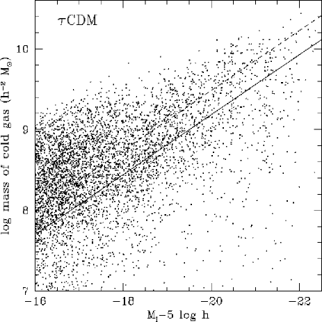
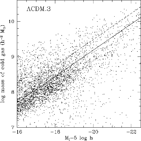
Figure 32: Small dots show the cold gas masses of the model galaxies from mock catalogs extracted from the New/Santa Cruz (fiducial) $\tau$CDM (top) and $\Lambda$CDM.3 (bottom) models. The solid line is an approximate fit to ${\rm H_{I}}$ observations [de Blok et al. (1996)]. The dashed line is the same fit, with the gas masses multiplied by a factor of two to allow for a contribution from cold gas not in the form of $H_{\rm I}$.

It should be kept in mind that this comparison rests on the assignment of model galaxy circular velocities as well as luminosities, and on the conversion from circular velocity to linewidth. In the current models we have assumed that all galaxies have perfectly flat rotation curves out to the virial radius of the halo; i.e., that the circular velocity measured by TF observations (typically at about two optical disk scale lengths) is the same as the virial velocity of the dark matter halo. This assumption clearly must break down in halos with circular velocities larger than about 350-400 km s^-1, as no known galaxies have rotation velocities this large. As we noted in Section 3, if the profiles of dark matter halos resemble the NFW profile, then $V_{c}$ at a few scale lengths will be larger than at $r_{\rm vir}$ for smaller (galaxy) mass halos, and smaller than at $r_{\rm vir}$ for larger (cluster) mass halos. In addition, the dissipative infall of baryons will modify the inner rotation curve [Blumenthal et al. (1986), Flores et al. (1993)]. Before attempting a rigorous evaluation of the Tully-Fisher relation predicted by the models, the halo and disk profiles should be modelled in more detail. We intend to address this problem in future work.

Figure 34: The $H_{\rm I}$ mass function. The two smooth lines show the Schechter function fit to the results from ?), where the lower (bold) line is the actual fit and the upper line shows the effect of increasing all the gas masses by a factor of two to account for cold gas not in the form of $\rm H_{I}$. The survey is sensitive in the range $10^{7}$ to $10^{10}\mbox{$M_{\odot}$}$, and the dashed lines show the extrapolation of the Schechter function into the unprobed region. The thin bold lines show the uncertainty in the faint end slope as given by ?). The arrows show upper limits from a complementary Arecibo survey, also mentioned in ?). The histograms show the results from the models. The top panel shows the Classic/SCDM models with different sf/fb packages, and the bottom panel shows the New/Santa Cruz (fiducial) models for different cosmologies.

5.3 Cold Gas

We now investigate the cold gas masses of galaxies in our models. This is an important counterpart to studying the luminosities of galaxies. Fig. 32 shows the mass of cold gas in the model galaxies as a function of I magnitude for two examples of our fiducial models ($\tau$CDM and $\Lambda$CDM.3). The solid line shows an approximate fit to local ${\rm H_{I}}$ data (see Fig. 12 of [de Blok et al. (1996)]). Recall that we set the free parameters to match the zero-point of this relation at $M_{I}-5\log h\sim-21.8$, assuming that the mass of “cold gas” in our model reference galaxy is approximately a factor of two larger than the observed ${\rm H_{I}}$ mass to allow for molecular hydrogen (we neglect the additional contribution of helium and ionized hydrogen). This corresponds to the typical contribution of molecular hydrogen in an Sb-Sc type galaxy [Young & Knezek (1989)]. The observations show a large scatter, comparable to the scatter in the models. The models results are consistent with the observed trend of gas mass with magnitude and the scatter in this relation. It should be noted that we have not made any morphological cuts on the model galaxies, whereas the observations are for late-type galaxies. The results look similar for all the models.

We also investigate the ${\rm H_{I}}$ mass function, or the number density of galaxies with a given ${\rm H_{I}}$ mass. This has been estimated by the survey of ?), and more recently in the blind ${\rm H_{I}}$ survey described in ?). The latter should place strong upper limits on the number of low surface brightness galaxies (unless there is a very gas poor population) because it is not optically selected. In Fig. 34 we show the $H_{\rm I}$ mass function for all the models, along with observations from ?). All of the SCDM models show a considerable excess especially on the small-mass end. The $\tau$CDM models show a somewhat smaller excess, and the other models are in good agreement with the observational limits across the range of ${\rm H_{I}}$ gas masses probed by the observations.

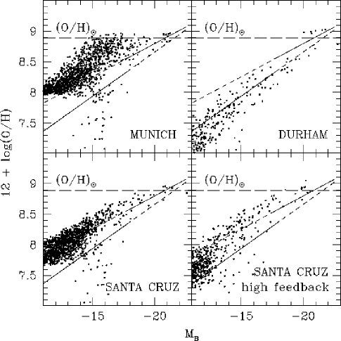
Figure 36: The metallicity-luminosity relation in the Classic/SCDM models (small dots), for galaxies within a “local group” (${V_{c}=220\>\mbox{km s${}^{-1}$}}$) sized halo. Bold lines show fits to the observed relation for bright spirals and for local dwarf galaxies (from the compilation in [Kobulnicky & Zaritsky (1998)]).

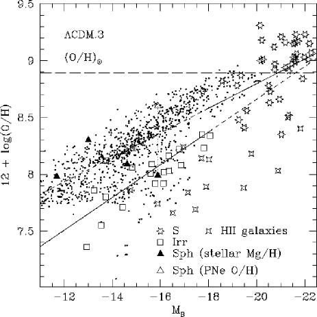
Figure 38: The metallicity-luminosity relation for a volume limited mock catalog extracted from the New/Santa Cruz (fiducial) $\Lambda$CDM.3 models. Large symbols show observations of bright spirals, dwarf irregulars and spheroidals, and HII galaxies [Kobulnicky & Zaritsky (1998)].

5.4 Metallicity-Luminosity Relation

Nearby galaxies are known to exhibit a trend between their B-band luminosities and their metal contents, in the sense that more luminous galaxies are more metal-rich. The slope of the observed relation derived for bright spirals ($M_{B}-5\log h_{50}\mathrel{\hbox{\hbox to0.0pt{\hbox{\lower 4.0pt\hbox{$\sim$}}\hss}\hbox{$<$}}}-18$) is shallower than that for nearby dwarf galaxies [Skillman et al. (1989), Richer & McCall (1995), Zaritsky et al. (1994), Kobulnicky & Zaritsky (1998)].

Although we obtain a similar trend in the models (see Fig. 36), the detailed behaviour of the observations is not well reproduced in any of the models. Recall that we have set our yield parameter $y$ in order to obtain solar metallicity in our approximately “Milky Way” sized reference galaxy. The relation that we obtain depends on the treatment of metal and gas ejection by supernovae. In the Munich package, none of the metal or gas is ejected from the halo, and this package produces a very shallow relation with a break at about $M_{B}=-15$. In the Durham package, all of the reheated gas and metals are ejected from the halo, resulting in a very steep relation even for the bright galaxies. In the Santa Cruz package, the ejection of gas and metals is modelled using the disk-halo approach. This leads to a relation which is consistent with the bright galaxies, but dwarf galaxies that are too metal-rich compared to the observations. This is the case even in the high feedback package. The Durham package produces the best agreement with the observed relation. However, it also produced an unacceptable degree of curvature on the faint end of the Tully-Fisher relation.

Figure 40: B-V colour histogram for galaxies in the New/Santa Cruz (fiducial) models, in the $\tau$CDM (top panel) and $\Lambda$CDM.3 (bottom panel) cosmologies. The shaded histogram shows the observed colour distribution of bright galaxies ($M_{B}-5\log h\geq-19.0$) from the RC3 catalog [De Vaucouleurs et al. (1991)]. The unshaded histograms show the model galaxies, selected to be brighter than $M_{B}-5\log h=-19.0$ (solid) or $M_{B}-5\log h\geq-15.5$ (dashed). Within each panel, the top half-panel shows the model results without the correction for dust reddening, and the bottom half-panel shows the results with the correction for dust.

The failure of all models in which ejected metals follow the ejected gas may indicate that metal ejection is more efficient than gas ejection. This has been proposed on the basis of high-resolution hydrodynamic simulations of dwarf galaxies [Mac Low & Ferrara (1998)]. Our results support the strongly differential ejection efficiency proposed by ?) on the basis of observations. One should use caution in interpreting the observations, however, because of possible systematic errors in the observational determination of metal abundances in different types of galaxies and using different methods [Kobulnicky et al. (1999)]. Interpreting the observations is also complicated by the presence of metallicity gradients in large galaxies, and the strong correlation of metallicity with surface brightness [Garnett (1997)]. We postpone a more careful investigation of these issues to future papers.

5.5 Colours

A familiar property of observed galaxies is the “colour-magnitude” relation: bright galaxies are observed to be redder than fainter ones. It is an often repeated statement that hierarchical models of galaxy formation generically predict that more massive objects form “later” than smaller mass objects. This statement is often misinterpreted to imply that larger mass objects should be “younger” and therefore bluer than smaller ones. If the formation time of an object is defined as the time when a given fraction of its mass has been assembled into a single progenitor, then it is true that larger mass objects have later formation times than smaller mass objects. However, if we define “age” as the time spent in the sort of environment where we expect that star formation is able to occur (i.e., within a collapsed halo), then the mean age of the material in large mass halos is older than in smaller mass halos. This is because large mass halos are associated with higher peaks in the density field, which collapse earlier.

In the SAMs, we find that when the effects of dust and metallicity are neglected, we obtain flat colour-magnitude relations or (depending on the model and the colour bands in question) bright galaxies that are only slightly redder (see Fig. 40; top panel) than the faint population. The bright galaxies are also a bit too blue overall compared with observations (the observed colour distribution of bright galaxies in the RC3 catalog [De Vaucouleurs et al. (1991)] is shown for comparison). Inclusion of dust extinction shifts the colour distribution towards the red, and shifts the bright galaxies more than the faint ones because of the differential nature of our dust recipe. This brings the optical colours into fairly good agreement with the observations. In addition, ?) have shown that the inclusion of metallicity effects on the model spectra (here we have used only the solar metallicity stellar population models) can also produce the observed colour-magnitude slope. Presumably the observed trend is a combination of these two effects.

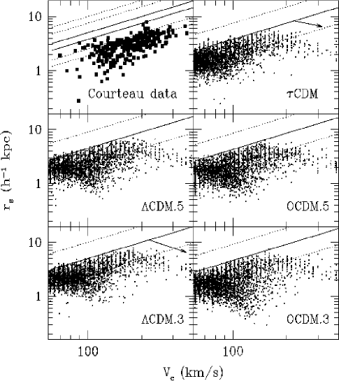
Figure 42: Exponential scale radius vs. circular velocity. The large filled squares (top left panel) show the observations of ?). The small dots show the results of the fiducial Santa Cruz models in various cosmologies as indicated. Bold solid lines show the relation we would obtain if all gas fell in from the virial radius of the halo, for $\lambda_{H}=0.05$ (50 percent point). Bold dashed lines show the same relation for $\lambda_{H}=0.025$ (10 percent) and $\lambda_{H}=0.1$ (90 percent). These vary slightly depending on cosmology. The $\tau$CDM (lower) and $\Lambda$CDM.3 (upper) relations are shown on the upper left panel with the observations as a reference point (other models are intermediate). The arrows on the $\tau$CDM and $\Lambda$CDM.3 panels show the corrections to this relation predicted from the fitting formulae of ?) (see text).

5.6 Sizes

We estimate the exponential scale radii of our model disks using the approach described in Section 2.4. We show the relationship between scale radius and circular velocity in Fig. 42. The upper left-most panel shows the observations of ?) for late-type galaxies, where $V_{c}$ is the disk rotation velocity at 2.2 scale-lengths, and $r_{s}$ is the exponential scale length in the $r$ band. In the models, the scale radius that we estimate represents the total baryonic mass (stars and cold gas) in the disk. The scale radius of the stellar mass may be smaller if star formation is more efficient in the inner parts of the disk, and the scale of the optical light may be smaller yet. The bold solid lines indicate the relation $r_{s}=1/\sqrt{2}\lambda_{H}r_{\rm vir}$, which we would obtain if the gas fell in from the virial radius of the halo. As we have discussed in Section 2.4, we have used a constant value of $\lambda_{H}=0.05$ for all halos, so the only source of scatter in the relation that we obtain is from the different cooling radii of the halos, which occur as a result of the scatter in halo merging histories (see Figure 4). The SAM dots always lie at smaller $r_{s}$ than the bold lines because the cooling radius is always smaller than the virial radius. The bold dashed lines show the same relation for $\lambda_{H}=0.1$ and $\lambda_{H}=0.025$, which are the 10 and 90 percent points of the distribution of $\lambda_{H}$ used by ?).

As we discussed in Section 2.4, we have not included the “back reaction” of baryons on the dark matter during their collapse, which will tend to lead to smaller scale radii [Blumenthal et al. (1986), Flores et al. (1993), Mo et al. (1998)] and will also modify the rotation curve. The use of a more realistic halo profile (e.g. NFW) will also change these results. The correction due to these effects, as predicted by the fitting formulae of ?), is shown by the arrows in the $\tau$CDM and $\Lambda$CDM.3 panels (the correction is relatively insensitive to cosmology, and is similar for the other models). The direction of the correction is to produce galaxies with larger $V_{\rm max}$ and smaller scale radii. The details of these corrections depend on the assumed halo profile and disk baryon fraction as well as other parameters. We intend to incorporate improved modelling of disk sizes and rotation curves into our models and present more detailed predictions of these quantities in the near future.

In the meantime, several things are worth noting. An obvious difference in the current model predictions is the break in the $r_{s}$-$V_{c}$ relation at about 200 km s^-1: the trend reverses and the scale radii start to decrease at larger $V_{c}$. This is caused by the decreasing cooling radius in halos with higher virial temperature (see Fig. 4). No such break is evident in the observations, although the sample contains a relatively small number of galaxies with $V_{c}>200$ km s^-1. The rightward shift indicated by the arrows (due to “peaking up” of the rotation curve caused by the effects mentioned above) may solve this problem, but will also make the disks too small at a given $V_{c}$ compared to the Courteau data. Most of the effects we have mentioned indicate that we may already be systematically over-estimating the disk sizes. We therefore may be facing a puzzle similar to the “angular momentum” problem found in N-body simulations with hydrodynamics (i.e., disks are too small and concentrated at a given circular velocity compared to observations, cf. [Steinmetz & Navarro (1999)]).

6 Summary and Discussion

We have presented new semi-analytic models of galaxy formation and shown that these models can reproduce many key observational properties of galaxies in the local Universe. Our approach is similar to that introduced by ?) and ?), but we have introduced several modified or new ingredients, including:

• Somerville-Kolatt method for “planting” merger trees ([Somerville & Kolatt (1998)]; shown to give good agreement with merger trees extracted from N-body simulations in [Somerville et al. (1998)]).

• Improved Sheth-Tormen model [Sheth & Tormen (1999)] for the mass function of dark matter halos (an improved version of the Press-Schechter model which gives much better agreement with the reusults of N-body simulations).

• “Dynamic halo” model for gas cooling (includes the effects of halo merger events on the density and temperature of the hot halo gas).

• “Disk-halo” model for supernovae feedback (models the ejection of cold gas from the disk and global (dark matter) potential seperately)

• Dust extinction based on the empirical recipe of ?)

• Galaxy mergers due to satellite collisions, using the simulation-based approximation of ?)

• More detail modelling of starbursts based on hydrodynamical simulations [Mihos & Hernquist (1994), Mihos & Hernquist (1996)]

We have investigated several different “packages” of recipes for star formation and supernovae feedback in order to gain better understanding of the importance of the way in which these processes are parameterized. We have also illustrated the results of varying the most important free parameters in our models.

We have addressed the long-standing problem of the physical explanation of the observed luminosity function within CDM-type hierarchial models of structure formation. Early in the history of CDM, it was noted that the mass function of dark matter halos, whether predicted by analytic models like Press-Schechter or derived from N-body simulations, has a steep power-law slope ($\alpha\sim-2$) for masses $\mathrel{\hbox{\hbox to0.0pt{\hbox{\lower 4.0pt\hbox{$\sim$}}\hss}\hbox{$<$}}}10^{14}\mbox{$h^{-1}$ $M_{\odot}$}$, and an exponential cut-off at $\sim 10^{14}\mbox{$h^{-1}$ $M_{\odot}$}$, much larger than the expected mass of the halos surrounding $L_{*}$ galaxies, as estimated from their internal velocity dispersions. It was proposed that feedback due to supernovae could suppress star formation in small mass halos, leading to a flatter faint end slope, and inefficient gas cooling in large mass halos could cause the “knee” at $L_{*}$. However, the first generation of SAMs, which attempted to actually model these processes in some detail, encountered some difficulties. The Munich models produced the correct (B-band) TFR slope, but the faint-end slope of the luminosity function was still too steep. In addition, unless an ad-hoc cutoff was applied, in which gas cooling was turned off by hand in halos larger than 500 km s^-1, these models did not produce a “knee” in the luminosity function and showed an excess of very bright galaxies. These models were normalized to the observed luminosity of the Milky Way Galaxy, and were claimed to reproduce the observed zeropoint of the local B-band TFR. The Durham models produced a luminosity function with a “knee”, and the free parameters were adjusted in order to match its location with that of the observed B-band luminosity function. Their luminosity functions showed a flatter faint-end slope, in better agreement with observations, but produced a TFR with a zeropoint offset of about 2 magnitudes and a serious deviation from the observed power-law behavior on the small $V_{c}$ end.

We have clarified the reasons for some of these differences. First, we have explained how it is that, although the Munich group claimed to reproduce the observed zeropoint of the TFR, in fact their model galaxies were $\sim 2$ magnitudes too faint at a given circular velocity compared to the TFR derived from recent large I-band samples. Using our models with sf/fb recipes chosen to be similar to those of the Munich and Durham group, we showed that when the models are normalized in the same way, the luminosity function and TFR are nearly identical for bright/large $V_{c}$ galaxies ($M_{B}-5\log h\mathrel{\hbox{\hbox to0.0pt{\hbox{\lower 4.0pt\hbox{$\sim$}}\hss}\hbox{$<$}}}-20$, $V_{c}\mathrel{\hbox{\hbox to0.0pt{\hbox{\lower 4.0pt\hbox{$\sim$}}\hss}\hbox{$>$}}}220$ km s^-1). The results differ substantially only for faint/small $V_{c}$ galaxies, and this difference can be traced mainly to the stronger supernovae feedback recipe assumed by the Durham group. We demonstrate this by showing that as we turn up the parameter that represents the fraction of supernovae energy deposited in the cold gas ($\epsilon_{SN}^{0}$), our results move continuously from a situation resembling the Munich models (steep LF, powerlaw TFR) to one resembling the Durham models (flat LF, curved TFR). This works because in our “disk-halo” feedback model, the parameter $\epsilon_{SN}^{0}$ affects not only the total amount of gas that is reheated, but also the fraction that is ejected from the halo. We issue a warning, however, that although the supernovae feedback efficiency is the dominant factor determining these results at $z=0$, the redshift evolution is also very sensitive to the assumed star formation recipe. This will be illustrated in detail in a companion paper [Somerville et al. (1999)].

Figure 44: The effect of various model variations on the model B and K-band luminosity functions, introduced one by one. The new feature of each model is in italics. Model 1: Munich-style feedback, original Press-Schechter mass function, static halo cooling, SCDM, no dust correction. Model 2: disk-halo feedback, original Press-Schechter mass function, static halo cooling, SCDM, no dust correction. Model 3: disk-halo feedback, Sheth-Tormen mass function, static halo cooling, SCDM, no dust correction. Model 4: disk-halo feedback, Sheth-Tormen mass function, dynamic halo cooling, SCDM, no dust correction. Model 5: disk-halo feedback, Sheth-Tormen mass function, dynamic halo cooling, $\Lambda$CDM.5, no dust correction. Fiducial model: disk-halo feedback, Sheth-Tormen mass function, dynamic halo cooling, $\Lambda$CDM.5, with dust correction. In the top panel, the bold lines show the observed B-band luminosity function from the 2dF survey (higher line) and the APM survey (lower line). In the bottom panel, the bold lines show the observed K-band luminosity function from ?) and ?).

We have shown that the observed B and K band luminosity functions and the Tully-Fisher relation can be reproduced simultaneously in our models. This improvement is not due to any one effect but is the result of many combined factors, as summarized below. We first normalize our models to fix the zeropoint of the TFR for a typical $L_{*}$ galaxy. This requires us to use a stellar mass-to-light ratio approximately a factor 2 to 3 times higher than the published Munich and Durham models, but corresponds to taking the predictions of the Bruzual-Charlot stellar population models at close to face value and is in better agreement with observational estimates. If we then use cooling, feedback, and star formation recipes similar to the published Munich models, we obtain a B-band luminosity function with several problems: the overall normalization is too high, the faint end slope is too steep, and there is a “tail” of bright galaxies (see Fig. 44, model 1). Fig. 44 shows the effect of introducing various changes, one by one, which eventually lead to our fiducial model choices. These are summarized below. We remark whether the effect is important on the bright ($M_{B}-5\log h\sim-21.5$) or faint ($M_{B}-5\log h\sim-16.5$) end of the luminosity function, and by what factor the B-band luminosity function changes at this magnitude. These factors should be considered approximate only, and may be read from the top panel of Fig. 44.

• “disk-halo” feedback model (faint end, factor of 2.5)

• Sheth-Tormen mass function (overall, factor of 1.5)

• “dynamic halo” cooling model (bright end, factor of 3)

• low $\Omega\sim 0.5$ cosmology (bright end, factor of 1.6; faint end, factor of 3)

• dust extinction (bright end, factor of 16)

Note that the observations have also changed — the solid bold curve in Fig. 44 shows the luminosity function derived from the recent 2dF survey [Folkes et al. (1999)], which is in excellent agreement with the LF from the deep ESO slice [Zucca et al. (1997)]. Both have considerably steeper faint-end slopes than the LF derived from the APM survey ?), which was the standard at the time of much of the earlier modelling. The more recent observations are easier to reconcile with the models. A similar accounting may be done for the K-band luminosity function (Fig. 44, bottom panel).

We therefore conclude that the very strong feedback and suppression of star formation in small $V_{c}$ galaxies assumed in the Durham models is not necessary in order to reproduce the observed luminosity function, and is disfavored as it produces curvature on the small $V_{c}$ end of the TFR.

In our $\Omega_{0}=1$ models (SCDM and $\tau$CDM), we find that in order to produce galaxies with large enough luminosities and gas masses, we must assume values of the baryon fraction ($f_{\rm baryon}\sim 0.1-0.12$) which are rather high compared with estimates from observations of high-redshift deuterium [Tytler et al. (1999)], though consistent with estimated baryon fractions in groups and clusters. In our best $\Omega_{0}=1$ models, we find good agreement with the general shape of the LF, but the model LF is too high by an overall factor of $\sim 3$ in B and 2.5 in K. The mass function of cold gas is also a factor of $\sim 5$ higher than estimates from blind ${\rm H_{I}}$ surveys. In order to reconcile these models with observations, we would have to believe that there is a substantial population of galaxies, including some with large total masses, that are undetected in optical emission or radio emission from cold ${\rm H_{I}}$ gas. This seems unlikely, though not impossible. Thus, although we cannot say that $\Omega_{0}=1$ is ruled out, our results are certainly more easily compatible with models in which $\Omega_{0}\sim 0.3-0.5$, with or without a cosmological constant.

The same fiducial models produce good agreement with observations of the mass function of cold ${\rm H_{I}}$ gas and the magnitude-${\rm H_{I}}$-mass relation. When we normalize our models to produce a “Milky-Way” galaxy with solar metallicity, the metallicities of dwarf galaxies in our models are somewhat higher than the average metallicity of nearby dwarf galaxies, i.e. the slope of the metallicity-luminosity relation is too shallow. This may be evidence that metals are ejected by supernovae more efficiently than the cold gas, or an indication that our “constant yield” approach to modelling chemical evolution is too simplistic. Alternatively, it may be due to systematic uncertainties in deriving observational estimates of metal abundances in different types of galaxies [Kobulnicky et al. (1999)]. Our fiducial models produce good qualitative agreement with the optical colors of bright galaxies, and reproduce the observed color-magnitude trend, when dust extinction is included. Although the relationship between the exponential scale radius and circular velocity of disks that we estimate is in reasonably good qualitative agreement with observations, we conclude that more detailed modelling is necessary.

A great strength of the SAM technique is that one can make self-consistent predictions pertaining to a wide variety of observations. In companion papers, we investigate our predictions for the properties of high-redshift galaxies and the history of stars, cold gas, and metals at high redshift [Somerville et al. (1999)], and extend our predictions for local galaxies to shorter (far UV) and longer (far IR to sub-mm) wavelengths [Somerville et al. (1999), Bullock et al. (1999)].

A Spherical Collapse in a General Cosmology

Figure A2: The relationship between halo mass and virial velocity from the spherical tophat model, at $z=0$ (bottom set of lines), $z=1$, and $z=3$ (top), for the cosmologies discussed in the text. The relation depends (weakly) on cosmology and (strongly) on redshift.

We need to be able to relate the mass, radius, and velocity dispersion of dark matter halos for any given redshift. This is made possible using the spherical collapse model, one of the apparently gross oversimplifications that seems to work surprisingly well. We imagine a spherical patch of the universe with a uniform overdensity $\delta_{i}$ within a radius $r_{i}$ at a very early time $t_{i}$ (often called a “top-hat” perturbation). We assume that the collapsing shells of matter do not cross. If we consider a particle at radius $r$, Birkhoff’s theorem [Birkhoff (1923)] tells us that we can ignore the mass outside this radius in computing the motion of the particle. The equation of motion for our particle (in physical, rather than comoving, coordinates) is then

$$\frac{d^{2}r}{dt^{2}}=-\frac{GM}{r^{2}}+\frac{\Lambda}{3}r$$ (A1)

where $M=(4\pi/3)r_{i}^{3}\rho_{b}(t_{i})(1+\delta_{i})$ and $\rho_{b}(t_{i})$ is the background density of the universe at $t_{i}$. Integrating this equation gives

$$\dot{r}=H_{0}\left[\frac{\Omega_{0}}{r}(1+\delta_{i})\frac{r_{i}^{3}}{a_{i}^{3}}+\Omega_{\Lambda}r^{2}-K\right]$$ (A2)

where $K$ is a constant of integration. We may fix this by noting that if we have picked $t_{i}$ early enough that $\Omega\sim 1$ at that time, linear theory tells us that the initial velocity is

$$\dot{r}(t_{i})=H_{0}r_{i}\left(1-\frac{\delta_{i}}{3}\right)\sqrt{\frac{\Omega_{0}}{a_{i}^{3}}+\frac{\Omega_{R}}{a_{i}^{2}}+\Omega_{\Lambda}}.$$ (A3)

[Peebles (1984)]. At the point of maximum expansion, or “turnaround”, $\dot{r}=0$. If we set equation (A3) to zero, we obtain a cubic equation for $r_{ta}$, the radius of the perturbation at turnaround, which must be solved numerically for the general cosmology given here, but for special cases it can be solved analytically (cf. [Padmanabhan (1993)]). From a symmetry argument, we note that the time when the perturbation collapses to a point, $t_{\rm coll}$, is always twice $t_{ta}$ (the time at maximum expansion). We can now write an implicit equation for the mass of a perturbation that is collapsing at $t_{\rm coll}$:

$$t_{\rm coll}=2\int_{0}^{r_{ta}}\frac{dr}{\dot{r}}\,.$$ (A4)

We know the mass and the radius at turnaround, so we can calculate the density of the perturbation at turnaround, $\rho_{ta}$.

Of course the perturbation will not really collapse to a point. Before that happens, shell crossing will occur, and it will virialize. We can find the radius after viralization in terms of the turnaround radius using the virial theorem. The total energy at turnaround is [Lahav et al. (1991)]

$$E=U_{G,ta}+U_{\Lambda,ta}=-\frac{3}{5}\frac{GM^{2}}{r_{ta}}-\frac{1}{10}\Lambda Mr_{ta}^{2}$$ (A5)

where the second term is due to the cosmological constant. Now using the virial theorem for the final state:

$$T_{f}=-\frac{1}{2}U_{G,f}+U_{\Lambda,f}\,.$$ (A6)

From conservation of energy we then have $\frac{1}{2}U_{G,f}+2U_{\Lambda,f}=U_{G,ta}+U_{\Lambda,ta}$. This leads to a cubic equation for the ratio of the virial radius $r_{\rm vir}$ to the turnaround radius $r_{ta}$. We now know $r_{\rm vir}$ and can write down the virial density

$$\Delta_{c}(z)\equiv\frac{\rho_{\rm vir}\Omega(z)}{\Omega_{0}\rho_{c}^{0}(1+z)^{3}}.$$ (A7)

We now have a relationship between the mass, virial radius, and collapse redshift $z$. If we assume a radial profile for the virialized halo, we can use the virial theorem again to relate these quantities to the velocity dispersion. If we assume that the halo is a singular isothermal sphere, $\rho\propto r^{-2}$, truncated at the virial radius, then we have

$$\frac{3}{2}\sigma^{2}=\frac{GM}{2r_{\rm vir}}-\frac{\Lambda r_{\rm vir}^{2}}{18}$$ (A8)

or, in terms of the circular velocity $V_{c}$, assuming $V_{c}^{2}=2\sigma^{2}$:

$$V_{c}^{2}=\frac{GM}{r_{\rm vir}}-\frac{\Omega_{\Lambda}}{3}H_{0}^{2}r_{\rm vir}^{2}$$ (A9)

We can now translate between mass and velocity dispersion at any given redshift. Note that in universes with a non-zero cosmological constant, halos of a given circular velocity are less massive because of the $\Lambda$ contribution to the energy.

In practice, we use the fitting formula of ?) for the virial density:

$$\Delta_{c}=18\pi^{2}+82x-39x^{2}$$ (A10)

for a flat universe and

$$\Delta_{c}=18\pi^{2}+60x-32x^{2}$$ (A11)

for an open universe, where $x\equiv\Omega(z)-1$. This formula is accurate to 1% in the range $0.1\leq\Omega\leq 1$, which is more than adequate for our purposes. We now can write down the general expression for $r_{\rm vir}$ in closed form.

$$r_{\rm vir}=\left[\frac{M}{4\pi}\frac{\Omega(z)}{\Delta_{c}(z)\Omega_{0}\rho_{c,0}}\right]^{1/3}\frac{1}{1+z}.$$ (A12)

In conjunction with equation A9, this allows us to calculate the circular velocity and viral radius for a halo with a given mass at any redshift $z$. These expressions are valid for open cosmologies with $\Lambda=0$ and flat cosmologies with non-zero $\Lambda$.

References

- Barnes & Efstathiou (1987) Barnes J., Efstathiou G., 1987, ApJ, 319, 575
- Barnes & Hernquist (1992) Barnes J., Hernquist L., 1992, ARA&A, 30, 705
- Baugh et al. (1997) Baugh C., Cole S., Frenk C., Lacey C., 1997, astro-ph/9703111
- Baugh et al. (1996a) Baugh C. M., Cole S., Frenk C. S., 1996a, MNRAS, 283, 1361
- Baugh et al. (1996b) Baugh C. M., Cole S., Frenk C. S., 1996b, MNRAS, 282L, 27
- Bernstein et al. (1994) Bernstein G. et al., 1994, AJ, 101, 1231
- Binney & Tremaine (1987) Binney J., Tremaine S., 1987, Galactic Dynamics. Princeton Univ. Press, Princeton, NJ
- Birkhoff (1923) Birkhoff G., 1923, Relativity and Modern Physics. Harvard University Press, Cambridge
- Blumenthal et al. (1986) Blumenthal G., Faber S., Flores R., Primack J., 1986, ApJ, 301, 27
- Blumenthal et al. (1984) Blumenthal G., Faber S., Primack J., Rees M., 1984, Nat, 311, 517
- Bond et al. (1991) Bond J. R., Cole S., Efstathiou G., Kaiser N., 1991, ApJ, 379, 440
- Bower (1991) Bower R., 1991, MNRAS, 248, 332
- Bruzual & Charlot (1993) Bruzual A., Charlot S., 1993, ApJ, 405, 538
- Bryan & Norman (1997) Bryan G., Norman M., 1997, ApJ, in press, astro-ph/9710107
- Bullock et al. (1999) Bullock J., Somerville R., Primack J., 1999, in preparation
- Bunn & White (1997) Bunn E. F., White M., 1997, ApJ, 480, 6
- Cardelli et al. (1989) Cardelli J., Clayton G., Mathis J., 1989, ApJ, 345, 245
- Charlot et al. (1996) Charlot S., Worthey G., Bressan A., 1996, ApJ, 457, 625
- Cole (1991) Cole S., 1991, ApJ, 367, 45
- Cole et al. (1994) Cole S., Aragón-Salamanca A., Frenk C., Navarro J., Zepf S., 1994, MNRAS, 271, 781
- Copi et al. (1996) Copi C., Schramm D., Turner M., 1996, Nucl. Phys. B., S51B, 66
- Courteau (1996) Courteau S., 1996, ApJS, 103, 363
- da Costa et al. (1994) da Costa L. et al., 1994, ApJ, 424, L1
- Dalcanton et al. (1997) Dalcanton J., Spergel D., Gunn J., Schneider D., Schmidt M., 1997, preprint
- Dalcanton et al. (1997) Dalcanton J., Spergel D., Summers F., 1997, ApJ, 482, 659
- de Blok et al. (1996) de Blok W., McGaugh S., van der Hulst J., 1996, MNRAS, 283, 18
- De Vaucouleurs et al. (1991) De Vaucouleurs G., De Vaucouleurs A., Corwin H., Buta R., Paturel G., Fouque P., 1991, Third Reference Catalogue of Bright Galaxies. Springer-Verlag
- Dekel & Silk (1986) Dekel A., Silk J., 1986, ApJ, 303, 39
- Efstathiou et al. (1992) Efstathiou G., Bond J., White S., 1992, MNRAS, 258, 1
- Evrard et al. (1996) Evrard A., Metzler C., Navarro J., 1996, ApJ, 469, 494
- Fall & Efstathiou (1980) Fall S., Efstathiou G., 1980, MNRAS, 193, 189
- Flores et al. (1993) Flores R., Primack J., Blumenthal G., Faber S., 1993, ApJ, 412, 443
- Folkes et al. (1999) Folkes S. et al., 1999, MNRAS, accepted (astro-ph/9903456)
- Forcado-Miro (1997) Forcado-Miro M., 1997, astro-ph/9712205
- Gardner et al. (1997) Gardner J., Sharples R., Frenk C., Carrasco B., 1997, ApJ, 480, 99
- Garnett (1997) Garnett D., 1997, in Friedli D., Edmunds M., Robert C., Drissen L., ed, Abundance Profiles: Diagnostic Tools for Galaxy History. ”ASP Conf. Ser. Vol. 147, p. 78”
- Gilmore (1997) Gilmore G., 1997, in International Dark Matter 96. World Scientific, astro-ph/9702081
- Giovanelli et al. (1997) Giovanelli R., Haynes M., Da Costa L., Freudling W., Salzer J., Wegner G., 1997, ApJ, 477, L1
- Górski et al. (1996) Górski K. M., Banday A. J., Bennett C. L., Hinshaw G., Kogut A., Smoot G. F., Wright E. L., 1996, ApJ, 464, L11
- Gross (1997) Gross M., 1997, Ph.D. thesis, University of California, Santa Cruz, http://fozzie.gsfc.nasa.gov
- Gross et al. (1998) Gross M. A. K., Somerville R. S., Primack J. R., Holtzman J., Klypin A. A., 1998, MNRAS, submitted, astro-ph/9712142
- Guiderdoni & Rocca-Volmerange (1987) Guiderdoni B., Rocca-Volmerange B., 1987, A&A, 186, 1
- Heyl et al. (1995) Heyl J. S., Cole S., Frenk C., Navarro J., 1995, MNRAS, 274, 755
- Hu & Sugiyama (1996) Hu W., Sugiyama N., 1996, ApJ, 471, 542
- Kauffmann (1995) Kauffmann G., 1995, MNRAS, 274, 153
- Kauffmann (1996a) Kauffmann G., 1996a, MNRAS, 281, 487
- Kauffmann (1996b) Kauffmann G., 1996b, MNRAS, 281, 475
- Kauffmann & Charlot (1996) Kauffmann G., Charlot S., 1996, MNRAS, 294, 705
- Kauffmann et al. (1994) Kauffmann G., Guiderdoni B., White S. D. M., 1994, MNRAS, 267, 981
- Kauffmann et al. (1997) Kauffmann G., Nusser A., Steinmetz M., 1997, MNRAS, 286, 795
- Kauffmann & White (1993) Kauffmann G., White S., 1993, MNRAS, 261, 921
- Kauffmann et al. (1993) Kauffmann G., White S., Guiderdoni B., 1993, MNRAS, 264, 201
- Kobulnicky et al. (1999) Kobulnicky H., Kennicutt R., Pizagno J., 1999, ApJ, in press (astro-ph/9811006)
- Kobulnicky & Zaritsky (1998) Kobulnicky H., Zaritsky D., 1998, ApJ, in press (astro-ph/9808081)
- Kravtsov et al. (1998) Kravtsov A., Klypin A., Bullock J., Primack J., 1998, ApJ, in press, astro-ph/9708176
- Lacey & Cole (1993) Lacey C., Cole S., 1993, MNRAS, 262, 627
- Lacey et al. (1993) Lacey C., Guiderdoni B., Rocca-Volmerange B., Silk J., 1993, ApJ, 402, 15
- Lacey & Silk (1991) Lacey C., Silk J., 1991, ApJ, 381, 14
- Lahav et al. (1991) Lahav O., Lilje P. B., Primack J. R., Rees M. J., 1991, MNRAS, 251, 128
- Lemson & Kauffman (1997) Lemson G., Kauffman G., 1997, MNRAS, submitted, astro-ph/9710125
- Loveday (1996) Loveday J., 1996, MNRAS, 278, 1025
- Loveday et al. (1992) Loveday J., Peterson B., Efstathiou G., Maddox S., 1992, ApJ, 390, 338
- Mac Low & Ferrara (1998) Mac Low M.-M., Ferrara A., 1998, ApJ, in press (astro-ph/9801237)
- Makino & Hut (1997) Makino J., Hut P., 1997, ApJ, 481, 83
- Martin (1998) Martin C., 1998, ApJ (in press) (astro-ph/9810233)
- Marzke et al. (1994) Marzke R., Huchra J., Geller M., 1994, ApJ, 428, 43
- Mihos & Hernquist (1994) Mihos J., Hernquist L., 1994, ApJ, 425, 13
- Mihos & Hernquist (1996) Mihos J., Hernquist L., 1996, ApJ, 464, 641
- Mo et al. (1998) Mo H., Mao S., White S., 1998, MNRAS, 295, 319
- Mohr et al. (1999) Mohr J., Mathiesen B., Evrard A., 1999, ApJ, in press (astro-ph/9901281)
- Mushotzky & Loewenstein (1997) Mushotzky R., Loewenstein M., 1997, ApJ, 481, 63
- Navarro et al. (1995) Navarro J., Frenk C., White S., 1995, MNRAS, 275, 56
- Navarro et al. (1996) Navarro J. F., Frenk C. S., White S. D. M., 1996, ApJ, 462, 563
- Padmanabhan (1993) Padmanabhan T., 1993, Structure Formation in the Universe. Cambridge Univ. Press, New York
- Peebles (1984) Peebles P., 1984, ApJ, 284, 439
- Pierce & Tully (1988) Pierce M., Tully B., 1988, ApJ, 330, 579
- Pierce & Tully (1992) Pierce M., Tully B., 1992, ApJ, 387, 47
- Primack et al. (1995) Primack J. R., Holtzman J., Klypin A., Caldwell D. O., 1995, Phys. Rev. Lett., 74, 2160
- Rao & Briggs (1993) Rao S., Briggs F., 1993, ApJ, 419, 515
- Ratcliffe et al. (1997) Ratcliffe A., Shanks T., Parker Q., Fong R., 1997, astro-ph/9702216
- Richer & McCall (1995) Richer M., McCall M., 1995, ApJ, 445, 642
- Scalo (1986) Scalo J., 1986, Fundam. Cosmic Phys., 11, 1
- Shanks et al. (1984) Shanks T., Stevenson P., Fong R., MacGillivray H., 1984, MNRAS, 206, 767
- Sheth & Tormen (1999) Sheth R., Tormen G., 1999, MNRAS, submitted (astro-ph/9901122)
- Simien & de Vaucouleurs (1986) Simien F., de Vaucouleurs G., 1986, ApJ, 302, 564
- Skillman et al. (1989) Skillman E., Kennicutt R., Hodge P., 1989, ApJ, 347, 875
- Somerville (1997) Somerville R., 1997, Ph.D. thesis, University of California, Santa Cruz, http://www.fiz.huji.ac.il/ rachels/thesis.html
- Somerville et al. (1999) Somerville R., Bullock J., MacMinn D., Primack J., 1999 (in preparation)
- Somerville & Kolatt (1998) Somerville R., Kolatt T., 1998, MNRAS, in press, astro-ph/9711080
- Somerville et al. (1998) Somerville R., Lemson G., Kolatt T., Dekel A., 1998, MNRAS, submitted, astro-ph/9807277
- Somerville et al. (1999) Somerville R., Primack J., Faber S., 1999, MNRAS, submitted, astro-ph/9806228
- Steinmetz (1997) Steinmetz M., 1997, in Bonometto S., Primack J., Provenzale A., ed, Dark Matter in the Universe. IOS Press
- Steinmetz & Navarro (1999) Steinmetz M., Navarro J., 1999, ApJ, 513, 555
- Sutherland & Dopita (1993) Sutherland R., Dopita M., 1993, ApJS, 88, 253
- Szokoly et al. (1998) Szokoly G., Subbarao M., Connolly A., Mobasher B., 1998, ApJ, 492, 452
- Tormen (1998) Tormen G., 1998, MNRAS, in press, astro-ph/9802290
- Tozzi & Governato (1997) Tozzi P., Governato F., 1997, in S. D’Odorico A. F., Giallongo E., ed, The Young Universe. A.S.P. Conf. Ser.
- Tully & Fouqué (1985) Tully R., Fouqué P., 1985, ApJS, 58, 67
- Tully et al. (1997) Tully R. et al., 1997, preprint
- Tytler et al. (1999) Tytler D., Burles S., Lu L., Fan X.-M., Wolfe A., Savage B., 1999, ApJ, in press (astro-ph/9810217)
- Wang & Heckman (1996) Wang B., Heckman T., 1996, ApJ, 457, 645
- Weinberg et al. (1997) Weinberg D., Hernquist L., Katz N., 1997, ApJ, 477, 8
- White & Frenk (1991) White S., Frenk C., 1991, ApJ, 379, 52
- White et al. (1993) White S., Navarro J., Evrard A., Frenk C., 1993, Nature, 366, 429
- Willick et al. (1996) Willick J., Courteau S., Faber S., Burstein D., Dekel A., Kolatt T., 1996, ApJ, 457, 460
- Willick et al. (1995) Willick J., Courteau S., Faber S., Dekel A., 1995, ApJ, 446, 12
- Young & Knezek (1989) Young J. S., Knezek P., 1989, ApJ, 347, L55
- Zaritsky et al. (1994) Zaritsky D., Kennicutt R., Huchra J., 1994, ApJ, 420, 87
- Zucca et al. (1997) Zucca E. et al., 1997, A&A, 326, 477
- Zwaan et al. (1997) Zwaan M., Briggs F., Sprayberry D., Sorar E., 1997, astro-ph/9707109