White dwarf stars and the Hubble Deep Field

1 Introduction

The value of the Hubble Deep Field to study of the remote regions of the observable Universe is difficult to overstate, as the many exciting results of this workshop are ample testament. However, an added bonus of the HDF is that, although it a very narrow angle survey, the depth of the HDF results in its sampling a significant volume of the halo of our galaxy. Thus it is useful for the purposes of detecting (or placing upper limits on the distribution of) intrinsically faint stars, such as white dwarfs. In this capacity, the HDF can say some important things about the possible constituents of the baryonic dark matter in the halo of the Milky Way, as well as constrain the physics of white dwarf formation and cooling.

Such an investigation is timely since white dwarfs could provide a significant fraction of the total mass of the halo of the Milky Way. The MACHO observations of microlensing events in the direction of the LMC suggests that up to 50% of the dark matter halo of the Milky Way could be comprised of faint Population II white dwarf stars (Alcock et al. [1997]). Thus, constraints on the population of halo white dwarfs from the HDF can directly address this possible partial explanation of the nature of the dark halo of the Milky Way.

In this review, I hope to illustrate how the HDF can be used to constrain the luminosity function of halo white dwarfs. I begin with a brief summary of the observed white dwarf luminosity function (WDLF) of the galactic disk, and show how the HDF serves as a probe of the WDLF for the halo. I then review the theoretical background used in interpreting the WDLF in terms of the theory of white dwarf evolution and cooling, and the history of star formation in the galaxy. We are then in a position to explore the theoretical WDLF, beginning with the WDLF of the disk. We then move to a theoretical examination of the WDLF of the halo population. The results of searches for white dwarfs on the HDF can then be examined in terms of the halo white dwarf population.

1.1 White dwarf stars

White dwarf stars represent the final stage of evolution of stars like our sun. They represent the ultimate fate of all stars with masses less than about 8 $M_{\odot}$, and are the natural consequence of the finite fuel supply of these stars. Upon exhaustion of their nuclear fuels of hydrogen and helium, these stars lack sufficient mass to take advantage of the limited return of carbon fusion, and are doomed to gravitational collapse. Upon reaching a radius comparable to that of the Earth, the inner cores of these stars support themselves almost entirely by electron degeneracy pressure. Their final transformation is through the gradual release of heat that has been stored within them during the prior stages of nuclear burning.

There is a simple and compelling reason to care about white dwarf stars. It can be shown that 98% of all stars are or will be white dwarfs! In terms of stellar mass, 94% of all matter in stars is either already locked-up in white dwarfs, or is in stars that will eventually become white dwarfs; a mere 6% of matter is destined to be, or already incorporated in neutron stars, and an insignificant amount is on the black hole path.

The basic theory of white dwarf stars was stimulated by their identification, early in this century, as a class of stars with observable luminosity but very small radius. The solution to this mystery, by Chandrasekhar and Fowler, neatly integrated the then–new sciences of quantum mechanics and relativity with astrophysics. Their work was essentially a complete description of the inner workings of cool white dwarf stars. While Chandrasekhar’s theory is indeed elegant, in the later half of this century we have come to recognize that these stars represent a rich storehouse of information on the evolution of all stars. This information is available through examination of the luminosity function of white dwarf stars.

The relatively recent discovery of white dwarfs is evidence that they are relatively hard to find. Almost all white dwarfs that we know of are in the immediate solar neighborhood; 50% of known white dwarfs lie within 24 parsecs of the Sun. White dwarf discoveries have come from surveys of stars with large proper motions, searches for faint blue objects, and examination of faint members of common proper motion pairs. All three produce candidate objects that require spectroscopic follow-up observations for confirmation. Spectroscopic follow-up has identified a large number of white dwarf stars. However, the selection effects involved in such surveys are thorny to account for, and make statistical studies suspect.

The most successful recent surveys for producing new white dwarf identifications have been surveys for faint but excessively blue stars. A prime example is the Palomar–Green (PG) survey (Green et al. 1986) for blue objects out of the galactic plane. While the PG survey (and others like it) are designed for discovery of quasars, they are almost optimally designed to pick out white dwarf stars. Once again, spectroscopic follow-up is required, but such surveys have an advantage in that they produce magnitude–limited samples, and therefore are without the peculiar selection effects associated with proper–motion identifications. With the success of the the PG survey, others are underway, such as the Montreal–Cambridge survey (Demers et al. [1986]) and the Edinburgh–Cape survey (Stobie et al. [1987], Kilkenny et al. [1991]).

Because of the relatively narrow range in masses of white dwarfs (and their confinement to a line of constant radius in the H–R diagram) the Greenstein colors allow a fair determination of the absolute visual magnitude $M_{v}$. In this system, the (U-V) color provides a useful indicator for the temperature of hot white dwarfs, while the (G-R) color index works best for cooler white dwarfs. Conversion of $M_{v}$ to bolometric magnitude $M_{bol}$ requires model atmosphere bolometric corrections, such as given in Greenstein ([1976]) for cool hydrogen–atmosphere white dwarfs. Of course, when parallax measurements are available, more accurate estimates of individual values of $M_{v}$ and $M_{bol}$ are possible.

1.2 The observed white dwarf luminosity function and the age of the Galactic disk

Using estimates of $M_{v}$, one can construct a luminosity function for white dwarfs. The luminosity function is a representation of the relative space densities of white dwarfs with given absolute magnitudes, usually plotted in terms of number of stars per cubic parsec per unit bolometric magnitude, versus luminosity. This luminosity function for low luminosities by Liebert et al. ([1988]) used data on stars in the Luyten ([1979]) survey. An example of the observed luminosity function is shown in Figure 1, with data from ([1988]). The luminosity function increases steadily with decreasing luminosity. As could be expected, the cooler a white dwarf is, the more slowly it cools and fades, and so the number increases with lower temperature and luminosity.

Figure 1: The luminosity function of DA white dwarfs. Data points are from Fleming et al. ([1986]) and Liebert et al. ([1988]). The line is a representative theoretical luminosity function using the pure carbon white dwarf models of Winget et al. ([1987]) and a disk age of 8 Gyr.

However, there is a steep turn–down in the luminosity function below $10^{-4.4}L_{\odot}$ that requires explanation. This turn–down is the result of the finite time that white dwarfs in the solar neighborhood, and by extension in our galaxy, have had to cool. The time it takes for white dwarfs to fade to below this luminosity must be longer than the age of the galaxy itself. Thus the luminosity of this cut–off is a direct measure of the age of our galaxy. For Figure 1, I show a sample theoretical luminosity function calculated with simple models of pure carbon white dwarfs published by Winget et al. ([1987]). Matt Wood’s results ([1992]) using the best available white dwarf models and observed luminosity functions, indicate that the age of the galactic disk in the vicinity of the Sun is $9.3\pm 1.5$ Gyr. From the shape of the luminosity function, it is apparent that the star formation rate has been roughly constant over the history of the disk. Had there been bursts of star formation at some times, these bursts would have produced bumps along the observed luminosity function that are not seen in the data (Wood [1992], Iben & Laughlan [1989]).

1.3 Other ways of finding white dwarfs: the HDF and MACHO searches

The techniques described above are adequate for studying relatively bright white dwarfs that lie reasonably close to the Sun. As such, they are targeted for white dwarfs from the disk of the galaxy. Halo white dwarfs, on the other hand, could escape detection in these surveys by several means. If they are not close to the Sun, such halo white dwarfs could easily be fainter than the magnitude limits of these surveys. With the high velocities expected for halo stars, halo white dwarfs brighter than the limiting magnitude of current surveys could have enormous proper motions; thus they would have escaped detection by having proper motions larger than the upper limit of proper motion studies.

The HDF represents one approach to finding halo white dwarfs: extremely deep surveys over a small range of the sky that can find very faint stars. The discussion below (from Kawaler [1996]) shows that the HDF samples a reasonable volume of the halo. Another novel approach is to search for microlensing events, where lensing of distant stars occurs through the action of an intervening halo white dwarf.

1.3.1 The halo as probed by the HDF

For a small survey area such as the HDF, the volume $V$ of space sampled out to a distance $d$ (in pc) given an area of $A$ square arc minutes is simply

$$V=2.82\times 10^{-8}Ad^{3}\;\;{\rm pc}^{3}\;.$$ (1.1)

The HDF covered an area of approximately 4 square arc minutes; therefore since it looked out of the plane, taking $d=500$ pc suggests that it samples a disk volume of only 14 pc³. With such a small volume sample, it is not surprising that no disk white dwarfs are seen in the HDF; the approximate space density of white dwarf stars is $3\times 10^{-3}$ per cubic parsec (Liebert et al. 1988).

For a putative population of white dwarfs in the halo, the HDF has sampled a much larger volume. Assuming a limiting magnitude of $m_{l}$, and a white dwarf with an absolute magnitude $M_{f}$ (in the same band as the limiting magnitude), then the effective volume contained within can be written in terms of the limiting magnitude of the survey and the absolute magnitude of the faintest white dwarf:

$$\log(V)=-4.550+\log(A)+0.6(m_{l}-M_{f})$$ (1.2)

where $V$ is in pc³ and $A$ is in square arc minutes. Using some representative numbers for the HDF, $m_{l}\approx 27.5$ and $M_{f}\approx 16.5$ yields a search volume of 450 ${\rm pc}^{3}$.

Now, assume the density distribution of the halo is spherically symmetric about the center of the galaxy, and follows a standard “softened potential” distribution such as described in Binney & Tremaine ([1987], p. 601, with $\gamma=2$). With this form for the halo mass distribution, and parameter for the halo as in Bahcall & Soneira ([1980]), the mass of the halo sampled by the HDF field (in solar masses) can be be computed (for the details, see Kawaler ([1996]). The halo mass sampled by the HDF ranges from 1.05$M_{\odot}$ to 7.8$M_{\odot}$ for a reasonable range of $M_{f}$ and $m_{l}$. Thus the HDF in principle samples several solar masses of halo material.

1.3.2 MACHO searches

The MACHO collaboration has published an analysis of 8 microlensing events in the direction of the LMC, which they attribute to halo objects in the Milky Way (Alcock et al. [1997]). The duration of these events suggests that the lensing objects have masses between 0.1 and 1.0 $M_{\odot}$. The lensing objects must be of extremely low luminosity; therefore ordinary dwarf stars are ruled out. Lensing at this rate allows the MACHO collaboration to estimate that up to 50% of the dark matter halo of the Milky Way could therefore be comprised of white dwarf stars. Considering the large mass of the galactic halo, this implies that halo white dwarfs must be extremely abundant. Direct observational constraints on the halo white dwarf luminosity function from observations (Liebert et al. [1988]) are not necessarily in conflict with the MACHO result; however the luminosity function of white dwarfs in the disk must then contain a fair fraction of halo white dwarfs.

Can the lenses responsible for the MACHO results be white dwarfs, and still be consisted with the white dwarf space density found by Liebert et al. (1988)? Given the age of the halo as determined from, for example, globular cluster studies, the observed downturn in the white dwarf luminosity function along with the absence of any white dwarfs with $M_{\rm bol}>16.2$ constrains the star formation history for the generation of halo stars that might have produced such a halo white dwarf population (Tamanaha et al [1990], Adams & Laughlin [1996]). Under conventional assumptions about star formation early in the history of the galaxy, Adams & Laughlin ([1996]) conclude that the observations of Liebert et al. ([1988]) already limit the fraction of the dark matter halo that can be attributed to white dwarfs to less than 25%. On the other hand, Tamanaha et al. ([1990]) show that extreme conditions, such as an enormous burst of star formation early in the history of the galaxy, could produce a massive number of white dwarfs in the halo that could escape detection by traditional ground–based studies (see below).

2 The basics of white dwarf cooling

To understand the WDLF requires combining the star formation rate as a function of time and mass, the processes by which main sequence stars become white dwarfs, and the rate at which white dwarf stars, once formed, fade and cool. Therefore, as Don Winget is fond of saying, the history of star formation in the disk of our galaxy is written in the coolest white dwarf stars. In this section, I concentrate on one element of the theoretical white dwarf luminosity function: the theory of white dwarf cooling. For more details see, for example, Kawaler ([1997]) and Van Horn ([1971]) and references in between. With an understanding of white dwarf cooling, the observed luminosity function can constrain the other inputs. In the next section, we will combine white dwarf cooling with the remaining inputs needed to model the complete WDLF.

2.1 Simple “Mestel” cooling theory

In a remarkable 1952 paper, Leon Mestel laid the groundwork for the study of white dwarf cooling (Mestel [1952]). Following the discovery of the peculiar nature of white dwarf stars, the question arose as to what their power source might be. Nuclear burning, identified as the energy source in ordinary stars, was an early suspect, but Ledoux & Sauvenier–Goffen ([1950]) showed that if white dwarfs were powered by nuclear burning, then they would be vibrationally unstable. Since at that time white dwarfs were known to be non–variable, their conclusion was that another mechanism was needed. Mestel ([1952]) identified the luminosity source as release of stored thermal energy.

The reservoir of thermal energy stored in the core of a white dwarf star is slowly depleted by leakage into space. The cooling process is not unlike that undergone by a heated brick placed in a cool environment. Such a brick would cool rapidly when exposed to the cool outside air unless surrounded by some sort of insulating blanket. With insulation, the cooling of the brick is slowed as the temperature gradient between it and its surroundings is reduced by the poor thermal transport properties of the blanket. In a white dwarf star, heat is transported through the degenerate core by the efficient process of electron conduction, while in the nondegenerate envelope energy is transported by the (much less efficient) form of photon diffusion. Thus in a white dwarf star, the degenerate core corresponds to the hot brick, and the nondegenerate outer layers play the role of an insulating blanket.

Mestel ([1952]) began with the equations of stellar evolution, and then made several simplifying assumptions for the case of white dwarf stars. Nuclear energy generation and gravitational contraction are assumed to play no role. The specific heat in the electron-degenerate, isothermal (temperature $T_{c}$) core is set by the (nondegenerate) ions. Combining these assumptions, and integrating through the degenerate core, the luminosity of a white dwarf star can be expressed in terms of the total stellar mass, core composition, and rate of change of the core temperature.

Atop the degenerate core is the nondegenerate envelope, which contains (by assumption) only a small fraction of the mass of the star. If the envelope is radiative, then the rate of energy transfer is governed by the radiative opacity of the material. Adoptin a Kramers opacity law and also assume a zero boundary condition leads to the so–called radiative zero solution for $T$ as a function of $P$ (see for example Hansen & Kawaler [1994]). Matching this solution to the degenerate core yields an expression relating the stellar luminosity to $T_{c}$ and the core composition.

Combining these two expressions for the luminosity and integrating with respect to time yields the time needed to cool (actually, fade) to a given luminosity:

$$t_{\rm{cool}}=9.41\times 10^{6}\>{\rm yr}\left(\frac{A}{12}\right)^{-1}\left(\frac{\mu_{e}}{2}\right)^{4/3}\mu^{-2/7}\left(\frac{M}{M_{\odot}}\right)^{5/7}\left(\frac{L}{L_{\odot}}\right)^{-5/7}$$ (2.3)

Some features to note about this remarkable result include the dependence of $t_{\rm cool}$ on $A$ and $M$. Cores with larger $A$ (cores composed of heavier elements) cool faster than “lighter” cores. If we assume representative values for mass ($0.60M_{\odot}$), atomic weight ($A=14$, a 50/50 mix of carbon and oxygen), $\mu=1.4$, $\mu_{e}=2$, and a luminosity corresponding to the faintest white dwarfs ($L=10^{-4.5}L_{\odot}$), then this simplified analysis results in a cooling time of $7\times 10^{9}$ years.

2.2 Complications at the cool end: crystallization

This estimate of the cooling time is remarkably close (within 30%) of the most modern computation of the cooling age of these coolest white dwarf stars. This despite the fact that it leaves out several effects that are now known to be very important: neutrino cooling, prior evolutionary history, crystallization effects, etc. Van Horn ([1971]) reviews the Mestel theory and evaluates the precision of the assumptions; Iben & Tutukov ([1984]) discuss the Mestel cooling law in light of their more detailed evolutionary models.

The Mestel law assumes that the white dwarf interior is an ideal gas, in which there are no electromagnetic interactions between the nuclei. But this is, after all, material in the core of a white dwarf star, where densities are enormous by terrestrial standards. Above some density (and at finite temperature) the ions are indeed sufficiently crowded that their electrostatic interaction can affect the equation of state. As white dwarfs cool, the effects of Coulomb interactions become more important. Also, since the interiors of white dwarfs are roughly isothermal, the Coulomb effects are largest at the center. More details relevant to white dwarf interiors are available from numerous sources; see for example Shapiro & Teukolsky ([1983]) and references therein.

When the density becomes large enough, Coulomb effects overwhelm those of thermal agitation, long–range forces organize the small-scale structure of the material, and the gas settles down into a crystal. For conditions relevant to white dwarf stars, with central densities of order $10^{6}[\rm g/cm^{3}]$, oxygen crystallizes at about $3.4\times 10^{6}K$, while carbon crystallizes at $2.1\times 10^{6}K$. These central temperatures are reached when the white dwarf has been cooling for about $10^{9}$ years. Thus crystallization can be an important process in the evolution of white dwarf stars. Note that the crystallization condition assumes a one component plasma, while material within most white dwarfs is probably a mixture of at least carbon and oxygen. The actual process of crystallization must be extremely complex.

2.2.1 Effects of crystallization on the cooling rate

As a white dwarf cools, the specific heat for the degenerate interior changes in ways most familiar to condensed matter physicists. Here, I only sketchily summarize the behavior of the specific heat; further details (in language appropriate for astrophysicists) are clearly described by Shapiro & Teukolsky ([1983]). In an ideal perfect gas, such as the ions within a white dwarf, the specific heat at constant density is independent of temperature, and proportional only to the mean atomic weight $\mu$. In the limit of complete degeneracy (such as electrons in a white dwarf core), the internal energy is independent of the temperature. For such a system, the specific heat is identically zero. Therefore, as white dwarf material becomes degenerate, the specific heat of the electrons becomes very small. Since the ions are nondegenerate, however, the specific heat of the ions remains unchanged. Therefore the specific heat of electron–degenerate material is determined solely by the specific heat of the ions which is a constant for a given composition.

When crystallization begins, the latent heat release associated with the growing long–range ordering provides an additional luminosity source. Lattice vibrations (in three dimensions) ultimately result in a doubling of the specific heat as the material cools towards crystallization. With a higher specific heat, the rate of change of the luminosity decreases with time as the latent heat of crystallization provides an additional source of energy. In average white dwarfs, this occurs at $\log L/L_{\odot}\approx-3.6$ to $-4.2$. In this luminosity range, a white dwarf at a given luminosity is probably older than the Mestel law would indicate.

As the core cools further, the internal energy of the lattice is determined by quantum mechanical effects. Upon cooling below the Debye temperature, the material reaches the Debye cooling phase, with a specific heat that drops in proportion to the temperature. The rate of change of luminosity increases dramatically; a low specific heat means that the star cannot hold in thermal energy easily. Thus once a white dwarf cools below the Debye temperature, its luminosity plummets faster than the Mestel law alone would predict. In this Debye cooling phase, a white dwarf at a given luminosity is probably a bit younger than the Mestel law would suggest.

Figure 2 shows a representative white dwarf cooling curve, kindly provided by Matt Wood, as a solid line. The dashed line represents Mestel cooling. At the low luminosity end, the bump corresponding to the release of latent heat of crystallization is clearly evident. The lowest luminosity portion shows the effects of Debye cooling

Figure 2: A representative cooling curve for a 0.60$M_{\odot}$ white dwarf model (solid line) with a carbon core, and stratified outer layer of helium ($10^{-2}M_{\odot}$ and hydrogen ($10^{-4}M_{\odot}$), kindly provided by Matt Wood. This model includes the effects of crystallization, but not fractionation (since it is pure carbon in the core). The dashed line is the comparable cooling curve based on the Mestel law. The differences illustrate how the Mestel cooling law is modified by inclusion of crystallization effects.

2.2.2 Fractionation during crystallization: another energy source?

Along with the latent heat of crystallization, another possible source of energy in a cooling white dwarf is rooted in the fact that the material undergoing crystallization is of mixed composition. Most white dwarf stars have degenerate cores composed of a mixture of carbon and oxygen, along with at least trace abundances of other heavier elements.

The temperature at which material may crystallize depends on the atomic weight and charge of the material. As indicated earlier, the temperature at which oxygen can crystallize is approximately 50% higher than the temperature at which carbon does so. Thus considered separately, oxygen will begin to solidify within the still (degenerate) gaseous carbon environment. What will happen to the growing oxygen crystalline material? Will it condense out forming precipitating grains that sink towards the stellar center? Will the material remain mixed but “slushy” until it cools below the crystallization temperature for carbon?

The question of differential crystallization and possible fractionation is a very important one. If it occurs in a way that causes element separation, then the gravitational potential energy released during the settling acts as an energy source that can slow the cooling of the star as a whole. If plotted in Figure 2, the effects would be to stretch out the solid curve to the right (longer times) at low luminosities. Currently a very active area of research, the situation is explored in some detail by Segretain et al. ([1994]) and others (see for example Isern et al. [1997]), who conclude that such a process can slow the evolution of carbon/oxygen white dwarf stars to the lowest observed luminosities by up to two billion years or more.

2.3 Realistic calculations

In constructing realistic cooling curves, modelers of white dwarf stars try to include all of the known physics within the model. The physical properties enter the cooling curve as the constitutive relations that provide the coefficients of the equations of stellar structure and evolution. These models use realistic conductive and radiative opacities, sophisticated equations–of–state, including the effects of degeneracy, Coulomb interactions, and crystallization.

Three representative sequences from the calculations of Wood (as quoted by Winget et al. [1987]) are shown in Figure 3. This figure shows several of the basic scalings of the Mestel law hold for these complete models. First note that at a given luminosity the more massive models are older, as expected from the above equation. All of the tracks parallel the Mestel law; that is, they show a general power–law slope of

Figure 3: Cooling curves for representative white dwarf evolutionary sequences. Data from Winget et al. [1987]; figure from Hansen & Kawaler [1994]

-1.4. Note that the luminosity of the $0.80M_{\odot}$ model shown begins to drop quickly at a luminosity below $10^{-4}L_{\odot}$. This is the effect of crystallization; these models have already largely crystallized, and they are showing the effects of Debye cooling discussed in a previous section. The $0.60M_{\odot}$ model begins Debye cooling at a lower luminosity and later time; this implies that more massive models cool more slowly, but that they crystallize earlier.

Before the downturn, the cooling curve flattens compared to the Mestel law. This is consistent with the expectations, described above, that as crystallization begins, the specific heat rises with the release of latent heat of crystallization. This “extra” luminosity source slows the evolution. Once largely crystallized, the models enter the Debye cooling stage resulting in the acceleration of the luminosity drop of the white dwarf models. Because of this, even though they cool more slowly initially, we expect that the faintest white dwarfs in the galaxy have, on average, higher mass than slightly more luminous (and therefore younger still) white dwarfs.

The most complete models of cooling white dwarfs, and the white dwarf luminosity function, is the work of Wood ([1992]), who computed many sequences of evolving white dwarf models with many different combinations of parameters. Since white dwarf stars at the cool end of the luminosity function have largely forgotten their initial conditions, Wood used a homologous set of starting models. Convergence of the evolutionary tracks was essentially complete by the time the models reached a luminosity of roughly $0.1L_{\odot}$.

3 The WD luminosity function of the disk

3.1 Constructing theoretical WDLFs

With theoretical cooling curves, we need a way to see if the theoretical inputs to the models are realistic. The principal observational contact of the theory of white dwarf cooling is the observed luminosity function of white dwarf stars: the number of white dwarfs per cubic parsec per unit luminosity (or bolometric magnitude), usually denoted as $\Phi$.

The cooling rate of white dwarfs is one input into the construction of a theoretical luminosity function. As described by Wood ([1992]), a theoretical determination of the luminosity function requires evaluation of the expression

$$\Phi(L)=\int_{M_{\rm low}}^{M_{\rm hi}}\>\psi(t)\>\phi(M)\>\frac{dt_{\rm cool}}{d\log(L/L_{\odot})}\>dM$$ (3.4)

at a given value for the population’s age. In this expression, $\psi(t)$ is the star formation rate at the time of the birth of the white dwarf progenitor, and $\phi(M)$ is the initial mass function for stars with initial mass $M$. The mass limits of the integration cover the mass range of main sequence stars that produce white dwarfs. The upper mass limit is simply the largest main–sequence mass that produces white dwarfs (about 8-10 $M_{\odot}$). The lower mass limit is approximately the main–sequence turn–off age for the population age; simply put, stars lower than this mass have not yet produced white dwarfs. One may obtain this mass limit by estimating the main sequence lifetime with a relation such as

$$\log t_{ms}=9.921-3.6648(\log M)+1.9697(\log M)^{2}-0.9369(\log M)^{3}$$ (3.5)

from Iben & Laughlin ([1989]. The initial mass function (IMF) of stars in the galaxy, $\phi_{s}(M)dM$ is the number of stars formed per year per cubic parsec within an interval of masses between $M$ and $M+dM$. Salpeter ([1955]) found that

$$\phi\,dM=2\times 10^{-12}M^{-2.35}\,dM\;\;{\rm stars/yr/pc^{3}},$$ (3.6)

which is the famous “Salpeter mass function”. For the disk, one begins by assuming a constant star formation rate $\psi_{o}$ with a value adjusted to match the observed white dwarf space density.

The remaining quantity is the inverse of the rate of change of the white dwarf luminosity; it is a time scale for luminosity change that we’ll denote as $\tau_{\rm cool}$. This number is provided by the cooling theory for white dwarfs given the white dwarf luminosity and mass. In the form above, however, $\tau_{\rm cool}$ needs to be specified at a given white dwarf luminosity and progenitor mass $M$. To determine $\tau_{\rm cool}$, one needs to know the mass of the white dwarf that a star with a main–sequence mass $M$ produces, the time it takes to cool to luminosity $L$, and the fading rate at that luminosity. The white dwarf mass corresponding to an initial mass $M$ comes from empirical studies of the $M_{i}-M_{f}$ relation, which has been explored extensively for the past two decades. A useful parametric form is presented by Wood ([1992]) as

$$M_{f}=0.49\exp(0.095M_{i})\;.$$ (3.7)

Given this mass for the white dwarf, and the luminosity $L$, white dwarf cooling models can be consulted to yield the cooling age $t_{cool}$, its derivative, and therefore $\tau_{\rm cool}$.

Iben & Laughlin ([1989]) show how the luminosity function appears for several simplified relations for the star formation rate, etc.; this paper is an excellent starting point for those who wish to work with the white dwarf luminosity function for various purposes. Figure 4 shows an example of a simplified luminosity function and the effect of the population age on it. Quite simply, the older the population

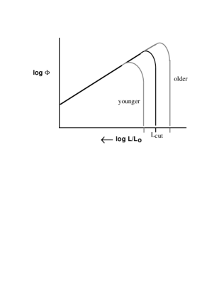
Figure 4: Schematic luminosity functions for populations of three different ages, from Kawaler ([1997]). This illustrates the case of a constant star formation rate with time, a Mestel cooling law ($t_{\rm cool}\propto L^{-5/7}$), and three disk ages.

the lower the luminosity of the cutoff. The stars populating the lowest luminosity bin are the oldest white dwarfs in the sample; with increasing age, they reach lower luminosity and pile up because of the lengthening cooling time scale.

When crystallization begins, the cooling rate temporarily slows, and the luminosity function will rise above the Mestel curve. Debye cooling will cause a drop in $\Phi$ with the associated accelerated cooling. Of course, realistic calculations of the luminosity function are needed for detailed comparison with the observed luminosity function.

Figure 5 shows a sample of realistic luminosity functions constructed using realistic white dwarf models computed (and kindly provided) by Matt Wood (described in Oswalt et al. [1996]). Note that the general slope of this cooling curve is nearly $-5/7$, but with a depression at high luminosities and a bump near the final cutoff. Also shown in Figure 5 is the observed luminosity function of Liebert et al. ([1988]). Agreement between the theoretical and observed luminosity functions above the drop–off is very good; those portions that disagree may result from changes in the star formation rate and/or the IMF over time. Such possibilities provide an intriguing use of the white dwarf luminosity function to explore the history of star formation in our galaxy (or, in the near future, in other stellar populations such as globular clusters).

Figure 5 clearly shows the effect of increasing age on the white dwarf luminosity function; older populations have fainter white dwarf stars. The low–luminosity cutoff decreases in luminosity with increasing population age; the figure shows luminosity functions for ages from 7 Gyr to 12 Gyr. Inspection of this figure reveals that the observed luminosity function is consistent with an age for the disk of the Milky Way of between 8 and 11 Gyr, with a best value of about 9 Gyr.

Figure 5: Theoretical white dwarf luminosity functions (constructed with DA white dwarf evolutionary sequences computed by Matt Wood) for several input disk ages. The drop–off in luminosity corresponds to disk ages from 7 Gyr (at the highest luminosity) to 12 Gyr. Also shown is the observed white dwarf luminosity function.

3.2 Sensitivity to the input physics

The derived age of the galactic disk depends on the input physics used in the computation of the white dwarf cooling rates. Given an observed, or otherwise fixed, luminosity function for comparison, the uncertainties in the derived ages follow from uncertainties in various properties of the white dwarf models. These properties, the sensitivity of the age to them, and the real range of possible ages, are summarized in Table 1. This table uses information from Winget & Van Horn ([1987]) and Wood ([1992]). It lists how the time for a white dwarf with a mass of $0.60M_{\odot}$ to drop to a luminosity of $10^{-4.4}L_{\odot}$ changes with various changes in the input physics.

Input physics (“$X$”)	$\frac{dt_{\rm disk}}{d\log X}$	real range
$m_{\rm helium}$	-0.7 Gyr	$\leq 1.4^{*}$ Gyr
$A_{\rm core}$ (C? O?)	-16 Gyr	$\approx 2^{*}$ Gyr
conductive opacity	+7.6 Gyr	$\leq 0.3$ Gyr
radiative opacity	+1.4 Gyr	$\leq 0.06$ Gyr
$Z_{\rm env}$	+1.4 Gyr	$\approx 0.2$ Gyr
fractionation	–	$<2$ Gyr
other stuff	?	$<1$ Gyr ?
∗ measurable with pulsation observations

Table 1: Dependence on $t_{\rm disk}$ on input physics

For example, if the mass of the surface helium layer is increased by one decade, the cooling time for a $0.60M_{\odot}$ white dwarf will decrease by 0.7 Gyr. In this tabulation, the values of $m_{\rm helium}$, $A_{\rm core}$, and $Z_{\rm env}$ are uncertain because of unknowns in the prior evolution of the white dwarf stars — they depend on how the star became a white dwarf star, on the ${}^{12}C(\alpha,\gamma)^{16}O$ nuclear reaction cross section, and on the trace metal content in white dwarf envelopes. The “real range” represents the current uncertainty in the cooling time given current uncertainties in the listed parameters. The dominant uncertainties arise from the thickness of the surface helium layer and on the core composition. The combination of these uncertainties yields a current best–estimate of the age of the galaxy of about $9.3\pm 1.5$ Gyr.

Fortunately, through observations of the pulsating white dwarf stars, there is a way to measure these quantities that is independent of approaches that use the observed luminosity function (see Kawaler [1997] for details). These observed pulsations allow us to measure the depth of subsurface transition zones and, therefore, the thickness of the surface helium layer in the pulsating DO and DB white dwarfs. Other pulsators place constraints on the core composition through the rate of period change.

4 The white dwarf luminosity function of the halo

As described earlier, the white dwarfs that are likely to appear on the HDF are halo white dwarfs. This section discusses the issues that need to be addressed to examine such a halo population.

4.1 Differences from the disk component

Nearly all of the work in the field so far has been on the white dwarf luminosity function of the Galactic disk, simply because that is where the observed white dwarfs live. When considering the white dwarf component of the galactic halo, however, many of the inputs into constructing theoretical WDLFs must be changed, based on what we know (or think we know) about stellar properties and star formation during the initial collapse of our galaxy.

4.1.1 Star formation rate: a burst

Whereas star formation has continued in the disk from the early history of the galaxy to the present, the stars of the halo formed over a very brief period very early on. Therefore, in modeling the WDLF for halo stars, a nearly universal assumption is that halo stars formed in a single burst at some time in the past (Tamanaha et al. [1990]). The time of this burst is the age of the oldest stellar component of the Milky Way.

With this assumption, the star formation rate $\psi(t_{h})$ becomes simply a constant, with a value equal to the total number of stars (of all masses) produced in the burst. Associated with this is the time $t_{h}$ of the burst; adjusting $t_{h}$ allows examination of how the WDLF depends on the halo age.

This simplifies the numerical calculation of the WDLF for the halo; if we consider the star formation rate such a $\delta$ function, then

$$-\frac{dN}{dM_{\rm b}}=\frac{\log(10)}{2.5}\;\psi(t_{h})\;\phi(M)\;\tau_{\rm cool}\left[\frac{dt_{\rm ms}}{dM_{\rm i}}+\frac{dt_{\rm cool}}{dM_{\rm wd}}\frac{dM_{\rm wd}}{dM_{\rm i}}\right]^{-1}$$ (4.8)

4.1.2 The initial mass function

Several lines of evidence point to an IMF for the halo that was quite different than the IMF of the disk. The observed scarcity of low–mass halo stars requires an IMF for halo stars (i.e. Bahcall et al. [1994]) that does not continue to rise at low mass (as does the Salpeter IMF for the disk). At the high-mass end, the disk IMF applied to the halo would have produced a higher metallicity (through supernovae) in halo stars than is observed (Ryu et al. [1990]). Thus the IMF for the halo is a function that is peaked at an intermediate mass.

Additional theoretical evidence leads to an IMF that is parameterized conveniently, following Adams & Laughlin ([1996]), as

$$\ln\left[\frac{dN}{dM}(\ln M)\right]=A-\frac{1}{2\sigma^{2}}\left[\ln\left(\frac{M}{m_{c}}\right)\right]^{2}$$ (4.9)

where the parameter $A$ is a normalization parameter, $\sigma$ characterizes the width of the distribution, and $m_{c}$ is related to the mass at the peak of the distribution. Adams & Laughlin ([1996]) choose base values for these parameters are $m_{c}=2.3$ and $\sigma=0.44$, though allowable values range from $m_{c}$ of 2.0 to 4.0 and $\sigma$ ranging from 0.10 to 0.40 for a halo population. They also show that for a disk population, the Population I IMF has values for these parameters closest to $\sigma=1.57$ and $m_{c}=0.15$.

4.1.3 The initial–final mass relation

The initial–final mass relation was derived empirically using Population I stars, typically in moderate–aged open clusters. Theoretical initial–final mass relations have reproduced the observed relation by imposing mass loss on the Asymptotic Giant Branch using a variety of uncertain mass–loss prescriptions. Because of the dependency of the initial–final mass loss relation on such mass loss, it is likely that the relationship will be different for the metal–poor progenitors of the halo white dwarfs.

Such low–metallicity stars will have envelope opacities that may be significantly smaller than their Pop I counterparts. The most likely mechanism driving mass loss on the AGB is radial pulsation (such as in Mira variables; see Bowen and Willson [1991]). If so, mass loss rates on the AGB for Pop II stars may have been smaller… leading to white dwarfs growing to much larger masses inside of them than Pop I stars. This would steepen the initial–final mass relation, and bring the lower–mass limit for Type II supernovae well below the 8 to 10 $M_{\odot}$ that it is for Population I.

4.2 Models of the halo WDLF

We now have all the ingredients we need to explore the shape of the WDLF for halo white dwarf stars. For more details about some of the results described in this section, see Tamanaha et al. ([1990]), Adams & Laughlin ([1996]), Chabrier et al. ([1996]), and Graff et al ([1998]). Here we assume a total number density of halo white dwarfs of $4\times 10^{-3}{\rm pc}^{-3}$, which corresponds to a mass density of approximately 25% of the dark halo.

Considering first the halo WDLF in isolation, the influence of the IMF on the WDLF is shown in Figure 6. For this figure, I used Wood’s DA white dwarf models to compute the halo WDLF using the equation shown above. All three curves correspond to a halo age of 12 Gyr, but with different values for the parameters governing the IMF. The heavy line shows the WDLF corresponding to the reference values of $m_{c}=2.3$ and $\sigma=0.44$. Narrowing the IMF by reducing $\sigma$ results in a narrower WDLF (compare the heavy and light lines in Figure 6), while increasing the value of $m_{c}$ shifts the WDLF to lower luminosities. For reference, the dotted line shows the WDLF using the IMF for the disk.

Figure 6: Theoretical WDLFs for halo models at 12 Gyr. The heavy solid line corresponds to an IMF with parameters $m_{c}=2.3$ and $\sigma=0.44$. A narrower IMF ($\sigma=0.24$) is shown as a thin line, and an IMF centered at higher mass is shown by a dashed line ($m_{c}=3.3$). The dotted line shows the halo WDLF assuming a disk IMF, for comparison.

The effect of the halo age on the WDLF of halo white dwarfs is similar to that of increasing $m_{c}$. Older halos produce WDLFs that reach lower luminosities with broader peaks. This is clearly a result of the fact that the white dwarf population has had more time to cool to lower luminosities. The entire distribution moves towards lower luminosity. In Figure 7, the evolution of the WDLF for a halo white dwarf population is clearly evident.

Figure 7: Theoretical WDLFs for halo models with fixed IMF parameters, and the same total space density, at ages of 10, 12, and 14 Gyr. The dotted lines are the complete WDLF including disk stars. The Liebert, et al. ([1988]) observed disk WDLF is also shown.

Under these circumstances, the older the halo, the greater the chance that halo white dwarfs may have escaped detection by current surveys. In addition, if the IMF for the halo is skewed towards higher mass stars at the expense of low mass stars (i.e. a larger $m_{c}$) then the halo portion of the composite WDLF will be forced to lower luminosity.

More complete discussions of the form of the halo WDLF can be found in the papers cited at the beginning of this subsection; Figures 6 and 7 should serve to illustrate the main points about the dependence of the halo WDLF on age and the IMF. For example, Adams & Laughlin ([1996]) explore a range of values of the parameters of the IMF (using pure carbon white dwarf models) – and the consequences for other observables including the residual gas left over after the mass loss that halo stars must have undergone in the production of halo white dwarfs. Graff et al. ([1998]) consider the effects of fractionation during crystallization on the halo WDLF, as well as the many selection effects associated with surveys, and the issue of the bolometric correction for such cool objects.

5 Observational constraints on halo white dwarfs

The MACHO results have already been discussed, and are provocative indeed. There is a firm upper limit on the number of halo white dwarfs: the total mass of halo white dwarfs must not exceed the mass of the galactic halo! At or near the position of the Sun, then, the halo white dwarf density must be less than about $1.7\times 10^{-2}{\rm pc}^{-3}$. This is a very large number that exceeds (by nearly an order of magnitude) the density of white dwarfs currently known. Interestingly, if halo white dwarfs are to account for a significant fraction of the halo mass, then the number density cannot be significantly lower than this. Thus if the MACHO interpretation of their data is correct, such white dwarfs must have escaped detection by current surveys.

5.1 Presence (or absence) of halo white dwarfs in existing white dwarf surveys

How do studies of the white dwarf luminosity function that were restricted to the solar neighborhood constrain the halo WDLF? This issue has been addressed by Adams & Laughlin ([1996]) who show how the luminosity function of white dwarfs in the solar neighborhood as reported by Liebert et al. (1988) limits the number density of halo white dwarfs. The last data point in the disk WDLF is an upper limit of approximately $6\times 10^{-5}$pc${}^{-3}M_{\rm bol}^{-1}$ at $\log L=-4.7$. For luminosity functions that derive from standard models of cooling white dwarfs, Adams & Laughlin (1996) show that their luminosity function must quickly rise to several $\times 10^{-4}$pc${}^{-3}M_{\rm bol}^{-1}$ and remain high down to very low luminosities if the age of this population is not excessively larger than the age of the oldest globular clusters.

This is apparent from examination of Figure 7, which compares the WDLF to a “standard” computation of the WDLF including a halo population. At $\log L=-4.7$, the theoretical WDLF lies above the observed upper limit for all halo ages, using the most likely parameters of the IMF. Recall that these theoretical WDLF calculations assume that the total mass of halo white dwarfs is 25% of the total halo mass. To be consistent with the last WDLF point from Liebert et al. ([1988]), the contribution of white dwarfs to the mass of the halo must be much less than 25%.

The fraction of the halo mass contributed by white dwarfs can be greater if the width of the IMF is much narrower than $\sigma=0.44$, as shown in Figure 6. If $\sigma=0.24$ then a halo age of 14 Gyr can have a white dwarf contribution of 25% and still be consistent with the lowest luminosity WDLF point. Thus the IMF width must be extremely narrow for the halo white dwarfs to contribute significantly to the mass of the halo and to have largely escaped detection in traditional searches for white dwarfs. This one of the essential points made by Adams & Laughlin ([1996]) and Graff et al. ([1998]).

With this constraint alone, the interpretation of lensing events in the MACHO project as white dwarfs requires a halo age of 14 Gyr or more along with a rapid rise in the luminosity function at lower luminosities. Can this prediction be addressed by the HDF? Read on…

5.2 White dwarfs (or lack thereof) on the HDF

If, as suggested by the MACHO results, the halo dark matter of the Milky Way is up to 50% (by mass) halo white dwarfs, then up to half of the halo mass sampled in the HDF can be white dwarf stars. The mass sampled is dependent on the minimum absolute magnitudes of these halo white dwarfs and the magnitude limit of the images. Kawaler ([1996]) computes the expected number of white dwarfs on the HDF at any magnitude with minimal assumptions about the WDLF and the magnitude distribution of halo white dwarfs. Following Adams & Laughlin ([1996]), this section will describe more precisely the way that the WDLF of the halo is affected at different luminosities by the result of searches for white dwarfs on the HDF.

Despite heroic efforts at finding them, there are few obvious stars in the HDF images (apart from a few “bright” 20th magnitude stars); the task of discriminating between stellar and nonstellar objects at very faint magnitudes requires extreme care (see the review by John Bahcall in this volume). For example, Flynn et al. ([1996]) report that no white dwarfs exist down to $V=26.3$ for objects with $2.5>V-I>1.8$. They do find bluer stellar objects ($V-I$ between 0 and 1.8) that are consistent in number as well as color with low–mass main sequence stars. Similar results have been reported by Mendez et al. ([1996]). Thus it appears that there are no white dwarfs on the HDF down to $V<28$ or so. As discussed by Flynn et al. ([1996]) and by Bahcall (these proceedings), confident discrimination of true stellar objects from compact faint galaxies is not possible at higher magnitudes on the HDF.

While disappointing, this upper limit still important when trying to constrain the white dwarf population of the halo. We can use it to further constrain the shape of the WDLF at very low luminosities. Here we use equation (1.2) from the Introduction; this equation shows the volume sampled by the HDF given these figures, and allows calculation of an upper limit to the space density of white dwarf stars at each luminosity bin. For simplicity, we consider as an upper limits to the space density $1/V$, with $V$ determined with equation 1.2, and zero bolometric correction (but see Graff et al. [1998]). This then gives the upper limit for white dwarfs based on the HDF null result as

$$\log\Phi_{\rm up}=-6.80-0.6m_{V,{\rm lim}}-1.5\log\left(\frac{L}{L_{\odot}}\right)\;.$$ (5.10)

For each magnitude fainter that searches for white dwarfs on the HDF can go, the WDLF upper limit drops by 0.6 dex at a given luminosity.

Figure 8 shows the HDF limit on the halo contribution (as a dotted line, assuming a limiting magnitude of $V=28$) to the WDLF along with several models of the WDLF and the data for disk white dwarfs. In Figure 8, as earlier, the models are for a halo white dwarf population with a total mass equal to 25% of the mass of the dark halo. Each panel represents model WDLFs with the same disk age (9 Gyr) and halo ages of 12 Gyr and 14 Gyr, with the 14 Gyr luminosity function lying to the right in all three panels. As can be surmised by examining Figure 7, a halo age of 10 Gyr is clearly inconsistent with the data in all cases.

Figure 8: The WDLF for the disk + halo. The data points are the observed disk WDLF from Liebert et al. ([1988]); the dotted line represents an upper limit based on the lack of white dwarfs on the HDF (assuming a magnitude limit of $V=28$. Solid lines represent theoretical WDLFs for DA white dwarfs with a disk age of 9 Gyr, and halo ages of 12 Gyr and 14 Gyr. Older models reach lower luminosities. The three panels represent different parameters for the IMF. In comparison with the top panel, the middle panel shows results for an IMF with a higher central mass, while the bottom panel represnts an IMF with a much narrower width. All models assume a halo white dwarf mass equal to 25% of the total mass of the dark halo.

The top panel of Figure 8 shows the model WDLF using the fiducial parameters for the IMF. While the WDLF falls below the HDF limit for both ages, the lowest luminosity disk WDLF points are clearly inconsistent with the theory. Shifting the IMF to higher masses, as illustrated by the middle panel of Figure 8, helps drop the theoretical WDLF near the disk cutoff, but is still inconsistent with the observations. The bottom panel illustrates that the only way for a halo WDLF to satisfy the constraints of the disk observations and the HDF is to narrow the IMF. Bringing the width parameter down to $\sigma=0.24$ satisfies both constraints for a halo age of 14 Gyr and older. As the trend in Figure 8 shows, a younger halo with a narrower distribution might satisfy the disk constraints, but would then rise above the HDF upper limit at slightly lower luminosities than the disk cutoff. Another point to consider is that the models used to construct the WDLFs in Figure 8 do not include the effects of fractionation of the crystallizing white dwarf cores. Graff et al. ([1998]) point out that the such an effect increases the age constraints by about 2 Gyr.

There are a variety of other ways to compute the theoretical halo WDLF to address the observations. Again, the reader is urged to consult the papers by Tamanaha et al. ([1990]), Adams & Laughlin ([1996]) and Graff et al ([1998]) for more details of the influence of various parameters on the halo white dwarf luminosity function.

The results presented in Figure 8 are intended to be representative and schematic. They show the essential results of the lack of finding white dwarfs on the HDF. First, the lack of white dwarfs on the HDF is not a surprise given what we have learned from studies of the white dwarf luminosity function of the galactic disk. Second, the contribution of white dwarfs to the Milky Way’s massive dark halo can be limited based on this lack of detection. For reasonable parameters for the halo white dwarf population, it is difficult for this null result on the HDF (and the disk WDLF) to be consistent with a halo comprised of more than 25% white dwarfs by mass. Third, if the limits of the HDF (or other very deep surveys) can be pushed fainter, the MACHO results require that some white dwarfs should be found (probably with an $M_{\rm bol}$ of about 17.5 to 19). Finally, we can hope to learn a great deal about halo white dwarfs by their discovery in abundance, even if it is not a chore for which HST is ideally suited.

5.3 Postscript: white dwarfs on the HDF – sort of

In closing, the results of the WDLF studies of the disk of our galaxy, along with the newer work on white dwarfs in the halo, allow us to estimate the total number of white dwarfs in the Milky Way. Assuming a uniform distribution of white dwarf stars in the galactic disk, the local density implies that there are approximately $3\times 10^{9}$ white dwarfs in the disk. We can then use the luminosity function of the disk to estimate the total luminosity from all of these white dwarf stars as approximately $3\times 10^{6}L_{\odot}$. Thus, to ballpark accuracy, white dwarfs contribute a fraction of about $3\times 10^{-5}$ of the total photon luminosity of our galaxy.

If we take the Milky Way as representative of the galaxies seen on the HDF, we can ask how many photons that were counted by the HDF originated on a white dwarf in a galaxy. Given the number of galaxies on the HDF and the total photon count, approximately 1 photon per galaxy came from a white dwarf. Therefore, white dwarfs have indeed been detected by the HDF; the trick remains identifying which of those photons came from which white dwarf!