COSMIC AXIONS

The current cosmological constraints on a dark matter axion are reviewed. We describe the basic mechanisms by which axions are created in the early universe, both in the standard thermal scenario in which axion strings form and in inflationary models. In the thermal scenario, the dominant process for axion production is through the radiative decay of an axion string network, which implies a dark matter axion of mass $m_{\rm a}\sim 100\,\mu\hbox{\rm eV}$ with specified large uncertainties. An inflationary phase does not affect this string bound if the reheat temperature is high $T_{\rm reh}\hbox{${\lower 1.37775pt\hbox{$>$}\atop\raise 0.48221pt\hbox{$\sim$}}$}f_{\rm a}$ or, conversely, for $T_{\rm reh}\hbox{${\lower 1.37775pt\hbox{$<$}\atop\raise 0.48221pt\hbox{$\sim$}}$}f_{\rm a}$, if the Hubble parameter during inflation is large $H_{1}>f_{\rm a}$; in both cases, strings form and we return to the standard picture with a $m_{\rm a}\sim 100\,\mu\hbox{\rm eV}$ dark matter axion. Inflationary models with $f_{\rm a}>H_{1}>T_{\rm reh}$ face strong CMBR constraints and require ‘anthropic misalignment’ fine-tuning in order to produce a dark matter axion; in this case, some inflation models are essentially incompatible with a detectable axion, while others can be engineered to allow a dark matter axion anywhere in a huge mass range below $m_{\rm a}\hbox{${\lower 1.37775pt\hbox{$<$}\atop\raise 0.48221pt\hbox{$\sim$}}$}1$meV. We endeavour to clarify the sometimes confusing and contradictory literature on axion cosmology.

1 Introduction

The axion has consistently remained one of the most popular dark matter candidates ever since the early 1980’s. Unlike many other more exotic particles, the axion’s existence depends only on a minimal extension of the standard model $\!{}^{{\bf?},{\bf?}}$ which also solves one of its key difficulties—the strong CP problem of QCD. In the standard thermal scenario, cosmic axions are created primarily through the radiative decay of a network of axion strings $\!{}^{{\bf?},{\bf?}}$ formed in the early universe at $t\approx 10^{-25}$s; this network rapidly annihilates when the axion mass ‘switches on’ at $t\approx 10^{-4}$s leaving no trace except for a background of cosmic axions. If these axions are to be the dark matter of the universe, then their mass must be about $m_{\rm a}\sim 100\mu\hbox{eV}$ (with significant uncertainties). $\!{}^{{\bf?}}$ On the other hand, if an inflationary phase in the early universe eliminates all axions strings with a low reheat temperature, then dark matter axions are created by more quiescent mechanisms $\!{}^{{\bf?}}$ and they can have any mass below $\!{}^{{\bf?}}$ $m_{\rm a}\hbox{${\lower 1.72218pt\hbox{$<$}\atop\raise 0.60275pt\hbox{$\sim$}}$}1$meV. Astrophysical constraints on the axion mass $\!{}^{{\bf?},{\bf?}}$ suggest that $m_{\rm a}\hbox{${\lower 1.72218pt\hbox{$<$}\atop\raise 0.60275pt\hbox{$\sim$}}$}10\,\hbox{\rm meV}$, so a viable parameter window exists for the dark matter axion; the only doubt that remains is what it actually should weigh.

Present large-scale axion search experiments $\!{}^{{\bf?},{\bf?}}$ are focussing on a mass range, $m_{a}\sim 1\hbox{--}10\,\mu\hbox{\rm eV}$, for a variety of historical and technological reasons. However, a number of proposed experiments may have the sensitivity to look for the heavier dark matter axion of the standard thermal scenario, $\!{}^{{\bf?}}$ which appears to have a better motivated mass prediction. This axion cosmology overview, then, keeps this missing matter quest to the forefront. Our primary focus is not on the viable axion mass range, but rather on cosmological predictions of the mass of a dark matter axion, that is, an axion for which $\Omega_{\rm a}$ is of order unity.

2 Axion properties and constraints

The standard model of particle physics, based around the Weinberg-Salam model for electroweak interactions and QCD for strong interactions, has one significant flaw—the strong CP problem: non-perturbative effects of instantons add an extra term to the perturbative Lagrangian and the coefficient of this term, denoted $\theta$, governs the level of CP violation in QCD. The absence of any such violation in all observed strong interactions imposes a constraint on $\theta$, the most stringent being $\theta<10^{-10}$ due to the absence of a neutron electric dipole moment. $\!{}^{{\bf?}}$ Since the value of $\theta$ is effectively arbitrary, one is left with a severe fine tuning problem.

The elegant solution of Peccei and Quinn $\!{}^{{\bf?}}$ is to allow $\theta$ to become a dynamical field which relaxes toward the CP conserving value $\theta=0$  through the spontaneous breaking of a $U(1)$-symmetry. Essentially, $\theta$ becomes the phase of a complex scalar field $\phi=|\phi|\exp(i\theta)$, which takes a non-zero expectation value at the Peccei-Quinn scale $f_{\rm a}$, that is, it has a potential of the general form,

$$V(\phi)={\lambda\over 4}(|\phi|^{2}-f_{\rm a}^{2})^{2}+{f_{\pi}^{2}m_{\pi}^{2}}{|\phi|\over f_{\rm a}}(1-\cos\theta)\,.$$ (1)

The azimuthal particle excitation in the $\theta$-direction (around the bottom of the ‘Mexican hat’) is a pseudo-Goldstone boson $\!{}^{{\bf?}}$—the axion field $a=f_{\rm a}\theta$. Here, the second term in the potential gives a small mass $m_{\rm a}$ to the axion, however, note that this mass $m_{\rm a}(T)$ only ‘switches on’ through instanton effects at the QCD-scale $\Lambda_{\rm QCD}\approx 200$MeV (that is, $m_{\rm a}(T)\approx 0$, $T>\!>\Lambda_{\rm QCD}$ and $m_{\rm a}(T)=m_{\rm a},\,\hbox{const.}$, $T<\!<\Lambda_{\rm QCD}$). This ensures that the $\phi$-field lies in the true CP-conserving minimum $\theta=0$ at late times. Throughout this discussion, we consider the simplest $N=1$ axion which couples to a single quark and has a unique vacuum. Later, we shall comment on the $N>1$ axion with a $\cos N\theta$ potential, noting the implications of the additional vacuum degeneracy.

The axion has an extremely small mass $m_{\rm a}$ which is inversely proportional to the Peccei-Quinn scale $f_{\rm a}$,

$$m_{\rm a}=6.2\times 10^{-6}\hbox{eV}\left(10^{12}\hbox{GeV}\over f_{\rm a}\right)\,.$$ (2)

The axion couplings to ordinary matter also scale as $f_{\rm a}^{-1}$, specifically to nucleons $g_{\rm aN}=C_{\rm N}m_{\rm N}/f_{\rm a}$ (${\rm N=n,\,p}$) and to photons $g_{\rm a\gamma}=(\alpha/2\pi f_{\rm a})(C_{\gamma}-1.9)$ where $C_{\rm N}$ and $C_{\gamma}$ are parameters of order unity. These expressions do not adequately encompass the model-dependencies of axion phenomenology which includes, for example, the DFSZ axion with a tree-level coupling to the electron and the KSVZ axion with none (refer to a review such as ref. [14]).

Initially, it was supposed that the Peccei-Quinn scale was close to the electroweak phase transition $f_{\rm a}\sim T_{\rm EW}$, but an exhaustive search of accelerator data ruled out this possibility, implying $f_{\rm a}\hbox{${\lower 1.72218pt\hbox{$>$}\atop\raise 0.60275pt\hbox{$\sim$}}$}10^{7}{\rm GeV}$. However, the ensuing disappointment was short-lived because there is no phenomenological reason why the Peccei-Quinn scale $f_{\rm a}$ could not be much higher, even up to grand-unification scales. Thus, the ‘invisible’ axion was born, an extremely light particle with almost undetectably weak couplings of order $f_{\rm a}^{-1}$.

Accelerator limits on the new ‘invisible’ axion were soon superseded by astrophysical calculations of stellar cooling rates. Axions, being weakly coupled, can escape from the whole volume of a star and, in certain parameter ranges, this can exceed the usual heat loss mechanisms through convection and other surface effects. The oft-quoted ‘red giant limit’ on the axion $\!{}^{{\bf?}}$ is actually slightly weaker than that obtained from old globular cluster stars, $\!{}^{{\bf?}}$ $m_{\rm a}\hbox{${\lower 1.72218pt\hbox{$<$}\atop\raise 0.60275pt\hbox{$\sim$}}$}0.4$eV or $f_{\rm a}\hbox{${\lower 1.72218pt\hbox{$>$}\atop\raise 0.60275pt\hbox{$\sim$}}$}2\times 10^{7}$. However, more stringent constraints come from supernova 1987a; the duration of the observed neutrino signal, associated with nascent neutron star cooling, depends on the axion-nucleon coupling $g_{\rm aN}$. Originally, a strong bound $m_{\rm a}\hbox{${\lower 1.72218pt\hbox{$<$}\atop\raise 0.60275pt\hbox{$\sim$}}$}1$meV was proposed, $\!{}^{{\bf?}}$ but this did not adequately reflect the model-dependence of axion phenomenology. More conservative estimates in realistic axion models yield the overall bound $\!{}^{{\bf?}}$

$$m_{\rm a}~{}\hbox{${\lower 1.72218pt\hbox{$<$}\atop\raise 0.60275pt\hbox{$\sim$}}$}~{}10\,\hbox{meV}\,,\qquad f_{\rm a}~{}\hbox{${\lower 1.72218pt\hbox{$>$}\atop\raise 0.60275pt\hbox{$\sim$}}$}~{}10^{9}\hbox{GeV}\,.$$ (3)

Note that significant uncertainties remain for all these astrophysical constraints and recent reviews should be consulted such as refs. [7,8]. Interestingly, astrophysics seems to have no impact in any cosmological scenario on the viable mass range of a dark matter axion.

3 Standard thermal axion cosmology

The cosmology of the axion is determined by the two energy scales $f_{\rm a}$ and $\Lambda_{\rm QCD}$. The first important event is the Peccei-Quinn phase transition which is broken at a high temperature $T\sim f_{\rm a}\hbox{${\lower 1.72218pt\hbox{$>$}\atop\raise 0.60275pt\hbox{$\sim$}}$}10^{9}$GeV by (3). This creates the axion, at this stage effectively massless, as well as a network of axion strings $\!{}^{{\bf?}}$ which decays gradually into a background cosmic axions. $\!{}^{{\bf?},{\bf?}}$ One can, in principle, engineer models in which an inflationary epoch interferes with the effects of the Peccei-Quinn phase transition, but we shall deal with this case in the next section, focussing first on this ‘standard thermal scenario’. At a much lower temperature $T\sim\Lambda_{\rm QCD}$ after axion and string formation, instanton effects ‘switch on’, the axions acquire a small mass, domain walls form $\!{}^{{\bf?}}$ between the strings $\!{}^{{\bf?}}$ and the complex hybrid network annihilates in about one Hubble time. $\!{}^{{\bf?}}$ In the cold dark matter scenario of interest here, the remaining axions redshift and eventually dominate the energy density of the universe at equal matter-radiation $t_{\rm eq}$.

There are three possible mechanisms by which axions are produced in the ‘standard thermal scenario’: (i) thermal production, (ii) axion string radiation and (iii) hybrid defect annihilation when $T=\Lambda_{QCD}$. Axions consistent with the bound (3) decouple from thermal equilibrium very early at a temperature $\!{}^{{\bf?}}$ $T_{\rm d}\hbox{${\lower 1.72218pt\hbox{$>$}\atop\raise 0.60275pt\hbox{$\sim$}}$}4\times 10^{5}$GeV; their subsequent history and number density is analogous to the decoupled neutrino, except that unlike a 100eV massive neutrino, thermal axions cannot hope to dominate the universe with $m_{\rm a}\hbox{${\lower 1.72218pt\hbox{$<$}\atop\raise 0.60275pt\hbox{$\sim$}}$}10$meV. Thermal production can still continue down to about $\Lambda_{\rm QCD}$ but this contribution is subdominant in light of the astrophysical bound (3). We now turn to the two dominant axion production mechanisms, but first we address an important historical digression.

3.1 Misalignment misconceptions

The original papers on axions suggested that axion production primarily occurred, not through the above mechanisms, but instead by ‘misalignment’ effects at the QCD phase transition.  $\!{}^{{\bf?},{\bf?}}$ As applied to the thermal scenario, this turned out to be a very considerable underestimate, but it is useful to recount the argument and its flaws because they are often repeated in the literature. Before the axion mass ‘switches on’, the axion field takes random values throughout space in the range 0 to $2\pi$. However, afterwards the true minimum becomes $\theta=0$, so the field in the ‘misalignment’ picture begins to coherently oscillate about this minimum; this homogeneous mode corresponds to the ‘creation’ of zero momentum axions. Given an initial rms value $\theta_{\rm i}$ for these oscillations, it is relatively straightforward to estimate the total energy density in zero momentum axions and compare to the present mass density of the universe (assuming a flat $\Omega=1$ FRW cosmology): $\!{}^{{\bf?},{\bf?},{\bf?}}$

$$\Omega_{{\rm a},{\rm h}}~{}\approx~{}0.2\,\Delta h^{-2}\;\theta_{\rm i}^{2}{\rm f}(\theta_{\rm i})\,\bigg{(}{f_{\rm a}\over 10^{12}{\rm GeV}}\bigg{)}^{1.18}\approx~{}2\,\Delta h^{-2}\;\theta_{\rm i}^{2}{\rm f}(\theta_{\rm i})\,\bigg{(}{10^{-6}{\rm eV}\over m_{\rm a}}\bigg{)}^{1.18}$$ (4)

where $\Delta\approx 3^{\pm 1}$ accounts for model-dependent axion uncertainties, as well as those due to the nature of the QCD phase transition, and $h$ is the rescaled Hubble parameter. The function ${\rm f}(\theta)$ is an anharmonic correction $\!{}^{{\bf?}}$ for fields near the top of the potential close to unstable equilibrium $\theta\approx\pi$, that is, with ${\rm f}(0)=1$ at the base $\theta\approx 0$ and slowly diverging approximately as $\!{}^{{\bf?}}$ ${\rm f}(\theta)\sim-\ln(|\pi-\theta|)$ for $\theta\rightarrow\pi$. If valid, the estimate (4) would imply a constraint $\!{}^{{\bf?},{\bf?}}$ $f_{\rm a}\hbox{${\lower 1.72218pt\hbox{$<$}\atop\raise 0.60275pt\hbox{$\sim$}}$}10^{12}{\rm GeV}\,,$ $m_{\rm a}\hbox{${\lower 1.72218pt\hbox{$>$}\atop\raise 0.60275pt\hbox{$\sim$}}$}5\mu{\rm eV}$ for the anticipated thermal initial conditions with $\theta_{\rm i}={\cal O}(1)$ (suggested to be $\theta_{\rm i}=\pi/\sqrt{3}$).

In the thermal scenario, however, the expression (4) has three serious shortcomings: (i) The axions are not ‘created’ by the mass ‘switch on’ at $t=t_{QCD}$, they are already there with a specific momentum spectrum $g(k)$. Dynamical mechanisms prior to this time—thermal effects, string radiation and field realignment—will have created this axion spectrum. Because correlations cannot be established acausally, there will be a lower cutoff to the axion momenta set by the horizon, $k_{\rm min}^{-1}\sim t$; only inflationary models can have truly zero momentum axions. The actual axion number obtained from $g(k)$ is clearly much larger than an rms average in (4) which ignores the true particle content. (ii) Secondly, this estimate was derived before much stronger topological effects were realized, notably the presence of axion strings and domain walls. These nonlinear effects complicate the oscillatory behaviour of $\theta$ considerably, implying that the homogeneous estimate (4) is poorly motivated. (iii) Finally, from a more general perspective, the expression (4) with $f_{\rm a}>\!>10^{12}$GeV seems to imply that axion mass ‘switch on’ changes the topology of the universe, taking us to an $\Omega>1$ closed model! Of course, this is not what happens, since the extrapolation breaks down and in reality the axions merely dominate the universe much earlier than $t_{\rm eq}$; we end up with an $\Omega_{\rm a}\rightarrow 1$ model with an unacceptably low baryon-to-axion ratio. $\!{}^{{\bf?}}$

3.2 Axion string network decay

Axions and axion strings are inextricably intertwined. Like ordinary superconductors or superfluid ⁴He, axion models contain a broken $U(1)$-symmetry and so there exist vortex-line solutions. Combine this fact with the Peccei-Quinn phase transition, which means the field is uncorrelated beyond the horizon, and a random network of axion strings must inevitably form. An axion string corresponds to a non-trivial winding from $0$ to $2\pi$ of the axion field $\theta$ around the bottom of the ‘Mexican hat’ potential (1). It is a global string with long-range fields, so its energy per unit length $\mu$ has a logarithmic divergence which is cut-off by the string curvature radius $R\hbox{${\lower 1.72218pt\hbox{$<$}\atop\raise 0.60275pt\hbox{$\sim$}}$}t$, that is,

$$\mu\approx 2\pi f_{\rm a}^{2}\ln(t/\delta)\,,$$ (5)

where the string core width is $\delta\approx f_{\rm a}^{-1}$ (taking $\lambda\approx{\cal O}(1)$ in (1)). By observing the logarithmic dependence in (5), the axion string might be interpreted as a delocalised ‘cloud of energy’, but on cosmological scales it is anything but non-local; if we have a string stretching across the horizon at the QCD temperature, then $\ln(t/\delta)\sim 65$ and over 95% of its energy lies within a tight cylinder enclosing only 0.1% of the horizon volume. To first order, then, the string behaves like a local cosmic string, a fact that can be established by a precise analytic derivation and careful comparison with numerical simulations. 

After formation and a short period of damped evolution, the axion string network will evolve towards a scale-invariant regime with a fixed number of strings crossing each horizon volume (for a cosmic string review see ref. [33]). This gradual demise of the network is achieved by the production of small loops which oscillate relativistically and radiate primarily into axions. The overall density of strings splits neatly into two distinct parts, long strings with length $\ell>t$ and a population of small loops $\ell<t$,

$$\rho=\rho_{\infty}+\rho_{L}\,.$$ (6)

High resolution numerical simulations $\!{}^{{\bf?},{\bf?}}$ confirm this picture of string evolution and suggest that the long string density during the radiation era is $\rho_{\infty}\approx 13\mu/t^{2}$. To date, analytic descriptions of the loop distribution have used the well-known string ‘one scale’ model, which predicts a number density of loops defined as $\mu\ell\,n(\ell,t)\,d\ell=\rho_{L}(\ell,t)d\ell$ in the interval $\ell$ to $\ell+d\ell$ to be given by $\!{}^{{\bf?}}$

$$n(\ell,t)={4\alpha^{1/2}(1+\kappa/\alpha)^{3/2}\over(\ell+\kappa t)^{5/2}t^{3/2}}\,,$$ (7)

where $\alpha$ is the typical loop creation size relative to the horizon and $\kappa\approx 65/[2\pi\ln(t/\delta)]$ is the loop radiation rate. Once formed at $t=t_{0}$ with length $\ell_{0}$, a typical loop shrinks linearly as it decays into axions $\ell=\ell_{0}-\kappa(t-t_{0})$. The key uncertainty in this treatment is the loop creation size $\alpha$, but compelling heuristic arguments place it near the radiative backreaction scale, $\alpha\sim\kappa$.

String loops oscillate with a period $T=\ell/2$ and radiate into harmonics of this frequency (labelled by $n$), just like other classical sources. Unless a loop has a particularly degenerate trajectory, it will have a radiation spectrum $P_{n}\propto n^{-q}$ with a spectral index $q>4/3$, that is, the spectrum is dominated by the lowest available modes. Given the loop density (7), we can then calculate the spectral number density of axions,

$${dn_{\rm a}\over d\omega}(t)\approx{350\alpha^{1/2}(1+\kappa/\alpha)^{3/2}f_{\rm a}^{2}\over\kappa^{3/2}\omega^{2}t^{2}}\left[1-\left(1+{\alpha\over\kappa}\right)^{-3/2}\right]\,,$$ (8)

which is essentially independent of the exact loop radiation spectrum provided $q>4/3$. From this expression we can integrate over $\omega$ to find the total axion number at the time $t_{\rm QCD}$, that is, when the axion mass ‘switches on’ and the string network annihilates. Subsequently, the axion number will be conserved, so we can find the number-to-entropy ratio and project forward to the present day. Multiplying the present number density by the axion mass $m_{\rm a}$ will give us the overall string contribution to the density of the universe: $\!{}^{{\bf?}}$

$$\Omega_{\rm a,\ell}\approx 11\Delta h^{-2}\bigg{[}\bigg{(}1+{\alpha\over\kappa}\bigg{)}^{3/2}-1\bigg{]}\bigg{(}{f_{\rm a}\over 10^{12}{\rm GeV}}\bigg{)}^{1.18}\,.$$ (9)

For the expected ratio $\alpha/\kappa\approx 1$, the axion contribution arising from direct radiation from long strings is an order of magnitude smaller than $\Omega_{\rm a,\ell}$, but it slightly reinforces (9). $\!{}^{{\bf?}}$ We note also that $\Omega_{\rm a,\ell}$ is well over an order of magnitude larger than the ‘misalignment’ estimate (4). The key additional uncertainty from the string model is the ratio $\alpha/\kappa$, which should be clearly distinguished from particle physics and cosmological uncertainties inherent in $\Delta$ and $h$, and appearing in other estimates of $\Omega_{\rm a}$. With a Hubble parameter near $h=0.5$, the string estimate (9) tends to favour a dark matter axion with a mass $m_{\rm a}\sim 100\mu$eV, as we shall discuss in the conclusion.

3.3 Axion mass ‘switch on’ and hybrid defect annihilation

Near the QCD phase transition the axion acquires a mass and network evolution alters dramatically because domain walls form. $\!{}^{{\bf?},{\bf?}}$ Large field variations around the strings collapse into these domain walls, which subsequently begin to dominate over the string dynamics. This occurs when the wall surface tension $\sigma$ becomes comparable to the string tension due to the typical curvature $\sigma\sim\mu/t$. The demise of the hybrid string–wall network proceeds rapidly, as demonstrated numerically. $\!{}^{{\bf?},{\bf?}}$ The strings frequently intersect and intercommute with the walls, effectively ‘slicing up’ the network into small oscillating walls bounded by string loops. Multiple self-intersections will reduce these pieces in size until the strings dominate the dynamics again and decay continues through axion emission.

An order-of-magnitude estimate of the demise of the string–domain wall network $\!{}^{{\bf?}}$ indicates that there is an additional contribution

$$\Omega_{\rm a,dw}\sim{\cal O}(1)\Delta h^{-2}\bigg{(}{f_{\rm a}\over 10^{12}{\rm GeV}}\bigg{)}^{1.18}\,.$$ (10)

This ‘domain wall’ contribution is ultimately due to loops which are created at the time $\sim t_{\rm QCD}$. Although the resulting loop density will be similar to (7), there is not the same accumulation from early times, so it is likely to be subdominant $\!{}^{{\bf?}}$ relative to (9). More recent work, $\!{}^{{\bf?}}$ questions this picture by suggesting that the walls stretching between long strings dominate and will produce a contribution anywhere in the wide range $\Omega_{\rm a,dw}\sim(1\hbox{--}44)\Omega_{\rm a,\ell}$; however, this assertion definitely requires further quantitative study. Overall, the domain wall contribution will serve to further strengthen the string bound (9) on the axion.

We note briefly that it is possible to weaken any axion mass bound through catastrophic entropy production between the QCD-scale and nucleosynthesis, that is, in the timescale range $10^{-4}s\hbox{${\lower 1.72218pt\hbox{$<$}\atop\raise 0.60275pt\hbox{$\sim$}}$}t_{\rm ent}\hbox{${\lower 1.72218pt\hbox{$<$}\atop\raise 0.60275pt\hbox{$\sim$}}$}10^{-2}s$. The idea has been suggested in a number of contexts, $\!{}^{{\bf?},{\bf?}}$ but these usually involve the energy density of the universe becoming temporarily dominated by an exotic massive particle with a tuned decay timescale.

4 Inflationary scenarios

The relationship between inflation and dark matter axions is enigmatic. Its significance depends on the magnitude of the Peccei-Quinn scale $f_{\rm a}$ relative to two key inflationary parameters, (i) the reheat temperature of the universe $T_{\rm reh}$ at the end of inflation and (ii) the Hubble parameter $H_{1}$ as the observed universe first exits the horizon during inflation. Inflation is irrelevant to the axion if $T_{\rm reh}\hbox{${\lower 1.72218pt\hbox{$>$}\atop\raise 0.60275pt\hbox{$\sim$}}$}f_{\rm a}$ because, in this case, the PQ-symmetry is restored and the universe returns to the ‘standard thermal scenario’ in which axion strings form and the estimate (9) pertains. Even if the reheat temperature is low $T_{\rm reh}<f_{\rm a}$, however, inflation will again be irrelevant if $H_{1}>f_{\rm a}$ because axion strings will form towards the end of inflation and we will return to a modified ‘standard thermal scenario’—as we shall discuss.

Thus, for inflation to impact the viability of a dark matter axion we must have $f_{\rm a}\hbox{${\lower 1.72218pt\hbox{$>$}\atop\raise 0.60275pt\hbox{$\sim$}}$}H_{1}\hbox{${\lower 1.72218pt\hbox{$>$}\atop\raise 0.60275pt\hbox{$\sim$}}$}T_{\rm reh}$, that is, inflation must occur at a low energy scale or we must have an extremely light axion. Inflation, in this case, essentially makes no prediction as to the axion mass. Like much in axion cosmology, these facts are not widely appreciated, so they deserve some case-by-case unravelling.

4.1 $H_{1}<f_{\rm a}$: Anthropic misalignment and quantum fluctuations

In an inflationary model for which $f_{\rm a}>H_{1}>T_{\rm reh}$, the $\theta$-parameter or axion angle will be set homogeneously over large inflationary domains before inflation finishes. $\!{}^{{\bf?}}$ In this case, the whole observable universe emerges from a single Hubble volume in which this parameter has some fixed initial value $\theta_{\rm i}$. Because the axion remains out of thermal equilibrium for large $f_{\rm a}$, subsequent evolution and reheating does not disturb $\theta_{\rm i}$ until the axion mass ‘switches on’ at $T\sim\Lambda_{\rm QCD}$. Afterwards, the field begins to oscillate coherently, because it is misaligned by the angle $\theta_{\rm i}$ from the true minimum $\theta=0$. This homogeneous mode corresponds to a background of zero momentum axions and it is the one circumstance under which the misalignment formula (4) actually gives an accurate estimate of the relative axion density $\Omega_{\rm a}$.

By considering the dependence $\Omega_{\rm a,h}\propto\theta_{\rm i}^{2}$ in (4), we see that inflation models have an intrinsic arbitrariness given by the different random magnitudes of $\theta_{\rm i}$ in different inflationary domains. $\!{}^{{\bf?}}$ While a large value of $f_{\rm a}>\!>10^{12}$GeV might have been thought to be observationally excluded, it can actually be accommodated in domains where $\theta_{\rm i}<\!<1$. This may seem highly unlikely but, if we consider an infinite inflationary manifold or a multiple universe scenario including ‘all possible worlds’, then life as we know it would be excluded from those domains with large $\theta_{\rm i}={\cal O}(1)$ because the baryon-to-axion ratio would be too low. $\!{}^{{\bf?}}$ Thus, accepting this anthropic selection effect, we have to concede that axions could be the dark matter $\Omega_{\rm a}\approx 1$ if we live in a domain with a ‘tuned’ $\theta$-parameter: 

$$\theta_{\rm i}~{}\approx~{}\Delta^{-1/2}h\,\left(f_{\rm a}\over 10^{12}{\rm GeV}\right)^{-0.6}~{}\approx~{}0.3\,\Delta^{-1/2}h\,\left(m_{\rm a}\over 10^{-6}\hbox{eV}\right)^{0.6}\,.$$ (11)

For $\theta_{\rm i}\approx{\cal O}(1)$, this suggests an axion with $m_{\rm a}\sim 5\mu$eV ($h=0.5$), though actually inflation makes no definite prediction from (11) beyond specifying $m_{\rm a}\hbox{${\lower 1.72218pt\hbox{$>$}\atop\raise 0.60275pt\hbox{$\sim$}}$}10^{-5}$eV. But even this restriction is not valid; $\!{}^{{\bf?}}$ if we observe (4) carefully we see that we can also obtain a dark matter axion for higher $m_{\rm a}$ by fine-tuning $\theta_{\rm i}$ near $\pi$. The anharmonic term ${\rm f}(\theta)$ with an apparent logarithmic divergence allows $\Omega_{\rm a}\approx 1$ for $\!{}^{{\bf?}}$ $|\pi-\theta_{\rm i}|\sim\exp[-1.5(f_{\rm a}/10^{11}\hbox{GeV})^{1.2}]$ with $f_{\rm a}\hbox{${\lower 1.72218pt\hbox{$<$}\atop\raise 0.60275pt\hbox{$\sim$}}$}10^{11}\hbox{GeV}$, that is, for a much heavier axion.

This simple picture is altered considerably when we include quantum effects. Like any minimally coupled massless field during inflation, the axion will have a spectrum of quantum excitations associated with the Gibbons-Hawking temperature $T\sim H/2\pi$. This implies the field will acquire fluctuations about its mean value $\theta_{\rm i}$ of magnitude

$$\delta\theta=H/2\pi f_{\rm a}\,,$$ (12)

giving an effective rms value $\theta_{\rm eff}^{2}=(\theta_{\rm i}+\delta\theta)^{2}$. Even if our universe began in an inflationary domain with $\theta_{\rm i}=0$, there will be a minimum misalignment angle set by $\delta\theta$; this implies that we cannot always fine-tune $\theta_{\rm i}$ in (11) such that $\Omega_{a}\hbox{${\lower 1.72218pt\hbox{$<$}\atop\raise 0.60275pt\hbox{$\sim$}}$}1$. Taking $\theta_{\rm i}>\delta\theta$, we can compare equations (11) and (12) to constrain $H_{1}$ roughly as $H\hbox{${\lower 1.72218pt\hbox{$<$}\atop\raise 0.60275pt\hbox{$\sim$}}$}f_{\rm a}(f_{\rm a}/10^{12}\hbox{GeV})^{-0.6}$ for $f_{\rm a}\,\hbox{${\lower 1.72218pt\hbox{$>$}\atop\raise 0.60275pt\hbox{$\sim$}}$}\,10^{12}$GeV ($h=0.5$). For larger axion masses, we instead require $|\pi-\theta_{\rm i}|>\delta\theta$, so we can similarly constrain $H\hbox{${\lower 1.72218pt\hbox{$<$}\atop\raise 0.60275pt\hbox{$\sim$}}$}f_{\rm a}\exp[-1.5(f_{\rm a}/10^{11}\hbox{GeV})^{-1.2}]$ for $f_{\rm a}\hbox{${\lower 1.72218pt\hbox{$<$}\atop\raise 0.60275pt\hbox{$\sim$}}$}10^{11}\hbox{GeV}$. We illustrate this restriction schematically in fig. 1, showing that dark matter axions can be compatible with suitably constructed inflation models for any $m_{\rm a}\hbox{${\lower 1.72218pt\hbox{$<$}\atop\raise 0.60275pt\hbox{$\sim$}}$}1$meV (see ref. [22]).

The quantum fluctuations $\delta\theta$, in turn, will result in isocurvature fluctuations in the axion density $\!{}^{{\bf?}}$ given by (4), that is, $\delta\rho_{\rm a}\propto\theta_{\rm eff}^{2}\approx\theta_{\rm i}^{2}+2\theta_{\rm i}\delta\theta+\delta\theta^{2}$. Such density fluctuations will also create cosmic microwave background (CMB) anisotropies which are strongly constrained, $\delta T/T\sim\delta\rho/\rho\sim 2\delta\theta/\theta_{\rm eff}\hbox{${\lower 1.72218pt\hbox{$<$}\atop\raise 0.60275pt\hbox{$\sim$}}$}10^{-5}$. Combining the fluctuation (12) with the $\theta$-requirement for a dark matter axion (11), we obtain another strong constraint on the Hubble parameter during inflation $\!{}^{{\bf?},{\bf?},{\bf?}}$

$$H_{1}~{}\hbox{${\lower 1.72218pt\hbox{$<$}\atop\raise 0.60275pt\hbox{$\sim$}}$}~{}10^{9}\hbox{GeV}\left(f_{\rm a}\over 10^{13}\hbox{GeV}\right)^{0.4}~{}\sim~{}10^{9}\hbox{GeV}\left(m_{\rm a}\over 10^{-6}\hbox{GeV}\right)^{-0.4}\,.$$ (13)

Here, $H_{1}$ is the Hubble parameter as fluctuations associated with the time when the microwave anisotropies first leave the horizon some 50–60 e-foldings before the end of inflation. It is related to the vacuum energy at this time by $V_{1}^{1/4}\simeq(H_{1}\times 10^{18}\hbox{GeV})^{1/2}$. We conclude from (13) that inflation in the $f_{\rm a}>H_{1}>T_{\rm reh}$ regime must have a small Hubble parameter $H_{1}$ or the dark matter axion must be extremely light,  as summarized in fig. 1.

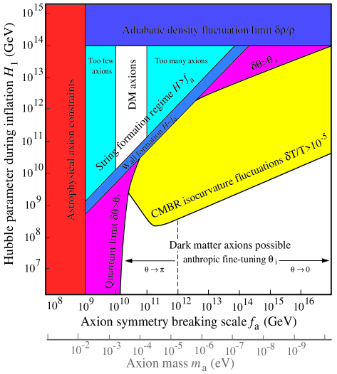
Figure 1: Inflation and the dark matter axion. Constraints on the Hubble parameter $H_{1}$ during inflation and the Peccei-Quinn scale $f_{\rm a}$ and axion mass $m_{\rm a}$. Only the white areas are compatible with a dark matter axion $\Omega_{\rm a}\approx 1$ in simple inflation models. For $H>f_{\rm a}$, the string bound (9) pertains and, for $H<f_{\rm a}$, consistency is due to ‘anthropic fine-tuning’.

Many inflationary models are not very consistent with the requirement (13). For example, the simplest chaotic inflation models have $H_{1}\sim 10^{13}\hbox{--}10^{14}$ GeV, implying a truly invisible axion with $m_{\rm a}\sim 10^{-16}$eV and $f_{\rm a}$ beyond the Planck mass! However, inflation now has many guises and it is possible to engineer models with Hubble parameters anywhere in the range $H\sim 10^{2}\hbox{--}10^{14}$GeV; here, the lower bound is set by supersymmetry considerations and the upper bound by limits on adiabatic density fluctuations (see, for example, ref. [45]). New inflation can have $\!{}^{{\bf?}}$ $H\hbox{${\lower 1.72218pt\hbox{$<$}\atop\raise 0.60275pt\hbox{$\sim$}}$}10^{9}$GeV with a detectable dark matter axion, but the low $H$ accentuates its severe initial condition difficulties $\!{}^{{\bf?}}$ (see recent axion inflation reviews such as ref. [47]). Another way to circumvent the CMB constraint (13) is in more complicated inflationary scenarios in which the Peccei-Quinn scalar field $\phi$ is the inflaton $\!{}^{{\bf?},{\bf?}}$ or else interacts with it, as in a hybrid inflation model. $\!{}^{{\bf?}}$ It is then possible to have $|\phi|>\!>f_{\rm a}$ as the inflaton rolls down to the vacuum, so the quantum fluctuations in (12) will be suppressed  by the factor $f_{\rm a}/|\phi|$. These inflationary caveats and the lack of any definite axion mass prediction has led Linde $\!{}^{{\bf?}}$ to conclude that “the best resolution of the uncertainties would be given by an experimental measurement of the axion mass. … It may also help us to choose between different versions of inflation and axion models.”!

4.2 $H_{1}\hbox{${\lower 1.72218pt\hbox{$>$}\atop\raise 0.60275pt\hbox{$\sim$}}$}f_{\rm a}$: Axion string creation during inflation

Even for a low reheat temperature $T_{\rm reh}<f_{\rm a}$, one can envisage inflation models with a large Hubble parameter during inflation $H_{1}\hbox{${\lower 1.72218pt\hbox{$>$}\atop\raise 0.60275pt\hbox{$\sim$}}$}f_{\rm a}$. The quantum fluctuations (12) in this case are sufficient to take the Peccei-Quinn field $\phi$ over the top of the potential $\!{}^{{\bf?}}$ leaving large spatial variations and non-trivial windings in $\phi$. We can interpret this as the Gibbons-Hawking temperature ‘restoring’ the PQ-symmetry $T_{\rm GH}\hbox{${\lower 1.72218pt\hbox{$>$}\atop\raise 0.60275pt\hbox{$\sim$}}$}f_{\rm a}$. As inflation draws to a close and $H$ falls below $f_{\rm a}$, these fluctuations will become negligible and a string network will form along lines where $\phi=0$. Provided inflation does not continue beyond this point for more than about another 30 e-foldings, we will effectively return to the ‘standard thermal’ scenario in which axions are produced by a decaying string network. It is effectively as if $T_{\rm reh}>f_{\rm a}$, so such low reheat inflation models are compatible with a dark matter axion $\!{}^{{\bf?}}$, $m_{\rm a}\approx 100\mu$eV. This leaves the additional small upper window for the axion shown in fig. 1.

More problematic is the case where $H\sim f_{\rm a}$, or just below, for an extended period, say more than $n>30$ e-foldings. In this case, string formation may be rare, but the field will still be driven around the Mexican hat potential by quantum fluctuations ending up with an average total fluctuation $\delta\theta\sim\sqrt{n}H/2\pi f_{\rm a}\hbox{${\lower 1.72218pt\hbox{$>$}\atop\raise 0.60275pt\hbox{$\sim$}}$}1$. This will imprint non-trivial windings into the axion field which will appear as exponentially large domain walls $\!{}^{{\bf?}}$ when the axion mass ‘switches on’. Depending on their size and distribution these are potentially incompatible with CMB constraints. $\!{}^{{\bf?}}$ A number of other complex hybrid scenarios can arise when $H_{1}\sim f_{\rm a}$, as reviewed in ref. [48].

Up to this point we have only considered the simplest axion models with a unique vacuum $N=1$, so what happens when $N>1$? In this case, any strings present become attached to $N$ domain walls at the QCD-scale. Such a network ‘scales’ rather than annihilates, and so it is cosmologically disastrous. $\!{}^{{\bf?},{\bf?}}$ Consequently, only $f_{\rm a}>H_{1}>T_{\rm reh}$ inflationary scenarios are acceptable for $N>1$ and, for these, constraints like (4) can be suitably adapted by merely rescaling $f_{\rm a}\rightarrow f_{\rm a}/N$.

5 Conclusions

We have endeavoured to provide an overview of axion cosmology focussing on the mass of a dark matter axion. First, the cosmological axion density has been calculated in the standard thermal scenario by considering the dominant contribution from axion strings. In this case there is, in principle, a well-defined calculational method to precisely predict the mass $m_{\rm a}$ of a dark matter axion. For the currently favoured value of the Hubble parameter ($H_{0}\approx 60\rm\,km\,s^{-1}Mpc^{-1}$), the estimate (9) predicts a dark matter axion of mass

$$m_{\rm a}\approx 200\,\mu\hbox{eV}\,,\qquad f_{\rm a}\approx 3\times 10^{10}\hbox{GeV}\,,$$ (14)

where the significant uncertainties from all sources approach an order of magnitude. The key uncertainty in this string calculation is the parameter ratio $\alpha/\kappa$, that is, the ratio of the loop size to radiation backreaction scale. Here, like most authors we have assumed $\alpha/\kappa\approx 1$, however, reducing this uncertainty remains a key research goal, though a technically difficult one.

Secondly, we have reviewed inflationary axion cosmology showing that (i) many inflation models return us to the standard thermal scenario with $m_{\rm a}\sim 100\mu$eV, (ii) some inflation models are essentially incompatible with a dark matter axion and (iii), because of the possibility of ‘anthropic fine-tuning’, other inflation models can be constructed which incorporate a dark matter axion mass anywhere below $m_{\rm a}\hbox{${\lower 1.72218pt\hbox{$<$}\atop\raise 0.60275pt\hbox{$\sim$}}$}1$meV.

We conclude that, while a dark matter axion might possibly lurk anywhere in an enormous mass range below $m_{\rm a}\hbox{${\lower 1.72218pt\hbox{$<$}\atop\raise 0.60275pt\hbox{$\sim$}}$}1$meV, the best-motivated mass for future axion searches lies near $m_{\rm a}\sim 100\mu$eV, a standard thermal scenario prediction which is also compatible with a broad class of inflationary models.

References

References

- [1] R.D. Peccei and H.R. Quinn, Phys. Rev. Lett. 38, 1440 (1977); Phys. Rev. D16, 1791.
- [2] F. Wilczek,, Phys. Rev. Lett. 40, 279 (1978). S. Weinberg, Phys. Rev. Lett. 40, 223 (1978).
- [3] R.L. Davis, Phys. Lett. 180B, 225 (1986).
- [4] R.L. Davis and E.P.S. Shellard, Nucl. Phys. B324, 167 (1989).
- [5] R.A. Battye and E.P.S Shellard, Phys. Rev. Lett. 73, 2954 (1994). Erratum: Phys. Rev. Lett. 76, 2203. R.A. Battye and E.P.S Shellard (1997), Recent Perspectives on Axion Cosmology in Proceedings of Dark Matter in Astro- and Particle Physics, ed. H.V. Klapdor-Kleingrothaus & Y. Ramachers, pp. 554 (World Scientific, 1997), also astro-ph/9706014
- [6] J. Preskill, M.B. Wise and F. Wilczek, Phys. Lett. 120B, 127 (1983). L. Abbott & P. Sikivie, Phys. Lett. 120B, 133 (1983). M. Dine & W. Fischler, Phys. Lett. 120B, 137 (1983).
- [7] G.G. Raffelt (1997), astro-ph/9707268.
- [8] M.S. Turner, Phys. Rep. 197, 67 (1990). G.G. Raffelt, Phys. Rep. 198, 1 (1990).
- [9] C. Hagmann et al (1998), astro-ph/9802061. J.L. Rosenberg, Particle World 4, 3 (1995).
- [10] I. Ogawa, S. Matsuki & K. Yamamoto, Phys. Rev. D53, R1740 (1996).
- [11] A.O. Gattone, et al (1997), astro-ph/9712308. K. Zioutas, et al (1998), astro-ph/9801176. P. Sikivie, D.B. Tanner, & Y. Wang, Phys. Rev. D50, 7410 (1994).
- [12] L.S. Altarev et al., Phys. Lett. 276B, 242 (1992). K.F. Smith et al., Phys. Lett. 234B, 191 (1990).
- [13] J.E. Moody and F. Wilczek, Phys. Rev. D30, 130 (1984).
- [14] J.-E. Kim, Phys. Rep. 150, 1 (1987). J.-E. Kim (1998), astro-ph/9802061.
- [15] D.S.P. Dearbon, D.N Schramm, and G.Steigman, Phys. Rev. Lett. 56, 26 (1986). G.G. Raffelt & D.S.P. Dearborn, Phys. Rev. D36, 2211 (1987).
- [16] A. Vilenkin and A.E. Everrett, Phys. Rev. Lett. 48, 1867 (1982).
- [17] P. Sikivie, Phys. Rev. Lett. 48, 1156 (1982).
- [18] E.P.S. Shellard (1986), in Proceedings of the 26th Liege International Astrophysical Colloquium, The Origin and Early History of the Universe, Demaret, J., ed. (University de Liege). E.P.S. Shellard (1990), ‘Axion strings and domain walls’, in Formation and Evolution of Cosmic Strings, Gibbons, G.W., Hawking, S.W., & Vachaspati, V., eds. (Cambridge University Press).
- [19] M.S. Turner, Phys. Rev. Lett. 21, 2489 (1987).
- [20] M.S. Turner, Phys. Rev. D33, 889 (1986).
- [21] G.G. Raffelt (1998), Mini-Review for the Particle Data Book.
- [22] E.P.S. Shellard & R.A. Battye (1998), ‘Inflationary axion cosmology revisited’, DAMTP preprint.
- [23] A.D. Linde, Phys. Lett. 201B, 437 (1988).
- [24] E. Witten, Phys. Lett. 153B, 243 (1985).
- [25] A. Vilenkin and T. Vachaspati, Phys. Rev. D35, 1138 (1987).
- [26] R.L. Davis and E.P.S. Shellard, Phys. Lett. 214B, 219 (1988).
- [27] A. Dabholkar and J.M. Quashnock, Nucl. Phys. B333, 815 (1990).
- [28] R.A. Battye and E.P.S. Shellard, Phys. Rev. Lett. 75, 4354 (1994). R.A. Battye and E.P.S. Shellard, Phys. Rev. D53, 1811 (1996).
- [29] R.A. Battye and E.P.S. Shellard, Nucl. Phys. B423, 260 (1994).
- [30] D.D. Harari and P. Sikivie, Phys. Lett. 195B, 361 (1987).
- [31] C. Hagmann and P. Sikivie, Nucl. Phys. B363, 247 (1991).
- [32] M. Sakellariadou, Phys. Rev. D44, 3767 (1991).
- [33] A. Vilenkin & E.P.S. Shellard (1994), Cosmic strings and other Topological Defects (Cambridge University Press).
- [34] D.P. Bennett and F.R. Bouchet, Phys. Rev. D41, 2408 (1990).
- [35] B. Allen and E.P.S. Shellard, Phys. Rev. Lett. 64, 119 (1990).
- [36] W.H. Press, D.N. Spergel, & B.S. Ryden, Ap. J. 347, 590 (1989).
- [37] M. Nagasawa, Prog. Theor. Phys. 98, 851 (1997). M. Nagasawa & M. Kawasaki, Phys. Rev. D50, 4821 (1994).
- [38] D.H. Lyth, Phys. Lett. 275B, 279 (1992).
- [39] D.H. Lyth, Phys. Rev. D48, 4523 (1993).
- [40] S.Y-. Pi, Phys. Rev. Lett. 52, 1725 (1984).
- [41] M.S. Turner, F. Wilczek & A. Zee, Phys. Lett. 120B, 127 (1983). A.D. Linde, Phys. Lett. 158B, 375 (1985). D. Seckel & M.S. Turner, Phys. Rev. Lett. 66, 5 (1991). G. Efstathiou & J.R. Bond, MNRAS 218, 103 (1986).
- [42] D.H. Lyth, Phys. Lett. B236, 408 (1990).
- [43] M.S. Turner & F. Wilczek, Phys. Rev. Lett. 66, 5 (1991).
- [44] A.D. Linde, Phys. Lett. 259B, 38 (1991).
- [45] D.H. Lyth (1996), hep-ph/9609431; D.H. Lyth & A. Riotto, in preparation for Physics Reports (1998).
- [46] Q. Shafi & A. Vilenkin, Phys. Rev. Lett. 52, 691 (1984).
- [47] S.D. Burns (1998), astro-ph/9711303.
- [48] D.H. Lyth and E.D. Stewart, Phys. Lett. 283B, 189 (1992). D.H. Lyth and E.D. Stewart, Phys. Rev. D46, 532 (1992).
- [49] A.D. Linde & D.H. Lyth, Phys. Lett. 246B, 353 (1990).