Cosmological Parameters from Multiple-arc Gravitational Lensing Systems I: smooth lensing potentials

Abstract

We describe a new approach for the determination of cosmological parameters using gravitational lensing systems with multiple arcs. We exploit the fact that a given cluster can produce multiple arcs from sources over a broad range in redshift. The coupling between the critical radius of a single arc and the projected mass density of the lensing cluster can be avoided by considering the relative positions of two or more arcs. Cosmological sensitivity appears through the angular size-redshift relation. We present a simple analytic argument for this approach using an axisymmetric, power-law cluster potential. In this case, the relative positions of the arcs can be shown to depend only upon the ratios of the angular-size distances of the source and between the lens and source. Provided that the astrometric precision approaches $\sim$ 0.01 arcsec (e.g. via HST) and the redshifts of the arcs are known, we show that the system can, in principle, provide cosmological information through the angular-size redshift relation.

We next consider simulated data constructed using a more general form for the potential, realistic sources, and an assumed cosmology. We present a method for simultaneously inverting the lens and extracting the cosmological parameters. The input data required are the image and measured redshifts for the arcs. The technique relies upon the conservation of surface brightness in gravitationally lensed systems. We find that for a simple lens model our approach can recover the cosmological parameters assumed in the construction of the simulated images.

1 Introduction

One particularly promising approach for measuring the large-scale geometry of the universe is through the exploitation of gravitational lensing of distant galaxies and quasars. For some time gravitational lensing has been examined as a possible means of constraining cosmological parameters such as $q_{0}$ and $\lambda$. (e.g.  Turner, 1990) To date most methods have focused on statistical arguments based on the cross sections for strong lensing of background objects (e.g.  Cen et al., 1994). As an alternative we are investigating the feasibility of a method which makes more direct use of the dependence of gravitational lensing events on the geometry of the spacetime between the observer, the source and the lens. The method is motivated by recent images of cluster systems containing numerous arcs (e.g.  Luppino et al., 1994; Kneib et al., 1996). The method works by requiring consistency between both a single mass model for the cluster and a single angular-size redshift relation for all the lensed sources.

We begin with an overview of gravitational lensing, followed by an analytic argument assuming an axisymmetric potential for the lensing cluster given by a power-law in density. We show that the astrometric precision afforded by HST is sufficient to distinguish between differing cosmologies through the angular-size redshift relation. We then investigate more realistic models for the lensing cluster and sources. However, in these cases the resulting arcs have more complicated morphology such that the lens and the geometry must be inverted via ray tracing and the minimization of a suitable merit function (e.g. one based upon the conservation of surface brightness and reasonable morphology of the sources, etc.) Kochanek et al. (1989). In section 3 we present an analysis of simulated data generated with an assumed form for the lensing potential and an arbitrary cosmology. With the simulated image and the redshifts of the arcs as input data we find that we can recover both the parameters describing the lensing mass distribution and the cosmology. In section 4 we discuss the results of this analysis. We develop estimates of the bounds that could be set on cosmological parameters from a hypothetical system with the characteristics of our simulation, and we argue that this technique is a good complement to existing methods for the determination of cosmological parameters because it is purely geometrical rather than statistical in nature and is insensitive to evolutionary effects. In the concluding section we summarize the results of the previous sections, and we describe further refinements to our analysis which will be detailed in subsequent papers in this series.

2 Gravitational Lensing of Multiple Sources

Gravitational lensing is sensitive to the gravitational potential of the lens, the angular position of the source object relative to the lens, and the angular size distances between observer, lens, and source (fig. 1). This last is of principal interest, since the dependence of angular size distance on redshift has a direct dependence on cosmological parameters (e.g.  Sandage, 1988). Large arcs are produced by the near alignment of distant sources (i.e. galaxies) and an intervening cluster of galaxies Paczynski (1987); Soucail et al. (1987); Lynds & Petrosian (1989). For an axisymmetric (thin) lens with an on-axis source, the “critical radius” at which the source is observed depends only upon the projected surface mass density and the angular size distances to the lens and the source Blandford & Narayan (1992). Thus, by measuring redshifts for the gravitationally lensed sources and explicitly including the cosmological dependence of angular size distance on those redshifts, constraints could be set upon various cosmological models. We believe that the recently observed cluster systems with several multiply imaged arcs offer one of the best opportunities for obtaining meaningful constraints. We exploit the fact that sources distributed over a range in redshift can be imaged by the same lens. This should allow us to separate the effects of the lens mass distribution from the cosmological effects.

The technique we propose involves inverting the lens system using methods similar to those presented in Kochanek et al. (1989), but with one important difference; multiple sources at different redshifts are included. Inclusion of multiple source planes admits the possibility of cosmological dependence (q.v. §§ 2.1,3.1), which is treated in our models by including the cosmological parameters as additional fitting parameters. For each cosmological model being tested the distances to all of the sources are computed using the redshifts and the particular cosmological model under consideration. The distances so calculated affect the quality of the fit, and this gives our method its cosmological sensitivity. While this does increase the number of free parameters in our model, we will show that the existence of multiple multiply imaged sources allows the modeled distances to be recovered with sufficient accuracy to provide interesting constraints on cosmological parameters.

2.1 Analytic Treatment of an Axisymmetric System

We can gain an understanding of the cosmological sensitivity of multiple-arc gravitational lens systems by considering a simple, if somewhat contrived, analytically treatable model. Accordingly, consider a cluster potential approximated as an axisymmetric power law in density.

$$\rho(r)=\rho_{a}\left(\frac{a}{r}\right)^{b}.$$ (1)

The projected mass density is then

$$\Sigma_{M}(R)=\rho_{a}a^{b}{\cal I}R^{1-b},$$ (2)

where

$${\cal I}\equiv\int_{-\frac{\pi}{2}}^{\frac{\pi}{2}}d\theta cos^{b-2}\theta,$$ (3)

which is independent of $R$. Integrating equation (2) gives the total projected mass within the projected radius, $R$.

$$M(R)=2\pi\rho_{a}a^{b}\frac{{\cal I}}{3-b}R^{3-b}.$$ (4)

For $b=2$ this equation reduces to the familiar isothermal case (c.f. Breimer & Sanders, 1992).

For simplicity, consider the case of on-axis sources, which would appear as “Einstein Rings” at the angular critical radii, $\theta_{E}$. Then

$$\theta_{E}^{2}=\frac{4G_{N}M(\theta_{E})}{c^{2}}\frac{D_{ls}}{D_{l}D_{s}},$$ (5)

where $D_{l}$, $D_{s}$, and $D_{ls}$ are the angular size distances of the lens, source, and lens-to-source, respectively (c.f. Schneider, Ehlers, & Falco, 1992, §2.1). Since $R\equiv D_{l}\theta$ we can combine equations (4) and (5) such that:

$$\theta_{E}^{2}=\frac{8\pi G_{N}}{c^{2}}\rho_{a}a^{b}\frac{{\cal I}}{3-b}D_{l}^{2-b}\frac{D_{ls}}{D_{s}}\theta_{E}^{3-b},$$ (6)

whence

$$\theta_{E}=\left(\frac{8\pi G_{N}}{c^{2}}\rho_{a}a^{b}\frac{{\cal I}}{3-b}D_{l}^{2-b}\right)^{\frac{1}{b-1}}\left(\frac{D_{ls}}{D_{s}}\right)^{\frac{1}{b-1}}.$$ (7)

Thus, the angular radius of a given arc depends upon both the characteristics of the lens object and the angular-size distances to the source and lens-to-source. Note that for a particular lens system with multiple sources at differing distances the first expression on the left hand side of equation (7) is fixed, and only the second varies between sources.

Now consider the case of multiple arcs. The ratio of the Einstein radii for two sources, $k$ and $m$ is

$$\frac{\theta_{k}}{\theta_{m}}=\left(\frac{D_{ls}^{(k)}}{D_{s}^{(k)}}\right)^{\frac{1}{b-1}}\left(\frac{D_{s}^{(m)}}{D_{ls}^{(m)}}\right)^{\frac{1}{b-1}}.$$ (8)

We can combine this relation for three arcs, $k,m,\text{and}\ n$ to eliminate $b$.

$$\frac{\ln\left(\frac{\theta_{k}}{\theta_{m}}\right)}{\ln\left(\frac{\theta_{k}}{\theta_{n}}\right)}=\frac{\ln\left(\frac{D_{ls}^{(k)}D_{s}^{(m)}}{D_{s}^{(k)}D_{ls}^{(m)}}\right)}{\ln\left(\frac{D_{ls}^{(k)}D_{s}^{(n)}}{D_{s}^{(k)}D_{ls}^{(n)}}\right)}.$$ (9)

The left side of equation (9) is an observational quantity which can in principle be measured directly, and the right side is a cosmological factor which can be calculated for any desired cosmological model, given the redshifts of the arcs. Thus, the relative radii of giant arcs has cosmological sensitivity and can provide a direct test of cosmological models.

Standard error propagation techniques can be applied to equation (9) to determine the astrometric precision required to allow sensitivity to cosmological effects. Let the angular radii, $\theta$ of the arcs be measurable with errors of $\pm\sigma$. Then the error in

$${\cal R}\equiv\frac{\ln\left(\frac{\theta_{k}}{\theta_{m}}\right)}{\ln\left(\frac{\theta_{k}}{\theta_{n}}\right)}$$ (10)

is given by

$$\sigma_{\cal R}^{2}=\frac{\sigma^{2}}{\left(\ln\left(\frac{\theta_{k}}{\theta_{n}}\right)\right)^{2}}\left[\frac{1}{\theta_{k}^{2}}-\frac{1}{\theta_{m}^{2}}-\left(\frac{\ln\left(\frac{\theta_{k}}{\theta_{m}}\right)}{\ln\left(\frac{\theta_{k}}{\theta_{n}}\right)}\right)^{2}\left(\frac{1}{\theta_{k}^{2}}-\frac{1}{\theta_{n}^{2}}\right)\right].$$ (11)

We can evaluate equation (11) for a typical lens system, assuming a standard $\Omega=1$, $\lambda=0$ cosmology. Consider a lens system ($z_{l}=0.4$) with three arcs ($z_{1,2,3}=0.6,0.8,1.2$). For $\theta(z\rightarrow\infty)=30\arcsec$ the system produces arcs with angular radii $\theta_{1,2,3}=7\farcs 8,11\farcs 8,15\farcs 7$. These values in equation (11) yield the result

$$\sigma_{\cal R}\approx 0.1\sigma\text{(arcsec)}.$$ (12)

The right hand side of equation (9) can be evaluated for any desired cosmology. Figure 2 shows calculated values of ${\cal R}$ for two families of cosmological models: flat cosmologies and $\lambda=0$ cosmologies. From these we can conclude that a measurement error of $\sigma_{\cal R}\approx 0.001$ would allow marginal discrimination between extreme cosmological cases. This corresponds to a measurement error in the positions of the arcs of $\sigma_{\text{arc}}\approx 0\farcs 01$.

We can compare the results of this section to the astrometric precision one might expect to obtain from presently available instruments. Examination of arcs imaged by HST shows that the cross section of a representative arc has a FWHM of $0\farcs 2$. The arcs have a typical signal-to-noise ratio of 10. A simple monte carlo calculation indicates that the positions of the arcs should be measurable to an error of $\sigma_{\text{arc}}\approx 0\farcs 02$. Such a measurement would result in marginal discrimination between cosmological models (fig. 2).

Real gravitational lens systems are expected to be more complex than these analytically soluble systems. Moreover, even for the simple potentials we have discussed, the off-axis sources present in real systems introduce an additional error term which can dominate the contribution to the total error. Consequently, the technique of comparing the astrometric positions of the observed arcs to their calculated positions for the models being tested is ill-suited for application to real systems. In section 3 we describe a numerical technique which addresses both of these issues.

3 Evaluation of More Realistic Cases Using Simulated Data

The surface brightness of a bundle of light rays is unchanged by gravitational deflection Blandford & Narayan (1992). We can exploit this property to construct a technique for analyzing systems more realistic than that described in section 2.1. With this method comparing the surface brightnesses of image pixels mapped to the same point in the source plane replaces the measurement of arc positions as our primary test of the quality of a model.

3.1 Lensing Potential

The lensing potential is defined by

$$\boldsymbol{\alpha}(\boldsymbol{\theta})=\boldsymbol{\nabla}\psi(\boldsymbol{\theta}),$$ (13)

where $\boldsymbol{\alpha}$ is the reduced deflection angle depicted in figure 1, and $\boldsymbol{\theta}$ is the position angle at which the source is observed. Thus, we see that the lens mapping is defined by

$$\begin{split}\boldsymbol{\beta}&=\boldsymbol{\theta}-\boldsymbol{\alpha}\\ &=\boldsymbol{\theta}-\boldsymbol{\nabla}\psi(\boldsymbol{\theta}).\end{split}$$ (14)

We adopt an elliptical lensing potential of the form (e.g.  Blandford & Kochanek, 1987)

$$\psi(x,y)=\frac{(b^{2})^{1-q}}{2q}(s^{2}+(1+\epsilon_{c})x^{2}+2\epsilon_{s}xy+(1-\epsilon_{c})y^{2})^{q}.$$ (15)

In this expression $b$ is the angular critical radius (i.e. the radius of the critical curve), measured in arc-seconds, for an axisymmetric ($\epsilon_{c}=\epsilon_{s}=0$) lens, $s$ is the angular core radius, $q$ is a function of the power-law index of the mass density distribution ($0\leq q\leq 0.5$), and $\epsilon_{c}$ and $\epsilon_{s}$ are related to position angle, $\phi$, of the major axis and the ellipticity, $\epsilon$, of the potential by:

$$\epsilon_{c} =\epsilon\cos(2\phi);$$ (16)

$$\epsilon_{s} =\epsilon\sin(2\phi).$$ (17)

It is worth noting that this form for the potential suffers from several defects. First, it retains the same ellipticity out to arbitrary distances; this is in contrast to the expected axisymmetric behavior at large distances from a mass distribution of finite extent. A related problem is that the surface mass density distributions produced by such a potential are unrealistic (“peanut-shaped”) or unphysical (negative) at large radii. However, for sufficiently small $\epsilon$ (Blandford & Kochanek (1987) suggest $\epsilon<0.2$) these anomalies occur at large enough radii that they do not affect the lensing behavior within the region of interest. While alternative potentials based on elliptical mass distributions have been studied, their lensing behavior is qualitatively the same within the region of interest as the elliptical potentials Kassiola & Kovner (1993). Consequently, we adopt the simpler potentials for this study.

A potential of the form given in equation (15) is sufficient to describe a system with a single source. However, for the case of multiple sources at differing redshifts lensed by the same mass distribution, $b$ is different for each source. The constraint that each source is being lensed by the same mass distribution can be incorporated into a lensing potential of the form:

$$\psi(x,y)=\zeta_{k}\frac{(b^{2})^{1-q}}{2q}(s^{2}+(1+\epsilon_{c})x^{2}+2\epsilon_{s}xy+(1-\epsilon_{c})y^{2})^{q},$$ (18)

where $b$ is now the same for each source and is equivalent to the critical radius as $z\rightarrow\infty$. For the $k$th source $\zeta_{k}$ is given by

$$\zeta_{k}=\frac{D_{ls}^{(k)}}{D_{s}^{(k)}}.$$ (19)

With this form for the lensing potential the critical radius for each source is

$$b_{k}=\zeta_{k}^{\frac{1}{2-2q}}b.$$ (20)

Since the angular size distances $D_{ls}^{(k)}$ and $D_{s}^{(k)}$ are functions of $\Omega$ and $\lambda$ equation (18) allows us to include the cosmological parameters as fitting parameters in our model, with the distances recalculated each time the cosmological portion of the model is varied.

3.2 Simulation of input data

Our inversion requires two forms of input data: the redshifts of the lens and arcs and a high-resolution image of the system. In order to test the algorithm, simulated data sets were constructed using the following procedure. First a set of model parameters was selected. These parameters include the adjustable lens parameters in equation (18), the cosmological parameters, $\Omega$ and $\lambda$, the number of sources to be used, and the redshifts of the sources. The lens parameters were chosen to be representative of clusters of galaxies. The parameters used in our simulation are summarized in Table 1. Source positions were arbitrarily selected but chosen such that strongly lensed arcs are produced. Realistic sources were constructed using a representative galaxy extracted from the Hubble Deep Field (Williams et al., 1996, hereafter HDF). The redshifts for the lens and the four sources were chosen to be 0.2, 0.4, 0.6, 0.75, and 1.25, respectively.

To incorporate HDF sources, several galaxies from the field were selected and tested; however, the models produced seemed to differ little, provided that the sources selected were scaled to a size appropriate for typical gravitational lensing sources. Ultimately, a single source was selected as being representative of the field and used for all of the sources in our simulations. Since the redshifts of most of the HDF sources are unknown, we scaled our source galaxy to produce simulated arcs of similar width to actual arcs. The background and peak intensities of these sources were also scaled in order to produce a desired signal-to-noise ratio in the arcs.

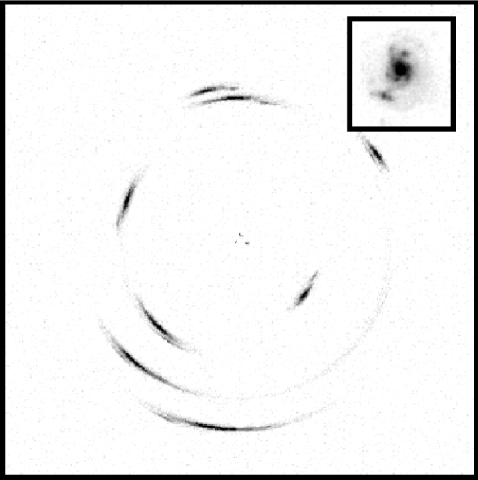
Figure 3: The simulated image used in this study. The inset shows a source extracted from the Hubble Deep Field and used to construct the simulated data. The source was scaled and resampled to produce sources at each redshift in the simulated system.

Once model parameters are selected, each pixel in the image plane is mapped, via the lens mapping equation (14), into each source plane using the angular-size redshift relation. Several methods were considered for selecting the appropriate surface brightness in the presence of several source planes, including the maximum brightness in any of the source pixels, the sum of the brightnesses of the source pixels, and the first (lowest redshift) source pixel encountered with a brightness above a particular threshold. In practice, since an image pixel does not generally map to bright regions in more than one source plane, there was little difference between the methods. Therefore, the surface brightness assigned to the image pixel is the maximum of the surface brightnesses of the source pixels to which it is mapped in each of the source planes. To produce a desired signal-to-noise ratio in the image a constant background level is added to each image pixel, and noise in the form of random Poisson deviates is added to the simulated image. The image produced by this simulation is shown in figure 3 (plate 00).

The image produced by the simulation is stored for use as input to our inversion method. Also, the bright pixels in the image (i.e. the arcs) are identified with the source plane which produced them (i.e. the process fills the role of measuring the redshifts of real arcs). These data, along with the redshifts of the source planes, form the input data for the inversion method. The model parameters used in the simulation are stored for comparison to the results of inversion attempts, but are not otherwise used.

3.3 Merit function for inversion procedure

A numerical model under consideration is evaluated by computing a merit function, $f$, for the model and comparing it to the merit functions of other models. Ideally, the merit function is so constructed that it has a unique minimum at the “true” solution.

Kochanek et al. (1989) proposed a merit function based on the fact that surface brightness is conserved in gravitational lensing. We adopt a similar merit function, but with a few modifications which we find result in more robust behavior for our multi-source models. Our merit function is given by

$$f=\bar{e}+w_{O}O+w_{S}S.$$ (21)

In equation (21) $\bar{e}$, $O$ and $S$ are functions defined below which measure the properties that differentiate “good” models from “bad”. Specifically $\bar{e}$ measures the degree to which surface brightness is preserved in the lens mapping; $O$ measures the degree to which the input image data is reproduced by that reconstructed from the model under consideration; and $S$ measures the degree of fragmentation in the reconstructed sources (i.e. sources should resemble galaxies.)

The quantities $w_{O}$ and $w_{S}$ are weights which ensure that the quantities being summed are all roughly of the same order of magnitude For the models presented here the weights used were

$$w_{O} =5,$$

$$w_{S} =0.005.$$

The ‘penalty’ functions, $O$ and $S$ are designed to enforce physical constraints upon the numerical minimization algorithm. In practice the weight coefficients can be set to zero once the algorithm nears a solution.

The components of the merit function are calculated as follows; an image of the system and measurements of the redshifts of the arcs visible in the system are required as input data. Arcs are identified as regions with a surface brightnesses above a particular “arc-threshold.” The image plane is divided into regions corresponding to objects of measured redshift, blank regions, and regions containing blocking foreground or cluster objects. At present we assume that redshifts can be measured for each arc in the system. This allows each arc to be identified with a particular source plane. Given a set of model parameters to be evaluated sources are reconstructed by ray tracing the image pixels back into the source planes corresponding to the appropriate redshifts. Each source pixel is then assigned the average of the values of the image pixels mapped to that source pixel. Additionally, multiply imaged pixels in each source plane are identified. Background pixels are not used in the reconstruction of the sources owing to the fact that they have no measured redshifts, and hence cannot be identified with a particular source plane. However, they are used in comparing the input and reconstructed images as described below.

The function $\bar{e}$ measures the preservation of surface brightness and is defined by

$$\bar{e}=\sum_{i,j,k}\frac{1}{\sigma^{2}_{ij}(n_{ijk}-1)}\sum_{m=1}^{n_{ijk}}(I^{m}_{ijk}-S_{ijk})^{2}.$$ (22)

Here, $k$ is summed over the source planes, and $i$ and $j$ are summed only over the multiply imaged pixels in each plane. $S_{ijk}$ is the value of the source pixel, $n_{ijk}$ is the multiplicity with which it is imaged, $I^{m}_{ijk}$ is the value of the $m$th image pixel identified with the source pixel, and $\sigma_{ij}$ is the noise in the pixel.

In order to measure how well the image is reproduced, a reconstructed image is made from the source planes and the model parameters being evaluated. The function $O$ is defined by

$$O=\frac{1}{N}\sum_{i,j}|I_{ij}-R_{ij}|,$$ (23)

where $I_{ij}$ refers to the surface brightness of pixel $i,j$ of the input image, $R_{ij}$ refers to the surface brightness of the same pixel in the reconstructed image, and $N$ refers to the total number of pixels in the image. Since the sources are constructed to reproduce the observed arcs, the principal contribution to $O$ is from pixels which were background in the input image, but which are brighter than the arc-threshold in the reconstruction. For real data, regions of the image for which there is no information (e.g. a blocking foreground object or non-transparent portion of the lens) would be excluded from the calculation of $O$. The sum is in practice limited to those pixels whose brightness exceeds the arc-threshold in the reconstructed image in order to prevent Poisson fluctuations in the background from dominating $O$.

The morphology of galaxies at high redshift is not well known; however, we expect the surface brightness of neighboring pixels in a source plane to be correlated. Thus, we include a contribution to the merit function which measures the deviation of neighboring pixels in the source plane. The function $S$ is defined by

$$S=\sum_{i,j,k}\frac{1}{8}\sum_{m,n=i,j\pm 1}|S_{ijk}-S_{mnk}|,$$ (24)

where the subscripted $S$ refers to pixel values in the various source planes. Mathematically, $S$ is the average difference between a pixel and its eight neighbors in the same source plane. This statistic measures the degree to which the source object is fragmented in the source plane; a contiguous source (e.g. one resembling a galaxy) is preferred over a fragmented source (e.g. one resembling a demagnified version of the arcs in the image).

3.4 Determination of Model Parameters

In order to extract the best fitting model parameters from the system, we must find the minimum of the merit function over nine parameters. Unfortunately, we were not able to design an automatic, globally convergent procedure for finding this minimum. The principal obstacle to creating such a procedure is that the merit function surface has much larger gradients in some principal directions than in others. Furthermore, far from the solution the merit function surface levels off to form a plateau with no large-scale gradient to indicate to an algorithm which way the minimum lies. The first problem can be overcome by making use of the underlying physical relationships among the parameters. The second problem can be addressed by noting that for each of the parameters there is an empirically determined “characteristic scale” within which an automatic minimization algorithm is convergent. Low-resolution scans can be made of the parameter space such that suitable initial starting values can be chosen. The characteristic scales for the model parameters were determined from an extensive search of the parameter space and are given in Table 1.

3.4.1 Computational Techniques

To fully exploit the information contained within HST images of arc systems requires the use of a high-resolution grid of image and source pixels. The many evaluations of the merit function in a minimization algorithm places large demands on computer resources. The work presented here was performed using the SCAAMP collaboration’s 64-processor Silicon Graphics Origin 2000. The facility has maximum throughput of 21 Gflops, although our calculations typically used only 16 of the 64 processors. The availability of this resource allowed us to thoroughly study the parameter space in a reasonable amount of time. Details regarding the software developed for this procedure will be presented at a later date Link (1998).

A high-resolution scan of the parameter space was performed in order to determine the characteristic scales of the model parameters (Table 1). We believe these scales will be generally applicable to gravitational lens systems parameterized in the form of equation (18). Since the characteristic scales determine the size of the neighborhood of convergence, a scan of parameter space at this resolution can be used to select initial guesses for a minimization algorithm. Some representative slices of the parameter space are shown in figure 4.

Having selected initial guesses we fix the cosmological parameters at reasonable values, the remaining parameters are determined using a standard downhill simplex technique Press et al. (1988). Since the cosmological parameters have a small, second-order effect on the model we find that it is possible to arrive at a good solution for the lens parameters regardless of the initial guesses for cosmological parameters.

Once the mass parameters for the system are obtained we solve for the cosmological parameters. Although small, the cosmological effects are strongly coupled only to the effects of the $b$ parameter (c.f. equation 18.) Thus, with the exception of $b$, the lens mass parameters are held constant while the cosmological parameters are being varied.

The correlation between $b$ and the cosmological parameters can be understood as a tradeoff between the terms multiplying the front of the right side of equation (18). This relationship can be used to assist the minimization algorithm in finding the cosmological solution once the mass parameters have been found. To further understand this relation, consider a simple system with only one source. Let us, however, describe this system using the form of the lensing potential given in equation (18). Then, all other things being equal, models for which

$$\frac{D_{ls}}{D_{s}}b^{2(1-q)}=\text{constant}$$ (25)

will produce identical arc systems. In the case of multiple source models we find that the minimal surface can be approximated by

$$\zeta b^{2(1-q)}=\Upsilon$$ (26)

where $\Upsilon$ is a constant, and $\zeta$ represents the distance ratio, $D_{ls}/D_{s}$ for some sort of “characteristic” redshift of the sources. We find that by taking this characteristic redshift to be the median redshift of all of the sources, a reasonable approximation of the relationship between $b$ and $\Omega$ (with other parameters constant) can be obtained in the neighborhood of the solution. However, since this approximation is strictly true only for the median redshift, we use equation (26) only to provide an initial guess for a one-dimensional minimization in $b$ at each evaluation of the merit function.

4 Results

We find that the minimization procedure outlined in the previous section converges to the global minimum of the merit function if the initial guesses for the model parameters are within a “neighborhood of convergence” about the correct values. This neighborhood is readily identifiable from the low-resolution parameter space scans described in section 3.4. For a signal-to-noise ratio of 10 in the simulated data the lens parameters recovered by the algorithm are essentially indistinguishable from their fiducial values (q.v. Table 1), while the cosmological parameters recovered are accurate to within $\sim$10%.

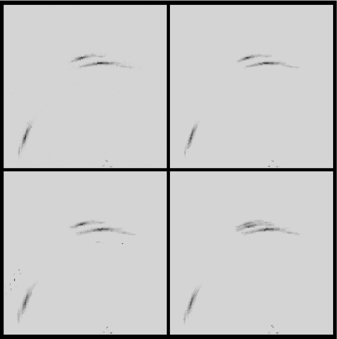
Figure 5: A comparison of a fixed region within (clockwise from upper-left) the simulated image, the image reconstructed from the best fit model (see also Table 1), and the images reconstructed from the best fit models with cosmological parameters fixed at $\Omega=0$, $\lambda=1$, and $\Omega=0.2$, $\lambda=0$, respectively. Note that the best fit model reproduces the simulated image well, while the others have noticeable defects.

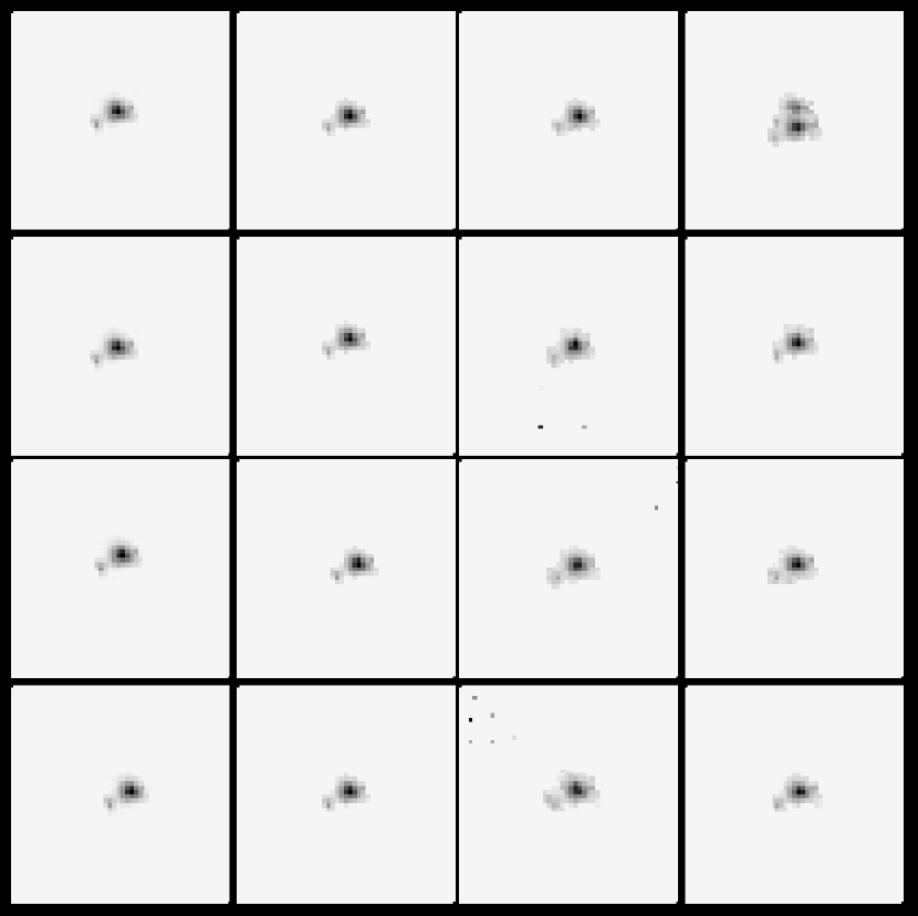
Figure 6: A comparison of the input data and reconstructed source planes for the models shown in figure 5. From top to bottom are the four source planes corresponding to the redshifts of the arcs in the system. From left to right are the input data, the best fit model, and the best fit models with $\Omega=0$, $\lambda=1$ and $\Omega=0.2$, $\lambda=0$. Note that as was the case for the reconstructed images, the best fit model reproduces the simulated data well, while there are noticeable defects in the sources corresponding to the other models, particularly at the two redshift extremes.

We can gain some insight into the cosmological sensitivity of our technique by examining the morphology of sources and images reconstructed from a selection of cosmological models. In figures 5 and 6 (plates 00,00) we compare the simulated data with that reconstructed from both the best fit model and models with the cosmological parameters fixed at $\Omega=0$, $\lambda=1$ and $\Omega=0.2$, $\lambda=0$. In each of the latter two cases the non-cosmological parameters were varied in order to produce the best fit model for the cosmological model under consideration. Figure 5 shows a portion of the simulated image and corresponding regions of the image reconstructed from the model recovered by the algorithm and of images reconstructed from models with the cosmological parameters fixed at $\Omega=0$, $\lambda=1$ and $\Omega=0.2$, $\lambda=0$. Figure 6 shows the four source planes corresponding to each of these images. While the images and sources for the incorrect cosmological models are similar to the originals, they contain noticeable defects. In contrast, the reconstructions from the model arrived at by the minimization algorithm appear substantially better.

Figure 7 shows contours of the merit function involving the cosmological parameters. Note that the cosmological parameters show strong correlations with $b$. This is due to the fact that these parameters affect the overall scale of the system through the $\zeta_{k}$ in equation (18). Hence, for the first three panels $b$ was adjusted to produce the minimal value of $f$ at each point in the contour. This allows us to isolate the intrinsic effects of the cosmological parameters from those that result from changing the overall multiplicative constant in the lensing potential.

Of particular interest is the slice in $\Omega$ and $\lambda$, since this characterizes our cosmological sensitivity. For our particular simulation the cosmological sensitivity is primarily to $\Omega$ rather than $\lambda$. This is partly a result of the fiducial model we have chosen for this study and partly a consequence of the range of redshifts chosen for the simulation. By choosing $\Omega=1$, $\lambda=0$, a strongly mass-dominated model, for our fiducial cosmology, we effectively mask the influence of $\lambda$ unless $\lambda$ is comparable to $\Omega$. Moreover, the angular size-redshift relation, upon which this technique depends for its cosmological sensitivity, is sampled only over the range redshifts of spanned by lens and the sources. Consequently, cosmological models which produce similar angular size-redshift relations over those redshifts will “look” similar. Examination of equation (18) reveals that the cosmological parameters enter into the lensing potential through the leading multiplicative term:

$$\xi=\frac{b^{2(1-q)}}{2q}\zeta(z)$$ (27)

Figure 8 illustrates the dependence of this expression on redshift for selected cosmological models. For each cosmological model we evaluate the quantity $\xi$ in equation (27), using the values of $b$ and $q$ which minimize $f$, and compare this to the same quantity evaluated for the fiducial cosmology. The differences are plotted as a function of redshift for each cosmological model. For comparison we show three cosmological models of interest: model I, a flat, low-omega model; model II, a $\lambda=0$, low-omega model; and model III, a model along the near-minimal surface of $f$ in the $\Omega$-$\lambda$ plane. Note that the residuals for model III are substantially smaller than those for the other models over the range of redshifts represented in the simulated data. Thus, it is understandable that model III is a better fit (as measured by its relatively low value of $f$) than models I and II. Therefore, the shape of the merit function contours in the $\Omega$–$\lambda$ plane results from the behavior of equation (27) over the range of redshifts sampled by the lens and sources. Specifically, the contours are elongated in the direction of cosmological models that produce values of $\xi$ similar to those of the fiducial model at the sampled redshifts.

4.1 Monte carlo estimate of confidence regions

We have identified four principal sources of error in the parameters determined using our method. These are: the noise in the input image, errors in the redshift measurements, deviation of the actual lens potential from our parameterized form, and any density fluctuations along the line of sight which alter the angular size-redshift relation. We consider only the first two sources of error in this study; although the others will be addressed in subsequent papers in this series.

In order to evaluate these first two sources of error, we have performed monte carlo calculations to estimate confidence regions in the cosmological parameters. At each iteration of these calculations new simulated data are constructed from the fiducial model described in the previous sections, using a new seed to create an independent image of the system with the same signal-to-noise ratio as the original. Next, errors with a Gaussian distribution are added to the redshifts in the model, and the merit function, $f$, is calculated for the fiducial parameters and the perturbed redshifts. The process is repeated until a sufficiently large sample is collected; in this case 100 samples were used. The contour in the $\Omega$–$\lambda$ parameter space corresponding to the 68.5 percentile of $f$ is adopted as an estimate for the $1\sigma$ confidence region for $\Omega$ and $\lambda$. Figure 9 shows the $1\sigma$ confidence regions obtained through this technique for several values of $\sigma_{z}$, the standard error in the redshifts. With a peak signal-to-noise ratio of ten in the image arcs, the contribution from the measurement errors in the redshifts is by far the dominant effect.

If we adopt $\sigma_{z}=0.001$ as a typical error in current measurements the allowed region of the $\Omega$–$\lambda$ parameter extends over a broad range in $\lambda$ and a modest range in $\Omega$. However, much of the parameter space is nevertheless excluded. In particular, our method strongly strongly discriminates between “interesting” cosmological models, viz. flat cosmologies ($\Omega+\lambda=1$) and $\lambda=0$ cosmologies. For these classes of models the constraints from this approach are strong. Results for these specific cases are summarized in Table 2. It is worth noting that the allowed range of cosmological parameters is significantly reduced if the error in the arc redshifts can be reduced to $\sigma_{z}\approx 0.005$. While such measurements are difficult, they are not beyond the reach of 10-m class telescopes.

5 Concluding Remarks

Our inversion technique is able to extract both the lens and the cosmological parameters used to construct the simulated data. Moreover, the confidence regions obtained in our monte carlo calculation suggest that physically interesting constraints could be set on cosmological parameters through this method. The requisite data, high-resolution images from HST and redshifts for the arcs, are are currently obtainable. We are encouraged by recent observations which include systems with multiple sources Luppino et al. (1994); Kneib et al. (1996), and by the fact that some systems appear to have sources at several redshifts Hogg et al. (1996).

We have made several simplifying assumptions in our analysis, particularly the use of the same analytic potential for both simulating and analyzing the data. We are currently engaged in further work studying the cosmological constraints which result from applying this technique to a potential whose form is not known a priori, and which may contain substructure. Presumably these factors will introduce additional error which may weaken the constraints which can be set on cosmological parameters using this technique. However, in view of the success we have experienced with our simulations to date we believe that the errors so introduced will be surmountable and that this method is capable of placing interesting bounds on cosmological parameters.

Figure 1: The geometry of gravitational lensing in the thin lens approximation. For a light ray passing through the lens plane at impact parameter $\xi$, the reduced deflection angle ($\alpha$) is given by the gradient of the lensing potential. The undeflected position of the source ($\beta$) is related to the observed position ($\theta$) by the lens mapping (equation 14 in text). All distances are angular size distances.

Figure 2: The dependence of relative angular radii of gravitational arcs on cosmological parameters for an analytically soluble axisymmetric lens model (see § 2.1). Here ${\cal R}=\ln\left(\frac{\theta_{1}}{\theta_{2}}\right)/\ln\left(\frac{\theta_{1}}{\theta_{3}}\right)$. Computed values of ${\cal R}$ are shown for two families of cosmological models. For comparison the we include a conservative estimate of the uncertainty for measurements obtainable using HST.

Figure 4: Contours of the merit function, $f$, for a selection of 2-D slices in the parameter space. In each case the cross marks the fiducial parameters used in the simulation. Note the correlation between the power-law index of the lens potential, $q$, and the overall scale factor, $b$ (q.v. equation 18).

Figure 7: Contours of the merit function, $f$, for parameter space slices including the cosmological parameters ($\Omega$ and $\lambda$). In slices not involving $b$, we adopt the value of $b$ which minimizes $f$ with other parameters fixed. In each case the cross marks the parameters used in the simulation. Note in panel (d) the correlation between $b$ and $\Omega$ which results from the fact that both parameters affect the overall scale of the system. Note also the existence of a well-defined minimum in the cosmological parameters. This demonstrates the ability of this technique to discriminate between cosmological models.

Figure 8: Residuals of the quantity $\xi$ in equation 27 with respect to the fiducial model as a function of redshift. The crosses mark the redshifts of the arcs in our simulated data. Models which produce small residuals at these redshifts should produce “better” fits with this technique. Model I is a flat, low-omega model, model II is a $\lambda=0$, low-omega model, and Model III is a model along the curve of the elongated contours of $f$ in the $\Omega$–$\lambda$ plane (figures 7 and 9). Note that model III, which produces the best fit of these three, also produces the smallest residuals of $\xi$ with respect to the fiducial model.

Figure 9: A contour of the merit function, $f$, in the $\Omega$–$\lambda$ subspace showing the confidence region estimated for several values of $\sigma_{z}$ using the procedure in section 4.1. For $\sigma_{z}=0$ (i.e. no measurement errors in the redshifts of the arcs) the estimated confidence region is approximately the size of the cross which marks the fiducial model. Although the allowed region is fairly large with typical redshift errors, along the directions of astronomical interest ($\Omega+\lambda=1$, shown by the dashed line, and $\lambda=0$) the constraints are quite strong (q.v. Table 2).

Table 1: Simulation Parameters

Parameter	Characteristic Length	Fiducial Value
$\Omega$	large	1.0
$\lambda$	large	0.0
$b$	1$\farcs$5	15$\farcs$0
$q$	0.05	0.45
$s$	1″	2$\farcs$5
$\epsilon_{c}$	0.05	0.025
$\epsilon_{s}$	0.05	0.025
$x_{0}$	1″	0$\farcs$0
$y_{0}$	1″	0$\farcs$0

Table 2: Cosmological Bounds vs. Redshift Errors.

Case	$\sigma_{z}=0.001$	$\sigma_{z}=0.0005$
$\Omega+\lambda=1$	$\Omega>0.8$, $\lambda<0.2$	$\Omega>0.9$, $\lambda<0.1$
$\lambda=0$	$0.8<\Omega<1.2$	$0.9<\Omega<1.1$
$\Omega=1$	$\lambda<0.8$	$\lambda<0.5$

References

- Blandford & Kochanek (1987) Blandford, R. D., & Kochanek, C. S. 1987, ApJ, 321, 658
- Blandford & Narayan (1992) Blandford, R. D., & Narayan, R. 1992, ARAA, 30, 311
- Breimer & Sanders (1992) Breimer, T. G., & Sanders, R. H. 1992, MNRAS, 257, 97
- Cen et al. (1994) Cen, R., Gott, J. R., Ostriker, J. P., & Turner, E. L. 1994, ApJ, 423, 1
- Hogg et al. (1996) Hogg, D. W., Blandford, R., Kundic, T., Fassnacht, C. D., & Malhotra, S. 1996, ApJ, 467, L73
- Kassiola & Kovner (1993) Kassiola, A., & Kovner, I. 1993, ApJ, 417, 450
- Kneib et al. (1996) Kneib, J. P., Ellis, R. S., Smail, I., Couch, W. J., & Sharples, R. M. 1996, ApJ, 471, 643
- Kochanek et al. (1989) Kochanek, C. S., Blandford, R. D., Lawrence, C. R., & Narayan, R. 1989, MNRAS, 238, 43
- Link (1998) Link, R. 1998. Ph.D. thesis, Indiana University
- Luppino et al. (1994) Luppino, G. A., Gioia, I. M., Annis, J., Le Fèvre, O., & Hammer, F. 1994, ApJ, 416, 444
- Lynds & Petrosian (1989) Lynds, R., & Petrosian, V. 1989, ApJ, 336, L1
- Paczynski (1987) Paczynski, B. 1987, Nature, 325, 572
- Press et al. (1988) Press, W. H., Teukolsky, S. A., Vetterling, W. T., & Flannery, B. P. 1988. Numerical Recipes: the Art of Scientific Computing, Cambridge University Press
- Sandage (1988) Sandage, A. 1988, ARAA, 26, 561
- Schneider, Ehlers, & Falco (1992) Schneider, P., Ehlers, J., & Falco, E. E. 1992. Gravitational Lenses, Springer-Verlag
- Soucail et al. (1987) Soucail, G., et al. 1987, A. Ap., 184, L7
- Turner (1990) Turner, E. L. 1990, ApJ, 365, L1
- Williams et al. (1996) Williams, R. E., et al. 1996, AJ, 112