A maximum-entropy method for reconstructing the projected mass distribution of gravitational lenses

Abstract

The maximum-entropy method is applied to the problem of reconstructing the projected mass density of a galaxy cluster using its gravitational lensing effects on background galaxies. We demonstrate the method by reconstructing the mass distribution in a model cluster using simulated shear and magnification data to which Gaussian noise is added. The mass distribution is reconstructed directly and the inversion is regularised using the entropic prior for this positive additive distribution. For realistic noise levels, we find that the method faithfully reproduces the main features of the cluster mass distribution not only within the observed field but also slightly beyond it. We estimate the uncertainties on the reconstruction by calculating an analytic approximation to the covariance matrix of the reconstruction values of each pixel. This result is compared with error estimates derived from Monte-Carlo simulations for different noise realisations and found to be in good agreement.

1 Introduction

Galaxies and galaxy clusters can cause the images of more distant galaxies to be distorted and magnified due to gravitational lensing effects (see e.g. Schneider, Ehlers & Falco 1992 or Blandford & Narayan 1992 for reviews). This naturally leads one to consider how we may best use these effects to reconstruct the mass distribution of the lensing cluster, particularly since such a reconstruction is sensitive both to luminous and dark matter.

Typically the distances between the background objects and the lens, and between the lens and the observer, are much larger than the size of the lens itself so that the mass distribution of the lens can be considered as a mass sheet lying the lens plane. Thus a lens is fully characterised by its surface mass density $\Sigma(\mn@boldsymbol{\theta})$, which is a function of angular position $\mn@boldsymbol{\theta}$ on the sky.

If at any point in the lens plane the surface mass density exceeds some critical value $\Sigma_{\rm crit}$, which depends on the lensing geometry (see Section 2), then the lens is said to be supercritical and will exhibit non-linear ‘strong’ lensing effects. This condition is often satisfied by very dense clusters and numerous examples of strong lensing have been observed (see e.g. Fort & Mellier 1994). Depending on the position of a background galaxy with respect to the caustics of the lens, its image can be enormously magnified and distorted so that it appears as a giant arc or is multiply imaged. Such effects provide powerful constriants on the projected mass in the lens that is contained within the arc.

In most cases, however, the gravitational lensing effects are more subtle and typically the lensing cluster produces a large number of weakly distorted images of background objects, which are called arclets. The surface density of galaxies to an $R-$band magnitude of $R\sim 23$ mag is on the order of $\sim 10$ per square arcmin, rising to $\sim 100$ per square arcmin for galaxies to $R\sim 25$ mag (e.g. Woods, Fahlman & Richer 1995). We therefore expect the typical separation of arclets to be about 15 arcsec for observations out to $R\sim 23$ mag, falling significantly to about 5 arcsec for $R\sim 25$ mag. Since we do not expect the gravitational potential of a cluster to change appreciably over 5–10 arcsec scales, it is possible to average the signals from several arclets at a time to produce a coherent pattern of distortion. This averaging is usually performed by dividing the image into square cells of size 30–60 arcsec, which will contain the images of $\sim 10$–50 background galaxies. The pattern of distortion, or shear pattern, produced by the lensing cluster is then measured by averaging the ellipticities and orientations of the arclets in each cell; this is discussed further in Section 3.

The resulting shear pattern may then be used to estimate the surface mass density $\Sigma(\mn@boldsymbol{\theta})$ of the lensing cluster. This procedure was first investigated by Tyson, Valdes & Wenk (1990) and parameterised fits for cluster shapes were performed by Kochanek (1990) and Miralda-Escudé (1991). The first parameter-free method was presented by Kaiser & Squires (1993) in which a Green’s function technique is used to reconstruct a two-dimensional map of $\Sigma(\mn@boldsymbol{\theta})$ on the same grid of points as that used for averaging ellipticities.

Although in its original form, the Kaiser & Squires method applies only in the weak lensing limit, it was extended to the non-linear regime by Kaiser (1995). However, the method still has a number of limitations, many of which are shared by other methods. These problems include the ‘mass-sheet degeneracy’ (Falco, Gorenstein & Shapiro 1985; Schneider & Seitz 1995), which affects any algorithm that uses shear information alone to determine the lens mass distribution; this can only be broken by also measuring the magnification of background galaxies. Another problem faced by all reconstruction methods is a scaling uncertainty in the reconstructed surface mass density if the redshifts of the lensed background objects are not known, although some methods for circumventing this problem have been proposed (e.g. Kneib et al. 1994; Smail, Ellis & Fitchett 1994; Bartelmann & Narayan 1995). Finally, perhaps the most important drawback of the Kaiser & Squires method is that it requires a convolution of shears to be performed over the entire sky. As a result, if the field of observed shears is small or irregularly-shaped, then the method can produce artefacts in the reconstructed $\Sigma(\mn@boldsymbol{\theta})$ distribution near the boundaries of the observed field. Nevertheless, several extensions of the basic algorithm have been developed by Kaiser, Squires & Broadhurst (1995); Bartelmann (1995) and Seitz & Schneider (1996). These ‘finite-field methods’ are based on a line-integral approach which reduces the unwanted boundary effects.

More recently, Bartelmann et al. (1996) have presented a novel maximum-likelihood approach to reconstructing the cluster mass distribution that avoids boundary effects and uses both shear and magnification data, thereby breaking the mass-sheet degeneracy. The method is based on finding the Newtonian gravitational potential that best reproduces the observed data in a straightforward least-squares sense. This best-fit gravitational potential is then used to obtain the mass distribution. The advantage of this method is that, by design, it can be applied directly to clusters where the observed field is small or irregularly shaped. In addition, it is straightforward to incorporate measurement inaccuracies and correlations within the data. Seitz, Schneider & Bartelmann (1998) extend this approach to include an entropy regularisation of the potential and use the individual galaxy ellipticities and positions instead of averaging by dividing the image into cells. Squires & Kaiser (1996) suggest several reconstruction techniques including two maximum-likelihood methods. The most successful of these is regularised in Fourier space using the prior that the Fourier coefficients of the mass density distribution are drawn from a Gaussian distribution of some constant width.

In this paper we consider maximum likelihood as a special case of the maximum-entropy method (MEM) in the context of Bayes’ theorem (see Section 4). We use the MEM technique to reconstruct the cluster mass distribution from a grid of simulated shear and magnification data to which random Gaussian noise is added, although the basic method we describe could also be extended to use individual galaxy ellipticities and positions. We use the regularisation properties of MEM to reconstruct the mass distribution directly rather than, for example, reconstructing the gravitational potential as an intermediate step (Bartelmann et al. 1996, Seitz, Schneider & Bartelmann 1998), or assigning a prior to the Fourier coefficients of the mass distribution (Squires & Kaiser 1996). This is clearly valuable since the mass distribution is the quantity in which we are most interested and, in addition, it allows a more straightforward evaluation of the uncertainties in the reconstruction. Moreover, since the mass distribution is both positive and additive, it is natural to assign an entropic prior. Without wanting to enter into the complex debate on this issue, there are strong arguments which suggest that use of the entropy of the image as the regularising function is the only consistent way to assign any positive additive distribution (see Gull 1989 for a review). As a final point, we note that in a given observed field, the distortions of the images of background galaxies are not only influenced by the mass distribution inside the observed field but also by mass lying outside the field. It is therefore necessary to reconstruct the mass distribution some distance beyond the boundary of the observed field, although the uncertainty in the reconstruction in this region will clearly increase rapidly with distance since the lensing effect is quite localised. As illustrated in Section 6, however, the MEM reconstruction of the mass distribution remains faithful even slightly outside the observed region. In regions far away the observed area, the entropic prior ensures the reconstruction defaults to the assumed model value wherever there is insufficient evidence in the data to the contrary.

2 Gravitational lensing by a galaxy cluster

We begin by considering how the observed distortion and magnification of the background galaxies depend on the mass distribution of the lensing cluster. For a detailed account of gravitational lensing by clusters see e.g. Schneider, Ehlers & Falco (1992) or Blandford & Narayan (1992); here we summarise the points relevant to our current work.

The geometry assumed in this paper is illustrated in Fig. 1.

Figure 1: The gravitational lens geometry. The light ray propagates from the source $S$ to the observer $O$ and is deflected through as angle $\hat{\alpha}$ so that the image appears at $I$. The angular separations of the source and image from the optic axis are denoted by $\beta$ and $\theta$ respectively. $D_{\rm{d}}$, $D_{\rm{s}}$ and $D_{\rm{ds}}$ are respectively the angular-diameter distances from the observer to the lens, from the observer to the source, and from the source to the lens.

Using Cartesian coordinates, the local properties of the lens mapping between source plane vectors $\mn@boldsymbol{\beta}=(\beta_{1},\beta_{2})$ and image plane vectors $\mn@boldsymbol{\theta}=(\theta_{1},\theta_{2})$ are given by the linear transformation

$$\rm{d}\mn@boldsymbol{\beta}={\textbf{{A}}}\rm{d}\mn@boldsymbol{\theta},$$ (1)

where the Jacobian matrix A is the inverse of the magnification tensor and is given by

$$\textbf{{A}}(\mn@boldsymbol{\theta})=\left(\begin{array}[]{cc}1-\kappa-\gamma_{1}&-\gamma_{2}\\ -\gamma_{2}&1-\kappa+\gamma_{1}\end{array}\right).$$ (2)

The convergence $\kappa$ and the shears $\gamma_{1}$ and $\gamma_{2}$ are explained below. Note that in general the Jacobian matrix is a function of position $\mn@boldsymbol{\theta}$.

The convergence, $\kappa$, is obtained by rescaling the projected mass per unit area in the lens, $\Sigma$, and is defined by

$$\kappa(\mn@boldsymbol{\theta})=\frac{\Sigma(\mn@boldsymbol{\theta})}{\Sigma_{\rm{crit}}},$$ (3)

where the critical surface density $\Sigma_{\rm crit}$ is given by

$$\Sigma_{\rm{crit}}=\frac{c^{2}}{4\pi G}\frac{D_{\rm{s}}}{D_{\rm{d}}D_{\rm{ds}}}.$$ (4)

Here $D_{\rm{d}}$, $D_{\rm{s}}$ and $D_{\rm{ds}}$ are respectively the angular-diameter distances from the observer to the lens, from the observer to the source, and from the source to the lens; these distances are shown in Fig. 1. Convergence acting alone produces an isotropic magnification of background galaxies.

The quantities $\gamma_{1}$ and $\gamma_{2}$ describe the anisotropic distortion of background galaxy images. $\gamma_{1}$ describes the shear in the $x$ and $y$ directions and $\gamma_{2}$ describes the shear in the $x=y$ and $x=-y$ directions. For algebraic simplicity they are often combined into the complex shear

$$\gamma(\mn@boldsymbol{\theta})=\gamma_{1}(\mn@boldsymbol{\theta})+\rm{i}\gamma_{2}(\mn@boldsymbol{\theta}).$$ (5)

The modulus $|\gamma|$ describes the magnitude of the shear and its argument, $\phi$, describes the orientation. In the presence of both convergence and shear, a circular source of unit radius becomes an elliptical image with major and minor axes of lengths

$$a=(1-\kappa-|\gamma|)^{-1},\hskip 28.45274ptb=(1-\kappa+|\gamma|)^{-1}.$$ (6)

and the total magnification is given by

$$\mu=\frac{1}{{\rm det}{\textbf{{A}}}}=\frac{1}{(1-\kappa)^{2}-|\gamma|^{2}}.$$ (7)

The shear $\gamma$ and the convergence $\kappa$ are related by the scaled two-dimensional gravitational potential $\psi$ (see Schneider, Ehlers & Falco 1992). Both $\gamma$ and $\kappa$ can be written as linear combinations of this potential and are given by

$$\gamma_{1}(\mn@boldsymbol{\theta}) = {\textstyle\frac{1}{2}}\left(\psi_{,11}(\mn@boldsymbol{\theta})-\psi_{,22}(\mn@boldsymbol{\theta})\right),$$ (8)

$$\gamma_{2}(\mn@boldsymbol{\theta}) = \psi_{,12}(\mn@boldsymbol{\theta}),$$ (9)

$$\kappa(\mn@boldsymbol{\theta}) = {\textstyle\frac{1}{2}}\left(\psi_{,11}(\mn@boldsymbol{\theta})+\psi_{,22}(\mn@boldsymbol{\theta})\right),$$ (10)

where the commas and subscripts on $\psi$ denote partial differentiation with respect to the image plane vectors $\theta_{i}$, for example, $\psi_{,12}\equiv\partial^{2}\psi/\partial\theta_{1}\partial\theta_{2}$. Indeed the relationships (8)–(10) form the basis of the maximum-likelihood reconstruction method presented by Bartelmann et al. (1996) in which the observed distortion and magnification of background galaxies are used to reconstruct the gravitational potential of the lensing cluster. The corresponding mass distribution is then found using (10), (3) and (4).

3 Simulating observations of gravitational lensing

In the approach presented below we use shear and magnification data to reconstruct the convergence $\kappa(\mn@boldsymbol{\theta})$, which can then be converted into the surface mass density $\Sigma(\mn@boldsymbol{\theta})$ using (3). In order to achieve this using our method, it is first necessary to consider the ‘forward’ problem of predicting the shear and magnification pattern produced by a given convergence distribution.

Fourier transforming equations (8)–(10), we find

$$\tilde{\gamma}_{1}(\mn@boldsymbol{k}) = -{\textstyle\frac{1}{2}}\left(k_{1}^{2}-k_{2}^{2}\right)\tilde{\psi}(\mn@boldsymbol{k}),$$ (11)

$$\tilde{\gamma}_{2}(\mn@boldsymbol{k}) = -k_{1}k_{2}\tilde{\psi}(\mn@boldsymbol{k})$$ (12)

$$\tilde{\kappa}(\mn@boldsymbol{k}) = -{\textstyle\frac{1}{2}}\left(k_{1}^{2}+k_{2}^{2}\right)\tilde{\psi}(\mn@boldsymbol{k})$$ (13)

where $\mn@boldsymbol{k}=(k_{1},k_{2})$ is the position vector in Fourier space. Eliminating $\tilde{\psi}$ from these equations we obtain

$$\tilde{\gamma}_{1}(\mn@boldsymbol{k}) = \frac{\left(k_{1}^{2}-k_{2}^{2}\right)}{|\mn@boldsymbol{k}|^{2}}\tilde{\kappa}(\mn@boldsymbol{k}),$$ (14)

$$\tilde{\gamma}_{2}(\mn@boldsymbol{k}) = \frac{2k_{1}k_{2}}{|\mn@boldsymbol{k}|^{2}}\tilde{\kappa}(\mn@boldsymbol{k}).$$ (15)

Inverse Fourier transforming and combining the shear components $\gamma_{1}$ and $\gamma_{2}$ into the complex shear $\gamma$, we find

$$\gamma(\mn@boldsymbol{\theta})=\frac{1}{\pi}\int{\mathcal{D}}(\mn@boldsymbol{\theta}-\mn@boldsymbol{\theta}^{\prime})\kappa(\mn@boldsymbol{\theta}^{\prime})\,\rm{d}^{2}\mn@boldsymbol{\theta}^{\prime},$$ (16)

where the kernel is given by

$${\mathcal{D}}(\mn@boldsymbol{\theta})=\frac{\theta_{2}^{2}-\theta_{1}^{2}-2\rm{i}\theta_{1}\theta_{2}}{|\mn@boldsymbol{\theta}|^{4}}.$$ (17)

Thus, equations (16) and (17) express the shear pattern as a convolution in terms of the convergence $\kappa$. For a given $\kappa$ distribution it is then also straightforward to obtain the resulting magnification pattern $\mu(\mn@boldsymbol{\theta})$ using (7).

As mentioned in Section 1, lensing data typically consist of an observed field made up of a grid of cells in each of which the average distortion and magnification of the background sources have been calculated. In each cell the average distortion can be quantified by measuring the mean ellipticity of the lensed images in that cell, whereas the magnification can be found either by comparing galaxy counts in the cluster field and in an unlensed field (Broadhurst, Taylor & Peacock 1995; Seitz & Schneider 1997), or by comparing the sizes of similiar galaxies in two such fields (Bartelmann & Narayan 1995).

To produce realistic simulated observations of the lensing induced by a given model cluster, it is usual to assume some population of background galaxies (see Bartelmann et al. 1996) and compute numerically the resulting arclets after lensing by the model cluster. These arclets are then analysed to produce a grid of averaged ellipticites and magnifications, as discussed above. This technique also allows an estimate to be made of the uncertainty in the determination of the averaged quantities in each cell.

In order to assess the capabilities of the MEM reconstruction technique, we adopt an equivalent approach in our simulations, although in a slightly more straightforward manner. To simulate an observation, we begin by assuming a convergence distribution $\kappa(\mn@boldsymbol{\theta})$ for our model cluster. The model cluster used is shown in Fig. 2 and consists simply of two isothermal spheres projected onto the lens plane.

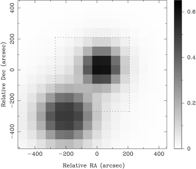
Figure 2: The true convergence distribution $\kappa(\mn@boldsymbol{\theta})=\Sigma(\mn@boldsymbol{\theta})/\Sigma_{\rm crit}$ of the model cluster. The dotted line indicates the edge of the observed field.

The cluster is simulated on a $16\times 16$ grid with a cell size of 1 arcmin and is everywhere subcritical. We then assume that the observed field consists only of the $8\times 8$ grid cells at the centre of the $16\times 16$ grid; this is delineated by the dashed box in Fig. 2.

In each cell of the observed field the average ellipticities and magnifications, in the absence of noise, are then calculated as follows. The complex ellipticity of an image is defined as

$$\epsilon=\epsilon_{1}+\mbox{i}\epsilon_{2}=\frac{a-b}{a+b}\exp(i\phi).$$

where $a$ and $b$ are respectively the lengths of the major and minor axes of the elliptical image and $\phi$ is its position angle with respect to the $x$-axis. If we assume that the intrinsic ellipticities of the background sources within a cell average to zero, then using (6) the predicted average ellipticities $\epsilon^{\rm(p)}_{i}$ $(i=1,2)$ in the cell due to lensing by the cluster are given simply by the mean values of $\gamma_{i}/(1-\kappa)$ over the cell, where $\gamma_{i}$ is calculated using (16). The predicted average magnification $\mu^{\rm(p)}$ in each grid cell can be calculated in a similar way, but in practice it is more convenient to work in terms of its inverse $r^{\rm(p)}$, which from (7) is given simply by the average of $(1-\kappa)^{2}-|\gamma|^{2}$ over the cell.

Finally, random Gaussian noise is added to the predicted average ellipticities and inverse magnifications in each cell. For the ellipticities, the standard deviation of the noise on each grid cell is assumed to be $\sigma_{\epsilon}=0.05$ and for the inverse magnifications we assume $\sigma_{r}=0.1$. The value $\sigma_{\epsilon}=0.05$ is consistent with that expected for 20 galaxies per grid cell (Schneider & Seitz 1995). If found from galaxy counts, the estimate of the magnification will be subject to Poisson noise, and for 30 galaxies per cell the error will be of the order of 10 per cent, and the noise on the inverse magnification will also be of the same size. Thus our assumption of an error $\sigma_{r}=0.1$ on the inverse magnification is not unreasonable.

Figure 3: Slices along the $x$ and $y$-axes for each of the observed quantities, $\epsilon_{1}$, $\epsilon_{2}$ and $r$. The continuous line is the quantity calculated directly from the mass distribution, with no noise added. The points are observed values of each quantity for a particular noise realisation. The error bars indicate the noise levels used.

Thus the basic data in our simulated lensing observation consist of, in each grid cell, the ‘observed’ average ellipticities $\epsilon^{\rm(o)}_{1}$ and $\epsilon^{\rm(o)}_{2}$ and inverse magnification $r^{\rm(o)}$, each of which contains a noise contribution. As an illustration of the simulated lensing data, in Fig. 3 we plot the average ellipicity and inverse magnification produced by our model cluster along the $x$ and $y$-axes in Fig. 2. The solid line represents the value of each quantity in the absence of noise, the points denote the observed values for our given noise realisation and the error bars indicate the rms noise level assumed.

4 The maximum-entropy method

As explained in the previous section, the simulated ‘observed’ data consist of the three quantities $\epsilon^{\rm(o)}_{1}$, $\epsilon^{\rm(o)}_{2}$ and $r^{\rm(o)}$ in each grid cell of the observed field. Let us denote these observed data by the vector

$${\textbf{{d}}}_{\rm o}=(\epsilon^{\rm(o)}_{1}(1),\epsilon_{2}^{\rm(o)}(1),r^{\rm(o)}(1),\ldots,\epsilon_{1}^{\rm(o)}(N),\epsilon_{2}^{\rm(o)}(N),r^{\rm(o)}(N)),$$

where $\epsilon_{1}^{\rm(o)}(j)$ and $\epsilon_{2}^{\rm(o)}(j)$ denote the observed components of the average ellipticity in the $j$th grid cell and $r^{\rm(o)}(j)$ denotes the corresponding observed inverse magnification. The total number of observed grid cells is $N=8\times 8=64$ in our simulation and thus the vector ${\textbf{{d}}}_{\rm o}$ has $3N=192$ components.

From these data, we wish to reconstruct the cluster mass distribution (defined in terms of the convergence $\kappa$) on some grid of points. For simplicity we use the same grid for the reconstruction as that on which the cluster mass distribution was originally defined (see Fig. 2), although this is not required by the algorithm. Hence we aim to reconstruct the convergence digitised on to $16\times 16$ cells and we denote this distribution by the vector

$$\mn@boldsymbol{\kappa}=(\kappa(1),\kappa(2),\ldots,\kappa(L)),$$

where $\kappa(j)$ is the convergence in the $j$th cell and $L$ is the total number of pixels in the reconstruction grid (i.e. $16\times 16$). Since the observed field consists only of the central $8\times 8$ grid cells, we are therefore attempting to reconstruct the cluster mass distribution some way outside the region in which data are available.

We choose our estimator $\hat{\mn@boldsymbol{\kappa}}$ of the convergence distribution to be that which maximises the posterior probability $\Pr(\mn@boldsymbol{\kappa}|{\textbf{{d}}}_{\rm o})$. Using Bayes’ theorem, this is given by

$$\Pr(\mn@boldsymbol{\kappa}|{\textbf{{d}}}_{\rm o})=\frac{\Pr({\textbf{{d}}}_{\rm o}|\mn@boldsymbol{\kappa})\Pr(\mn@boldsymbol{\kappa})}{\Pr({\textbf{{d}}}_{\rm o})},$$ (18)

where $\Pr({\textbf{{d}}}_{\rm o}|\mn@boldsymbol{\kappa})$ is the likelihood of obtaining the data given a particular convergence distribution and the evidence $\Pr({\textbf{{d}}}_{\rm o})$ is simply a constant that ensures the posterior probability is correctly normalised. The prior probability $\Pr(\mn@boldsymbol{\kappa})$ codifies our expectations about the convergence distribution before acquiring the data ${\textbf{{d}}}_{\rm o}$. Since the evidence is merely normalisation factor, we actually need only to maximise the product $\Pr({\textbf{{d}}}_{\rm o}|\mn@boldsymbol{\kappa})\Pr(\mn@boldsymbol{\kappa})$.

Let us first consider the form of the likelihood $\Pr({\textbf{{d}}}_{\rm o}|\mn@boldsymbol{\kappa})$. As discussed above, given a convergence distribution $\mn@boldsymbol{\kappa}$ we can use equations (16) and (7) to predict the values of the noiseless average ellipticities and inverse magnification in each observed grid cell. We denote these predicted values in the $j$th grid cell as $\epsilon_{1}^{\rm(p)}(j)$, $\epsilon_{2}^{\rm(p)}(j)$ and $r^{\rm(p)}(j)$ and assemble the values for all the cells into the predicted data vector

$${\textbf{{d}}}_{\rm p}=(\epsilon^{\rm(p)}_{1}(1),\epsilon_{2}^{\rm(p)}(1),r^{\rm(p)}(1),\ldots,\epsilon_{1}^{\rm(p)}(N),\epsilon_{2}^{\rm(p)}(N),r^{\rm(p)}(N)).$$

Therefore, we may consider the observed data vector as

$${\textbf{{d}}}_{\rm o}={\textbf{{d}}}_{\rm p}+{\textbf{{n}}},$$

where the vector n contains the noise contribution in each observed grid cell for our particular realisation.

If the noise on the observed data values is Gaussian-distributed then the likelihood function is the $3N$-dimensional multivariate Gaussian

$$\Pr({\textbf{{d}}}_{\rm o}|\mn@boldsymbol{\kappa})\propto\exp\left[-{\textstyle\frac{1}{2}}({\textbf{{d}}}_{\rm o}-{\textbf{{d}}}_{\rm p})^{\rm T}{\textbf{{N}}}^{-1}({\textbf{{d}}}_{\rm o}-{\textbf{{d}}}_{\rm p})\right],$$

where ${\textbf{{N}}}=\langle{\textbf{{n}}n}^{\rm T}\rangle$ is the ensemble average noise covariance matrix. If there are any correlations between the different measured quantities, either within a cell or between cells, then they can be straightforwardly incorporated into the noise covariance matrix. For example, Bartelmann et al. (1996) point out that for faint lensed images it is possible that the measured values of the ellipticities and magnification can be correlated. In most cases, however, it is assumed that the data values are all independent, so the noise covariance matrix becomes diagonal and is given by

$${\textbf{{N}}}=\mbox{diag}(\sigma^{2}_{d(1)},\ldots,\sigma^{2}_{d(3N)}),$$

where $\sigma^{2}_{d(j)}$ is the variance of the noise in the $j$th data value. Then the likelihood becomes

$$\Pr({\textbf{{d}}}_{\rm o}|\mn@boldsymbol{\kappa})\propto\exp\left(-{\textstyle\frac{1}{2}}\chi^{2}\right),$$ (19)

where $\chi^{2}$ is the standard misfit statistic given by

$$\chi^{2}=\sum_{j=1}^{3N}\frac{\left[d_{\rm o}(j)-d_{\rm p}(j)\right]^{2}}{\sigma^{2}_{d(j)}}.$$ (20)

Let us now turn our attention to the prior probability $\Pr(\mn@boldsymbol{\kappa})$. The simplest possible prior is the uniform prior, which assumes that in each grid cell, before acquiring any data, all values of the convergence are equally likely. In this case the posterior probability is directly proportional to the likelihood and so by maximising the posterior with respect to $\mn@boldsymbol{\kappa}$, we actually obtain the maximum-likelihood estimator for the convergence distribution. However, since the convergence is a positive additive distribution, it may be shown (Skilling 1989), using very general notions of subset invariance, coordinate invariance and system independence, that the prior probability assigned to the components of the vector $\mn@boldsymbol{\kappa}$ should take the form

$$\Pr(\mn@boldsymbol{\kappa})\propto\exp[\alpha S(\mn@boldsymbol{\kappa},{\textbf{{m}}})],$$ (21)

where the dimensional constant $\alpha$ depends on the scaling of the problem and may be considered as a regularising parameter, and m is a model vector to which $\mn@boldsymbol{\kappa}$ defaults in the absence of any evidence in the data to the contrary. The function $S(\mn@boldsymbol{\kappa},{\textbf{{m}}})$ is the cross-entropy of $\mn@boldsymbol{\kappa}$ and m and is given by

$$S(\mn@boldsymbol{\kappa},{\textbf{{m}}})=\sum_{j=1}^{L}\kappa(j)-m(j)-\kappa(j)\ln\left(\frac{\kappa(j)}{m(j)}\right),$$ (22)

which has a global maximum at $\mn@boldsymbol{\kappa}={\textbf{{m}}}$. If we have some prior knowledge of the structure of the lensing cluster, we may include this information in the model m. Otherwise, we set the model to have the same value in each pixel. This value is generally set to be somewhat smaller than the level expected for the reconstructed convergence distribution, but in regions where the convergence is well-constrained by the data, the level of the model makes no difference to the final reconstruction (see Section 6).

Combining the expression (19) and (21) for the likelihood and prior respectively, we see that the posterior probability distribution is given by

$$\Pr(\mn@boldsymbol{\kappa}|{\textbf{{d}}}_{\rm o})\propto\exp(-{\textstyle\frac{1}{2}}\chi^{2}+\alpha S).$$ (23)

Therefore, maximising this distribution with respect to $\mn@boldsymbol{\kappa}$ is equivalent to minimising the function

$$F={\textstyle\frac{1}{2}}\chi^{2}-\alpha S.$$ (24)

From the expressions (20) and (22), it is possible to calculate analytically the first and second partial derivatives of $F$ with respect to $\kappa(j)$ ($j=1,2,\ldots,L$). In order to minimise the function $F$ we use a conjugate gradient algorithm in which the analytical derivative calculations are performed using Fast Fourier Transforms. Specifically, we use the Polak-Ribiere variant of Fletcher-Reeves conjugate gradient method (Press et al. 1992), with modifications to the implementation as suggested by Mackay (1996). In fact, since the convergence distribution is always positive it is convenient to minimise with respect to $\log\kappa(j)$ for which the corresponding derivatives of $F$ are also easily found.

Finally, we must consider the value of the regularising parameter $\alpha$. In early implementations of MEM, $\alpha$ was chosen so that for the final reconstruction the misfit statistic $\chi^{2}$ equalled its expectation value, i.e. the number of data values $3N$. This choice is usually refered to as historic MEM. It is, however, possible to determine the appropriate value for $\alpha$ in a fully Bayesian manner (Skilling 1989; Gull & Skilling 1990) by simply treating it as another parameter in our hypothesis space. It may be shown that $\alpha$ must satisfy

$$-2\alpha S(\hat{\mn@boldsymbol{\kappa}},{\textbf{{m}}})=L-\alpha\mbox{Tr}({\textbf{{M}}}^{-1}),$$ (25)

where $\hat{\mn@boldsymbol{\kappa}}$ is the convergence distribution that minimises the function $F$ for this value of $\alpha$ and $L$ is the total number of pixels in the reconstruction. The $L\times L$ matrix M is given by

$${\textbf{{M}}}={\textbf{{G}}}^{-1/2}{\textbf{{H}}}{\textbf{{G}}}^{-1/2},$$

where ${\textbf{{H}}}=\nabla_{\mn@boldsymbol{\kappa}}\nabla_{\mn@boldsymbol{\kappa}}F$ is the Hessian matrix of the function $F$ evaluated at the point $\hat{\mn@boldsymbol{\kappa}}$ and ${\textbf{{G}}}=-\nabla_{\mn@boldsymbol{\kappa}}\nabla_{\mn@boldsymbol{\kappa}}S$ is minus the Hessian matrix of the entropy function at $\hat{\mn@boldsymbol{\kappa}}$. As mentioned above, these matrices can be calculated analytically.

It may also be shown, however, that the Bayesian value for $\alpha$ may be reasonably well approximated by simply choosing its value such that the value of $F$ at its minimum is equal to the half number of data points, i.e. $F(\hat{\mn@boldsymbol{\kappa}})=3N/2$ (see Mackay 1996). We have determined $\alpha$ by both methods and found them to agree to within a few percent. More importantly, the resulting reconstructions of the convergence distributions for each case are indistinguishable.

5 Estimating the reconstruction errors

It is essential to be able to estimate the errors in the reconstruction. From (23) and (24), we see that the posterior probability distribution may be written

$$\Pr(\mn@boldsymbol{\kappa}|{\textbf{{d}}}_{\rm o})\propto\exp[-F(\mn@boldsymbol{\kappa})].$$

In general, the posterior distribution may have a complicated shape. Nevertheless, we may approximate its shape near the peak $\hat{\mn@boldsymbol{\kappa}}$ by a Gaussian of the form

$$\Pr(\mn@boldsymbol{\kappa}|{\textbf{{d}}}_{\rm o})\propto\exp\left[-{\textstyle\frac{1}{2}}(\mn@boldsymbol{\kappa}-\hat{\mn@boldsymbol{\kappa}})^{\rm T}{\textbf{{H}}}(\mn@boldsymbol{\kappa}-\hat{\mn@boldsymbol{\kappa}})\right],$$ (26)

where H is the Hessian matrix mentioned above. Comparing (26) with the standard form for a multivariate Gaussian distribution, we see that the covariance matrix of the errors on the $\mn@boldsymbol{\kappa}$ reconstruction are given approximately by the inverse of the Hessian matrix, i.e.

$$\langle(\mn@boldsymbol{\kappa}-\hat{\mn@boldsymbol{\kappa}})(\mn@boldsymbol{\kappa}-\hat{\mn@boldsymbol{\kappa}})^{\rm T}\rangle\approx{\textbf{{H}}}^{-1},$$ (27)

where the angle brackets denote the ensemble average. The Hessian matrix at the peak of the posterior distribution can be calculated analytically and has dimension $L\times L$, where $L$ is the total number of pixels in the reconstruction. In our simulation $L=256$, and so the numerical inversion of the matrix may be performed using standard techniques in just a few seconds of CPU time. This therefore provides a quick approximation to the covariance matrix of the reconstruction errors.

In order for the above method to be reliable, we require the Gaussian approximation at the peak of the posterior distribution to be reasonably accurate. An alternative method for estimating the errors on the reconstruction, which does not rely on any approximations, is to use Monte-Carlo simulations. By repeating the analysis of the same lensing data many times, but using different noise realisations, we can measure the covariances of the reconstruction errors numerically. However, this technique only provides an estimate of the ensemble average errors, rather than the errors associated with the reconstruction obtained from particular noise realisation. In addition, this approach is more computationally intensive.

6 Application to simulated observations

We have applied the MEM approach to the simulated ellipticity and magnification data discussed in Section 3, which were produced assuming the cluster convergence distribution shown in Fig. 2. Assuming the model m in (22) to have a uniform value of 0.02 across the whole field, the resulting MEM reconstruction of the convergence distribution is shown in Fig. 4. This reconstruction converges after about 90 iterations of the conjugate gradient algorithm to the point where the fractional change in $F$ per iteration is less that 0.1 per cent. The total CPU time required is about 2 minutes on a Sparc Ultra workstation. The Bayesian value of the regularising parameter $\alpha$ that satisfies (25) was found to be $\alpha=2.6$, On performing a further 100 iterations to achieve an even more tightly defined convergence, the fractional change in $F$ per iteration decreases to only 0.001 per cent and, more importantly, this makes no discernable difference to the reconstruction. Similar performances were found for numerous other noise realisations and we are therefore confident that the MEM solution is extremely stable.

Comparing the reconstruction with the true distribution shown in Fig. 2, we see that within the observed field (delineated by the dashed box), the MEM reconstruction has faithfully reproduced the main features. In the first layer of pixels outside the box some spurious features occur but, as discussed below, these are easily shown not to be significant. The algorithm succeeded in reconstructing the mass condensation to the bottom left of the observed field. This feature in the reconstruction is in fact found to be significant, despite the fact that much of it lies outside the observing box. We also note that the entropic regularisation of the reconstruction has resulted in the outer edges defaulting to the model value in the absence of any data to the contrary.

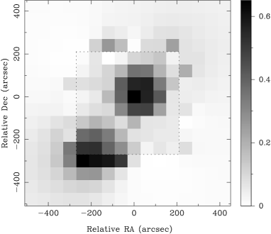
Figure 4: The maximum-entropy reconstruction of the convergence distribution of the model cluster shown in Fig. 2. The dotted line indicates the edge of the observed field.

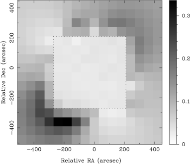
Figure 5: The rms errors in the MEM reconstruction of the cluster convergence, as estimated by making a Gaussian approximation to the posterior probability distribution at its peak. The dotted line indicates the edge of the observed field.

One may investigate the accuracy of the reconstruction and the significance of various features using either of the techniques discussed in Section 5. First, we use the Gaussian approximation to the posterior probability distribution to estimate the covariance matrix of the reconstruction errors. The square-root of the diagonal elements of this matrix give the rms errors in the reconstruction in each grid cell, and these are plotted in Fig. 5. Comparing this with the MEM reconstruction shown in Fig. 4 and the true convergence distribution in Fig. 2, we see that the rms errors are uniformly low within the observing box, with a typical value of about 0.05. Outside the observing box the rms errors increase, as expected. In particular, we see that rms errors are indeed highest in the grid cells where the reconstruction differs most noticeable from the true distribution.

As a further illustration of the accuracy of the reconstruction, in Fig. 6 we plot slices along the $x$ and $y$-axes for the true convergence distribution (solid line) and the MEM reconstruction (points); we also plot the rms errors on the reconstruction predicted by the Gaussian approximation to the posterior distribution. In addition to reconstruction discussed above, for which the level of the flat model m was set to 0.02, Fig. 6 also contains similar plots for reconstructions calculated from the same lensing data, but for which the models levels were set to 0.002 and 0.2 respectively. These plots show that within the observing box the level of the model makes virtually no difference to the reconstruction. Outside the observing box, we see that, as expected, the reconstruction tends to the model value in regions where there is no evidence in the data to the contrary. More importantly, we see that in all the plots shown in Fig. 6 the difference between the true and reconstructed distributions is consistent with the calculated error bars.

As mentioned in Section 5, we may also investigate the accuracy of the MEM reconstruction by performing Monte-Carlo simluations in which the same lensing data are analysed but for different noise realisations. In Fig. 7 we plot the results obtained for 100 Monte-Carlo realisations, in the same format as Fig. 6. The points denote the mean reconstructed convergence obtained in each grid cell averaged over the 100 realisations. The errors bars denote the standard deviation of the convergence in each grid, as measured directly from the realisations. In regions where the convergence distribution is well-determined by the observations, we see that the mean reconstructed value is very close to the true distribution, indicating that there no bias in the MEM reconstruction. Moreover, in the observed field, the sizes of the error bars agree closely with those in Fig. 6, which shows that the Gaussian approximation to the posterior probability distribution is quite accurate. In regions where the data do not constrain the convergence, we see that the reconstruction always defaults to the assumed model level and hence the ensemble-average error bars are very small.

Figure 6: Slices through the $x$ and $y$ axes of the convergence distribution. The continuous line is the true distribution and the points are the reconstructed values. The error bars show the standard deviation of the reconstruction errors in each cell, as estimated by making a Gaussian approximation to the peak of the posterior probability distribution.

Figure 7: Slices through the $x$ and $y$ axes of the convergence distribution. The continuous line is the true distribution and the points are the mean values of the convergence in each cell averaged over 100 noise realisations. The error bars show the standard deviations of the convergence in each cell calculated directly from the 100 reconstructions using different noise realisations.

In addition we have carried out a ‘noise power analysis’ like that of Seitz & Schneider (1996) and Squires & Kaiser (1996). In Fig. 8 (a) we plot the azimuthal average of the 2D power spectrum of the residuals between the reconstructed field and the original field (taken within the observed field only), averaged over 100 noise realisations. The $k=0$ power point is due to the square of the mean of the residual map, averaged over realisations. However, apart from this point, the power is low for small $k$ and increases for large $k$. This reflects the fact that the uncertainties in the mass densities of neighbouring pixels are strongly correlated, but the errors in widely spaced pixels are not. This is more easily seen in the auto correlation function of the residual map plotted in Fig. 8 (b). As expected, the errors in directly neighbouring pixels are slightly anti-correlated since the effect on the shear of adding mass density to one pixel is partially cancelled out by taking away mass density from a neighbouring pixel. However the autocorrelation function tends to zero as the pixel separations increases, indicating that there are negligible long-wavelength correlations in the errors.

Figure 8: The azimuthally averaged power spectrum (a) and autocorrelation function (b) of the residuals (reconstructed convergence minus true convergence) in the observed field averaged over 100 noise realisations. The error bars show the 1–sigma uncertainties in each point as derived from the 100 realisations. The plotted power spectrum is the azimuthal average of the 2D power spectrum of the residuals map. The normalisation was taken such that the sum of the points in the 2D power spectrum equalled the mean squared value of the residuals map. The normalisation of the autocorrelation function was fixed so that it equalled unity at zero separation.

Finally, for comparison with the MEM reconstruction shown in Fig. 4, we calculate the maximum-likelihood (i.e. $\alpha=0$) reconstruction obtained using the same lensing data. The resulting reconstruction is shown in Fig. 9, after 160 iterations of the conjugate gradient minimisation algorithm at which point the fractional change in $F$ per iteration is 0.1 per cent. The reconstruction is plotted on the same greyscale as Figs 2 and 4, in order to illustrate that in the observed field the result is similar to the maximum-entropy reconstruction. Outside the observed field, however, there are numerous spurious features in which the convergence rises to unrealistically large values, with a peak value of about 1.3. Also the condensation of mass to the bottom left of the field is not faithfully reconstructed outside the observed box. Moreover, on iterating further, the peak value of the reconstructed convergence distribution continues to rise, and after 800 iterations the fractional change in $F$ per iteration is less than 0.001 per cent and the peak convergence is 2.3. After an additional 800 iterations the peak convergence rises to 4.0, although the fractional change per iteration in the value of $F$ becomes extremely small. For other noise realisations, we sometimes found the maximum-likelihood solution to be even less stable and, in some cases, the peak value of the reconstructed convergence distribution continued to rise steadily beyond 1500 iterations to values exceeding 7.0. Thus, outside the observing box we find that the maximum-likelihood reconstruction does not, in general, converge to a numerically stable solution. As discussed in Section 4, we further note that the maximisation of the likelihood function is performed with respect to $\log\kappa(j)$. Thus, the algorithm used to calculate the maximum-likelihood reconstruction already enforces positivity and may therefore be compared directly with more sophisticated reconstruction methods such as the Lucy-Richardson algorithm. We would therefore expect such methods also to suffer from similar numerical instabilities.

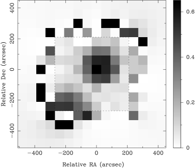
Figure 9: The maximum likelihood reconstruction of the model cluster convergence distribution. The dotted line indicates the edge of the observed field.

7 Conclusions

We have presented a new maximum-entropy method for reconstructing the projected mass distribution galaxy cluster from observations of its gravitational lensing effects. The method is ideally suited to the reconstruction of clusters for which the observing field is small or irregularly-shaped and does not suffer from unwanted boundary effects that affect the reconstructions obtained using the traditional Kaiser & Squires algorithm. We find that for realistic levels of uncertainty in the observed shear and magnification patterns, the technique faithfully reproduces the cluster mass distribution within the observed field and, moreover, yields a reasonable reconstruction some distance beyond the observing box. We also show that the errors on the reconstruction can be reliably estimated by making a Gaussian approximation to the posterior probability distribution at its peak. In regions where the cluster mass distribution is well constrained by the lensing observation, we find that the estimated reconstruction errors agree well with those obtained from Monte-Carlo simulations.

ACKNOWLEDGMENTS

We thank David Mackay for several helpful suggestions. SLB acknowledges the PPARC for support in the form of Research Studentship.

References

- [1] Bartelmann M., 1995, A&A, 303, 643
- [2] Bartelmann M., Narayan R., 1995, ApJ, 451, 60
- [3] Bartelmann M., Narayan R., Seitz S., Schneider P., 1996, ApJ, 464, L115
- [4] Blandford R.D., Narayan R., 1992, ARAA, 30, 311
- [5] Broadhurst T., Taylor A., Peacock J., 1995, ApJ, 438, 49
- [6] Falco E.E., Gorenstein M.V., Shapiro I.I., 1985, ApJ, 289, L1
- [7] Fort B., Mellier Y., 1994, A&AR, 5, 239
- [8] Gull S. F., 1989, in Skilling J., ed., Maximum Entropy and Bayesian Methods. Kluwer, Dordrecht, p. 53
- [9] Gull S.F., Skilling J., 1990, The MEMSYS5 Users’ Manual. Maximum Entropy Data Consultants Ltd, Royston.
- [10] Kaiser N., 1995, ApJ, 439, L1
- [11] Kaiser N., Squires G., 1993, ApJ, 404, 441
- [12] Kaiser N., Squires G., Broadhurst T., 1995, ApJ, 449, 460
- [13] Kneib J.-P., Mathez G., Fort B., Mellier Y., Soucail G., Longaretti P.-Y., 1994, A&A, 286, 701
- [14] Kochanek C.S., 1990, MNRAS, 247, 135
-
[15]
Mackay D.J.C.,
http://wol.ra.phy.cam.ac.uk/mackay/c/macopt.html. - [16] Miralda-Escudé J., ApJ, 370, 1
- [17] Narayan R., Bartelmann M., 1996, astro-ph/9606001
- [18] Press W.H., Teukolsky S.A., Vettering W.T., Flannery B.P., 1992 in Numerical Recipes, 2nd. Ed. Cambridge: Cambridge Univ. Press.
- [19] Schneider P., Ehlers J., Falco E.E., 1992, in Gravitational lenses. Astronomy and Astrophysics Library, New York, Berlin: Springer
- [20] Schneider P., Seitz C., 1995, A&A, 294, 411
- [21] Seitz C., Schneider P., 1997, A&A, 318, 687
- [22] Seitz S., Schneider P., 1996, A&A, 305, 383
- [23] Seitz S., Schneider P., Bartelmann M., 1998, astro-ph/9803038
- [24] Skilling J., 1989, in Skilling J., ed., Maximum Entropy and Bayesian Methods. Kluwer, Dordrecht, p. 45
- [25] Smail I., Ellis R.S., Fitchett M.J., 1994, MNRAS, 273, 277
- [26] Squires G., Kaiser N., 1996, ApJ, 473, 65
- [27] Tyson J.A., Valdes F., Wenk R.A., 1990, ApJ, 349, L1
- [28] Woods D., Fahlman G.G., Richer H.B., 1995, ApJ, 454, 32