Exact Solution of the Kompaneets Equation for Strong Explosion in Medium with Inverse-Square Decreasing Density

Abstract

In the framework of the Kompaneets approximation the propagation of a shock front (SF) in inhomogeneous medium with the power-law density decrease at the exponent $n=2$ is investigated. For this important case corresponding to outer regions of the solar and stellar coronas an unexpectedly simple exact solution clearing a structure of the general solution for an arbitrary monotonic density of medium is found. Our results for plane-layered medium are compared to the Korycansky one for off-centre explosion in radially stratified medium. The relation between the solutions in these media are found and a new exact solution for a noncentral explosion in the case of density singularity on the finite radius is received.

Introduction

As really seen from the well-known Sedov–Tailor formula in the homogeneous medium [1, 2]

$$R=[E_{0}t^{2}/\rho_{0}]^{1/5}$$ (1)

for the dependence of the radius $R$ of a shock front on time $t$ from the moment of explosion, the explosion energy $E_{0}$ and the medium density $\rho_{0}$, the SF would move faster towards the direction of density decrease if explosion occurs in inhomogeneous medium. However, for inhomogeneous medium the problem becomes more complicated, being not self-similar, and requires significantly more complicated calculations even for computational analysis (see the review and papers [3, 4, 5] and the bibliography therein).

Assuming the uniform pressure along the envelope behind the SF A. S. Kompaneets proposed the equation [6] (see Eq. (3) below) for strong explosion in an exponential atmosphere. In that case he was showed that the SF was accelerated and could get infinity for a finite time. (Surely, the approximation fails earlier and account for a non zero density at infinity [7] restricts values of the SF velocity too, i.e., there is no controversy with physics or common sense.) For densities decreasing not so fast, namely, for the power-law density dependence $\rho(z)\propto z^{-n}$, often met in astrophysical objects, the behaviour of the SF is defined by the exponent $n$ [2, 8, 9]. The asymptotically exact solution for the head part of the SF moving towards the direction of density decrease indicates that the Sedov–Tailor SF deceleration is down when the density gradient (or $n$) is up. Particularly, it is confirmed by the exact solution of the Kompaneets equation discussed below for $n=2$ [12] corresponding to the wind regions in outer parts of the solar and stellar coronas (however, with the wind motion not taken into account). This solution having an extremely simple form is analysed in this publication.

Following Kompaneets [6], instead of the real time $t$ we define the new temporal variable $y$ as

$$dy=dt[E_{0}\lambda(\gamma^{2}-1)/(2\rho_{0}V(t))]^{1/2},$$ (2)

including into it the inverse square root of the time dependent volume $V(t)=\pi\int r^{2}\,dz$. After substitution the coefficients of the equation for the SF $r=r(y,z)$ do not depend on time any more but only on the coordinate $z$. Along this coordinate the density changes as $\rho(z)=\rho_{0}/(z/z_{0})^{2}$. Here $\rho_{0}$ is the unperturbed density in the point of explosion $z_{0}$. Some another relations important for applications but not for the current formal consideration are presented in Appendix 1. The Kompaneets equation for the shock front can be written as:

$$(\partial r/\partial y)^{2}\varphi(z)-[(\partial r/\partial z)^{2}+1]=0.$$ (3)

Here $\varphi(z)=\rho(z)/\rho_{0}$. In the case of $n=2$ the solution could be immediately written, however, we will consider it as a particular case of the general situation to clarify its structure in more general cases of astrophysical interest (change of the exponent $n$ from 16 to 6 and 2 in the solar corona; $n=3$ in active nuclei of galaxies).

The plan of this paper is the following. In the beginning we give the quadrature parametric solution of the Kompaneets equation (3) (see [6]) for an arbitrary density distribution of the medium using a supplementary function $\xi(y,z)$ and an arbitrary function $\mu(\xi)$. Regarding the medium at the initial stage of expansion as homogeneous we conclude from comparison to the Sedov solution that $\mu$ is to be zero (see [6]). At $\mu=0$ for the inverse-square law of the density decrease we find an explicit solution in two regions adjoined to the opposite leading points of the SF. In this two regions the solution consists of two non-adjoined segments of the same sphere. In the intermediate region the function $\mu$ is not zero as well as in the Silich & Fomin case [7], where the density decreases exponentially to some constant value. The solution obtained in the intermediate region complements the SF to a full sphere. It is shown that at short times ($y\to 0$) the intermediate region disappears. The transformation is also found of this solution in a plane-layered medium to that for an off-centre explosion in the radially stratified medium with the density distribution having a singularity at a sphere surface with a finite radius, i.e., one more new solution is obtained. (Preliminary comparison is carried out to the Korycansky solution [8] for a power-law radially-stratified medium). An extremely simple form of the solution obtained admits explicit calculations which can be important for general analysis of propagation of strongly non-linear waves in an inhomogeneous media. A square-root singularity at the leading points is revealed as an inherent feature of $\xi$ for an arbitrary density dependence on coordinates. This feature allows some conclusions to be made about SF properties. The fact is that different representations of the solution is required in different regions. Probably, in the vicinity of every leading point we deal with the only non-linear wave whereas contribution of both of these waves (non-linear “interference”) should be matched by choosing the function $\mu$ in the intermediate region.

Initial condition

The complete integral of Eq. (3) dependent on two arbitrary constants (according to the number of independent variables) can be found via separation of variables (see, for example, [13]). Regarding the integration constant $\mu$ as an arbitrary function of the separation constant $\xi$ and substituting the latter with the function of two independent variables $\xi(y,z)$, which can be derived from the condition [13]

$$dr/d\xi=0,$$ (4)

we find the following expression for the general integral:

$$r=-\mathop{\rm sign}\nolimits(z-z_{0})\int_{z_{0}}^{z}dx\sqrt{\xi^{2}\varphi(x)-1}+\xi y+\mu(\xi).$$ (5)

This general integral and the condition (3) for the function $\xi$ give its implicit expression via $z$ and $y$

$$y=\mathop{\rm sign}\nolimits(z-z_{0})\int_{z_{0}}^{z}dx\frac{\xi\varphi(x)}{\sqrt{\xi^{2}\varphi(x)-1}}-\mu^{\prime},\quad\frac{d\mu}{d\xi}\equiv\mu^{\prime},$$ (6)

from where for the solution describing the SF we have

$$r=\mathop{\rm sign}\nolimits(z-z_{0})\int_{z_{0}}^{z}\frac{dx}{\sqrt{\xi^{2}\varphi(x)-1}}+\mu-\xi\mu^{\prime}.$$ (7)

At $y\to 0$, $z\to z_{0},$ $r\to 0$,

$$r\approx\frac{1}{\sqrt{\xi^{2}-1}}\,|z-z_{0}|+\mu-\xi\mu^{\prime},\quad y\approx\frac{\xi}{\sqrt{\xi^{2}-1}}\,|z-z_{0}|-\mu^{\prime},$$ (8)

or

$$\left(\frac{r-\mu+\xi\mu^{\prime}}{{z-z_{0}}}\right)^{2}\approx\frac{1}{\xi^{2}-1},\quad\left(\frac{y+\mu^{\prime}}{z-z_{0}}\right)^{2}\approx\frac{\xi^{2}}{\xi^{2}-1}.$$ (9)

Generally, the supplementary functions $\mu$ and $\xi$ are considered not expanded. Excluding $\xi^{2}$ gives:

$$\left(\frac{r-\mu+\xi\mu^{\prime}}{z-z_{0}}\right)^{2}+1=\left(\frac{y+\mu^{\prime}}{z-z_{0}}\right)^{2}.$$ (10)

It is obvious that approaching the Sedov limit

$$r^{2}+(z-z_{0})^{2}=y^{2}$$ (11)

is possible only if (disregarding possible though non-essential shift of initial moment of explosion)

$$\frac{\xi\mu^{\prime}-\mu}{r}\to 0,\quad r\to 0;\quad\frac{\mu^{\prime}}{y}\to 0,\quad y\to 0.$$ (12)

Finally, for this limiting case of medium homogeneous at small distances the following relations occur

$$\mu^{\prime}=0,\quad\mu=0.$$

We will see below that the situation is more complicated, however, for while we can use the relations derived for the exponent of interest $n=2$.

Solution for $n=2$ in the vicinity of leading points

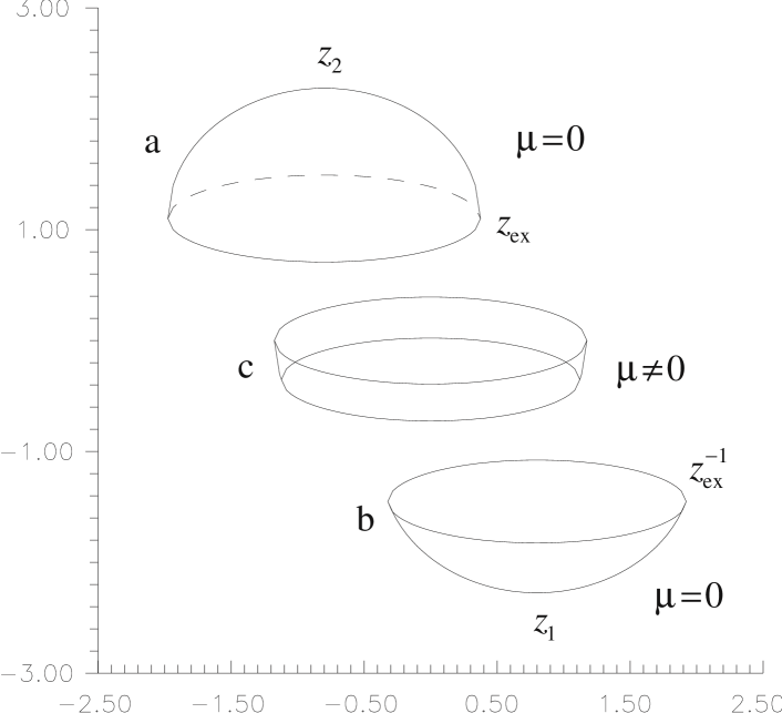
Figure 1: The sphere SF corresponding to strong explosion in a plane-layered medium with the inverse square density decrease. a) The half-sphere adjoined to the upper leading point $z_{2}(t)$ moving towards the density decrease. b) The surface of the sphere segment adjoined to the lower leading point $z_{1}(t)$. c) The surface of the spherical layer complementing the SF to the sphere. This part of the solution contrary to a) and b) corresponds to $\mu\neq 0$ (the region of the “interference” of waves). The parts of the SF corresponding to the solutions in different regions (see text) are shifted here each off another.

As mentioned above, this case is important for the astrophysical applications (outer parts of coronas, the Solar wind region, etc.). However, it also gives us a clear example of how to express the solution via supplementary functions. At $\varphi(z)=1/z^{2}$ $(z_{0}=1)$ the integrals are expressed via elementary functions but, as seen, separate regions in the $z,y$ plane should be considered to provide positiveness of the expressions under the square root. Let $z$ satisfy the inequality $z_{2}>z>z_{\rm ex}$. In this region adjacent to the leading point of the SF we obtain ($\mu=0$):

$$\xi^{2}\varphi>1,\quad\xi\mid_{z_{\rm ex}}=z_{\rm ex},\quad(z_{0}=1),$$

$$r=\sqrt{\xi^{2}-1}-\sqrt{\xi^{2}-z^{2}},\quad(z>1),$$ (13)

$$\xi^{2}=\frac{z^{2}(1-e^{2y})^{2}}{4e^{2y}(e^{y}-z)(z-e^{-y})}.$$ (14)

Here

$$z_{2}=e^{y},\quad z_{1}=e^{-y},\quad z_{\rm ex}=\cosh y,\quad r\mid_{z_{\rm ex}}=\sinh y.$$ (15)

Calculating

$$\xi^{2}-1=\frac{[z(1+e^{2y})-2e^{y}]^{2}}{4e^{2y}(e^{y}-z)(z-e^{-y})}\quad,$$ (16)

and

$$\xi^{2}-z^{2}=\frac{z^{2}(1+e^{2y}-2ze^{y})^{2}}{4e^{2y}(e^{y}-z)(z-e^{-y})}$$ (17)

we find that

$$z>z_{\rm ex},\quad\sqrt{\xi^{2}-z^{2}}=\frac{z(z-z_{\rm ex})}{\sqrt{(z_{2}-z)(z-z_{1})}}>0,\quad\xi\mid_{z_{\rm ex}}=z_{\rm ex}.$$ (18)

$$z>z_{\rm ex}^{-1},\quad\sqrt{\xi^{2}-1}=\frac{zz_{\rm ex}-1}{\sqrt{(z_{2}-z)(z-z_{1})}},\quad\xi\mid_{z_{\rm ex}^{-1}}=1.$$ (19)

Substituting these relations into Eq. (13) we get an extremely simple solution:

$$r=\sqrt{(z_{2}-z)(z-z_{1})}\quad,\quad z_{2}>z>z_{\rm ex}.$$ (20)

Apparently, it is the equation of the hemisphere hanging on the upper leading point $z_{2}$ with the centre at $z_{\rm ex}$ and radius $(z_{2}-z_{1})/2$ (Fig. 1a). Note that in this region really $\xi>z$ (17). At $z_{1}<z<z_{\rm ex}^{-1}<1$ with $\xi^{2}$ from (14) we have

$$r=\sqrt{\xi^{2}-z^{2}}-\sqrt{\xi^{2}-1},$$ (21)

$$\sqrt{\xi^{2}-z^{2}}=\frac{z(z_{\rm ex}-z)}{\sqrt{(z_{2}-z)(z-z_{1})}}\quad,\quad\sqrt{\xi^{2}-1}=\frac{1-zz_{\rm ex}}{\sqrt{(z_{2}-z)(z-z_{1})}},$$ (22)

and, finally, (Fig. 1b) the solution reduced to the same form

$$r=\sqrt{(z_{2}-z)(z-z_{1})},\quad zz_{\rm ex}<1$$

describes the segment surface of the same sphere leaning against the lower leading point $z_{1}$. The square root singularities of $\xi$ at the leading points are the general property for an arbitrary $n$ substantially used in [9].

Intermediate region

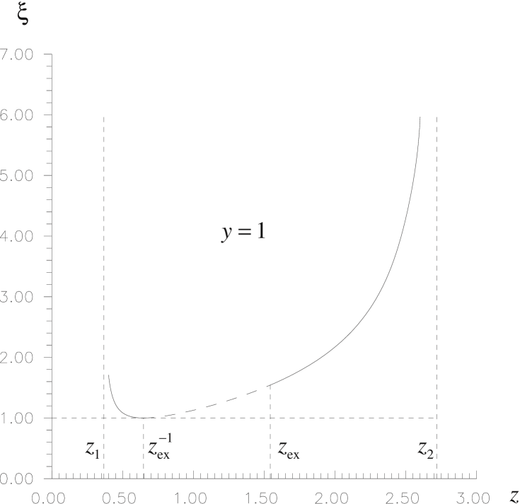
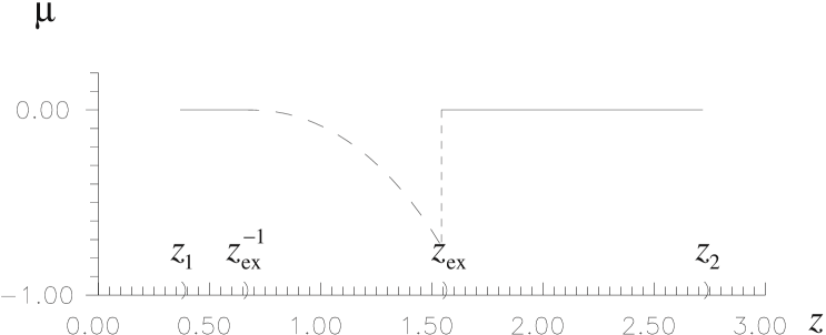
Figure 2: The supplementary functions $\xi$ and $\mu$ parameterising the solution for the SF. The square-root singularities of $\xi$ at the leading points arise for an arbitrary $n$.

Here we return to the initial general form of the solution with the arbitrary function which is found from matching conditions at the boundary between the regions (compare to Silich & Fomin [7])

$$r\mid_{z_{\rm ex}-0}=r\mid_{z_{\rm ex}+0},\quad(z_{\rm ex}=\xi\mid_{z_{\rm ex}})$$ (23)

$$\mu(\xi)=2\sqrt{\xi^{2}-1}-2\xi\ln\left\{\xi+\sqrt{\xi^{2}-1}\right\}$$ (24)

$$\mu^{\prime}(\xi)=-2\ln\left\{\xi+\sqrt{\xi^{2}-1}\right\}$$ (25)

Substituting these relations into

$$0=\frac{\partial r}{\partial\xi}=\int_{1}^{z}\frac{\xi\varphi\,dx}{\sqrt{\xi^{2}\varphi-1}}+y+\mu^{\prime}(\xi)$$ (26)

we get the equation for $\xi$ at $z_{\rm ex}>z>z_{\rm ex}^{-1}$

$$y=\ln\left|\frac{\xi+\sqrt{\xi^{2}-z^{2}}}{z}(\xi+\sqrt{\xi^{2}-1})\right|.$$ (27)

Using the definition

$$\xi\equiv\cosh\alpha$$ (28)

we obtain

$$\alpha=\ln\sqrt{\frac{z_{2}(zz_{2}-1)}{(z_{2}-z)}},$$ (29)

$$\alpha\mid_{z_{\rm ex}}=y,\quad\alpha\mid_{z_{\rm ex}^{-1}}=0.$$

Thus, the value $\xi$ (Fig. 2a) in this region is given by the relation

$$\xi\mid_{z_{\rm ex}}=\cosh y=z_{\rm ex},\quad\xi\mid_{z_{\rm ex}^{-1}}=1.$$ (30)

$$\xi=\cosh\ln\sqrt{\frac{e^{y}(e^{y}z-1)}{e^{y}-z}},\quad z_{\rm ex}>z>z_{\rm ex}^{-1}.$$ (31)

It is seen that

$$\mu_{z_{\rm ex}^{-1}}=\mu_{z_{\rm ex}^{-1}}^{\prime}=0,$$ (32)

$$\mu\neq 0,\quad\mu^{\prime}\neq 0\quad(z=z_{\rm ex}).$$

Therefore $\mu$ is continuous at the lower boundary but together with the first derivative it jumps at the upper one (Fig. 2b).

$$\mu(\xi_{\rm ex})=2(\sinh y-y\cosh y),\quad\mu^{\prime}(\xi_{\rm ex})=-2y;\quad\xi_{\rm ex}=\xi(z_{\rm ex}).$$ (33)

Hence, in the region $z_{\rm ex}>z>z_{\rm ex}^{-1}$ the expression can be written for $\xi$

$$\xi=\frac{1}{2}\left\{\sqrt{\frac{e^{y}(e^{y}z-1)}{e^{y}-z}}+\sqrt{\frac{e^{y}-z}{e^{y}(e^{y}z-1)}}\right\},$$ (34)

or

$$\xi=\frac{z\sinh y}{\sqrt{(z_{2}-z)(z-z_{1})}}.$$ (35)

The following relations also can be found

$$\xi=\frac{z(z_{2}-z_{1})}{2\sqrt{(z_{2}-z)(z-z_{1})}},$$ (36)

$$\xi^{2}-1=\frac{(z\cosh y-1)^{2}}{(z_{2}-z)(z-z_{1})},\quad\xi^{2}-z^{2}=\frac{z^{2}(\cosh y-z)^{2}}{(z_{2}-z)(z-z_{1})}.$$ (37)

Finally, in the intermediate region (Fig. 1c) the following formula is valid

$$r=\sqrt{\xi^{2}-z^{2}}+\sqrt{\xi^{2}-1}$$ (38)

and according to (37),

$$r=\sqrt{(z_{2}-z)(z-z_{1})}.$$ (39)

Thus, we get the complementary surface of a spherical layer, which together with another segments above forms a complete sphere. It is a complete and extremely simple solution of the problem. We also present it in an explicit form indicating temporal dependencies of the envelope radius and centre:

$$r=z_{0}[(\exp\{y/z_{0}\}-z/z_{0})(z/z_{0}-\exp\{-y/z_{0}\})]^{1/2}.$$ (40)

The solution can be also presented in the canonical form:

$$r^{2}+(z-z_{0}\cosh(y/z_{0}))^{2}=z^{2}_{0}\sinh^{2}(y/z_{0}).$$ (41)

At every moment the solution is a sphere with the centre at $z=z_{0}\cosh(y/z_{0})$ and the radius growing as $z_{0}\sinh(y/z_{0})$. The dependence of the real time $t$ on the Kompaneets variable $y$

$$t\propto\int^{y}\,dy\,\sinh^{3/2}y$$

can not be exactly expressed via elementary functions even for this simplest case but the asymptotical relation is obviously simpler. Such a perfect form of the solution in an inhomogeneous medium is very surprising. It is much closer to the Sedov solution than to the Kompaneets one in full accordance with the comparatively slow density dependence on the coordinate (see footnote 1). Nevertheless, the velocity decrease of the leading point at large time ($z_{2}\gg z_{0})$) $dz_{2}/dt\propto t^{-1/3}$ is slower compared to the homogeneous medium $dz_{2}/dt\propto t^{-3/5}$. Note that at large $y\gg 1$

$$z_{\rm ex}\approx\frac{z_{2}}{2}\,,\quad z_{\rm ex}^{-1}\approx 2z_{1}.$$

At small $y\ll 1$

$$z_{\rm ex}\approx 1+\frac{y^{2}}{2}\,,\qquad z_{\rm ex}^{-1}\approx 1-\frac{y^{2}}{2}.$$

When approaching to the point of explosion, the intermediate region gets narrow and disappears at all (Fig. 3).

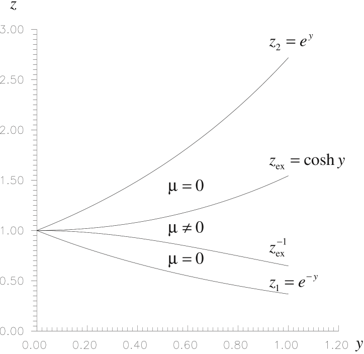
Figure 3: The dependence of specific points of the SF on “time” $y$. It is seen that the region $\mu\neq 0$ vanishes at $y\to 0$. At every moment the solution is a sphere with the centre at $z=\cosh y$ and radius growing as $\sinh y$ ($z_{0}=1$ is accepted).

Comparison to results of the conform transformation for radially stratified medium

Here we compare the results discussed above to the brilliant solution by Korycansky [8] for off-centre explosion in a radially stratified medium. In the Kompaneets approximation the equation $\chi(R,y)=\theta$ for the SF can be written as:

$${\left(\frac{\partial\chi}{\partial y}\right)}^{2}=\frac{1}{\psi(R)}\left[{\left(\frac{\partial\chi}{\partial R}\right)}^{2}+\frac{1}{R^{2}}\right],\quad\psi(R)\equiv\frac{\rho(R)}{\rho_{0}}$$ (42)

Here $R,\theta$ are the spherical coordinates, $R=a,\theta=0,(y=0)$ are the coordinates of the explosion. At $\rho(R)=\rho_{0}(\frac{a}{R})^{n}$, the substitution [8] $\zeta=(\frac{R}{a})^{\alpha}$, $\phi=\alpha\chi$, $\alpha=\frac{2-n}{2}$ leads to the equation in an effective homogeneous medium

$${\left(\frac{\partial\phi}{\partial y}\right)}^{2}=\frac{1}{y_{c}^{2}}\left[{\left(\frac{\partial\phi}{\partial\zeta}\right)}^{2}+\frac{1}{\zeta^{2}}\right],\quad y_{c}=\frac{2a}{|2-n|}.$$ (43)

The solution of [8] is given by the relations:

$$2\zeta\cos\phi=1+\zeta^{2}-x^{2},\quad x\equiv\frac{y}{y_{c}},$$ (44)

$$2\left(\frac{R}{a}\right)^{\frac{2-n}{2}}\cos\frac{(2-n)\theta}{2}=1+\left(\frac{R}{a}\right)^{2-n}-\left[\frac{y(2-n)}{2a}\right]^{2}.$$ (45)

For $n=2$ the following special solution exists [8]:

$$\theta^{2}+\ln^{2}\frac{R}{a}=\left(\frac{y}{a}\right)^{2}.$$ (46)

It can be easily found using the transformation from the spherical case

$${\left(\frac{\partial\chi}{\partial y}\right)}^{2}=\frac{1}{a^{2}}\left[R^{2}{\left(\frac{\partial\chi}{\partial R}\right)}^{2}+1\right]$$ (47)

to the effective plane one with the help of the substitution: $\eta=\ln R$, $y\to ya$:

$${\left(\frac{\partial\chi}{\partial y}\right)}^{2}={\left(\frac{\partial\chi}{\partial\eta}\right)}^{2}+1\Longrightarrow\chi^{2}+\eta^{2}=y^{2}.$$ (48)

The same result can be obtained from the general formula (45) in the limit:

$${{R}{a}^{(2-n)/2}\to\exp\frac{2-n}{2}\ln\frac{R}{a}\to}$$

  (49)

It can be easily verified that main parameters of the surface (46) are very close to that of the sphere discussed above. Correspondence to the case of homogeneous medium can be verified using the transformation to the cylindrical coordinates

$$\left(\frac{\tilde{\rho}}{z}\right)^{2}=\tan^{2}\sqrt{(\frac{y}{z_{0}})^{2}-\ln^{2}\frac{\sqrt{{\tilde{\rho}}^{2}+z^{2}}}{z_{0}}},\quad{\tilde{\rho}}=R\sin\theta,\quad z=R\cos\theta.$$ (50)

At small time

$$\left(\frac{\tilde{\rho}}{z}\right)^{2}=\frac{(y/z_{0})^{2}-\ln^{2}z/z_{0}}{1+\ln z/z_{0}},\quad{\tilde{\rho}}\ll z,z_{0},$$ (51)

it becomes the Sedov solution in ordinary variables:

$${\tilde{\rho}}^{2}+(z-z_{0})^{2}=y^{2}.$$ (52)

Correspondence of solutions for plane-layered and radially stratified media and a new solution for SF in the case of density singularity on the finite radius

The Korycansky transformations can be generalised. The following substitution of variables

$$\frac{z}{z_{0}}=\ln\frac{R}{a}\qquad(R=a\exp\frac{z}{z_{0}})$$ (53)

transforms the Kompaneets equation for $r(z,y)$ in a plane-layered medium (3) (for cylindrical coordinates $z,r$) to that for $\chi(R,y)$ in a radially stratified medium (42) (for spherical coordinates $R,\chi$). This substitution also transforms the density dependence $\varphi(z)$ in a plane-layered medium to $\psi(R)$ in spherical one according to the relation

$$\psi(R)=\varphi(z_{0}\ln\frac{R}{a})\frac{z_{0}^{2}}{R^{2}}$$ (54)

and vice versa:

$$\varphi(z)=\psi(R)\frac{R^{2}}{z_{0}^{2}}=({a}/{z_{0}})^{2}\psi(a\exp\frac{z}{z_{0}})\exp\frac{2z}{z_{0}}.$$ (55)

Corresponding solutions of the Kompaneets equations are related as

$$r=z_{0}\chi.$$ (56)

Note that in this case the exponential density dependencies

$$\varphi(z)=\exp\{-\beta z\}$$ (57)

are transformed to the power ones

$$\psi(R)=\frac{z_{0}^{2}}{R^{2}}\exp\{-\beta z_{0}\ln\frac{R}{a}\}\propto R^{-(\beta z_{0}+2)}.$$ (58)

The equivalent height of the atmosphere for the plane case determines the exponent for the power law in the radially-stratified medium. Particularly, this fact clarifies existence of the solution sequence in the Korycansky case [8], which therefore are connected with Kompaneets solutions [6].

In the special case

$$\varphi(z)\propto 1/z^{2}$$

the exact solution for which is constructed above (see (40)) the law

$$\psi(R)\propto 1/R^{2}\ln^{2}(R/a)$$ (59)

gives the density dependence very close to the inverse-square law at large distances and having a singularity at the surface of the sphere with the radius $a$.

Correspondingly, there is a new formal solution with a fixed point of explosion $R=ae$:

$$\chi(R)=\sqrt{(\ln(R/a)-z_{1}/z_{0})(z_{2}/z_{0}-\ln(R/a))},$$ (60)

where $z_{1,2}(y)/z_{0}$ are defined by the formula (15).

The substitution (53) is also suitable for computations relating to the off-centre explosions in radially stratified media.

Conclusion

The results obtained are in good agreement with the known self-similar solutions [14, 15, 16]. These results can be useful not only for the Solar corona but for another astrophysical situations (compare to [17, 18]) where the inhomogeneity of media is important and, moreover, the inverse-square law of the density decrease occurs very often, for example, for Supernovae in the periphery of gigantic clouds, for outbursts in nebulae [20], for varieties of galactic fountains [21], for galaxies with star formation outbreaks [3] and also for more exotic cases such as the Supernova in the NGC 6946 nearby another Supernova (i.e., in its wind region) [22] recently discovered by the Hubble Space Telescope or for galaxy collisions.

Particularly, the off-centre location of pulsars compared to Supernova Remnants can be naturally explained by displacement of the envelope towards the direction of the density decrease without attracting the idea of the non-symmetrical explosion and recoil. The solution in the medium with the singularity of the density at a sphere surface of a finite radius describes the bypass of the photosphere by the SF and is of great interest for the Sun and stars. The asymptotical solutions for the leading point reveal possible non-monotonic behaviour of the SF velocity at the monotonic density decrease (see [10]). The solutions obtained admits an interesting generalisation if the constant energy $E_{0}$ is replaced by the function of time $E(t)$ which allows to take into account losses [21] as well as an energy supply (see notice in [10]).

Appendix 1

The Kompaneets equation for the SF is derived by equating the normal component of the shock front velocity $D=(p/(\rho-\rho^{2}/\rho^{\prime}))^{1/2}$ obtained from boundary conditions to its formal one $-(\partial f/\partial t)/|\nabla f|$. Here $p=(\gamma-1)\lambda E_{0}/V$ is the pressure behind the shock front, $\gamma$ is the adiabatic exponent, $E_{0}$ is the energy of the explosion, $\rho$ and $\rho^{\prime}$ are densities ahead and behind the shock front, $\rho^{\prime}/\rho=(\gamma+1)/(\gamma-1)$, $V(t)$ is the volume of the envelope $V(t)=\pi\int r^{2}dz$, with the integral taken over the part of $z$ axis, restricted by the envelope. The constant $\lambda$, is of about to 2–3 and accounts the deviation of the pressure near the shock front from the average value, $f(r,z,t)=0$ is the shock front equation.

Appendix 2

Some notes should be made about the leading point behaviour for $\varphi(z)=(z/z_{0})^{-n}$ at $n$ differing from 2. Relations (5), (6) and conditions $r(z_{1,2})=0$ of intersection of axis $z$ by the SF give the following equations for the values $z_{1,2}(y)$:

$$y=\int_{z_{0}}^{z_{2}}dz^{\prime}\Bigl{(}\varphi(z^{\prime})\Bigr{)}^{1/2}=\int_{z_{1}}^{z_{0}}dz^{\prime}\Bigl{(}\varphi(z^{\prime})\Bigr{)}^{1/2}.$$ (61)

In the vicinity of the point $z_{2}$ the value $\xi$ is large and an expansion by $1/\xi\ll 1$ results in the following expression for $\xi^{2}$ [9]:

$$\xi^{2}\approx\left[2\left(z_{2}-z\right)\left(\varphi(z_{2})\right)^{1/2}\right]^{-1}{\int^{z_{2}}_{z_{0}}}du\left(\varphi(u)\right)^{-1/2}$$ (62)

Correspondingly,

$$r\approx(1/\xi(z,y))\cdot{\int^{z}_{z_{0}}}du\left(\varphi(u)\right)^{-1/2},\qquad z\to z_{2}(y).$$ (63)

Thus, the function $\xi$ has a square-root singularity with accordance to (14). These relations can be used to estimate the volume $V(t)$ required to describe motion of the SF in terms of real time $t$. For $z_{2}$ we obtain:

$$z_{2}(t)=\frac{z_{0}}{\left(1-\mathop{\rm sign}\nolimits(n-5)t/t_{*}\right)^{2/(n-5)}},$$ (64)

$$t_{*}=\sqrt{16\pi z_{0}^{5}\rho_{0}/(n+2)(n-5)^{2}E_{0}\lambda(\gamma^{2}-1)}.$$ (65)

As it follows from the relation (61) in the case of $n>5$ [8, 9] “disastrous” acceleration takes place for the mentioned part of the SF which approaches the infinity $z_{2}=\infty$ for a finite time. The expression for the velocity can be written as

$$dz_{2}/dt\propto(t_{*}-t)^{(n-3)/(5-n)}.$$ (66)

The specific time $t_{*}$ of “disastrous” acceleration is

$$t_{*}\approx(z^{5}_{0}\rho_{0}/E_{0})^{1/2}$$ (67)

(see also [9]). Despite the fact that we used here the solution valid only in the vicinity of the leading point the relations (64) and (66) are enough adequate to the phenomena. However, the problem still remains of finding the volume and some features are lost when using such calculations.

References

- [1] Landau L. D., Lifshitz E. M., Fluid Mechanics, 1959, Pergamon Press, London.
- [2] Sedov L. I., 1959, Similarity and Dimansional Methods in Mechanics, Academic Press, New York.
- [3] Bisnovatyi-Kogan G. S., Silich S. A., Revs. Mod. Phys., 1995, V. 67, P. 661.
- [4] Klimishin I. A., 1984, Shock Waves in the Star Envelopes, Nauka, Moskow.
- [5] Hnatyk B. I., Pis’ma Astron.Zh., 1985, V. 11, P. 785.
- [6] Kompaneets A. S., 1960, Dokl. Akad. Nauk SSSR, V. 130, P. 1001 [Sov. Phys. Dokl., 5, 46].
- [7] Silich S. A., Fomin P. I., Dokl. Akad. Nauk SSSR, 1983, V. 268, P. 861 [Sov. Phys. Dokl., 28, 157].
- [8] Korycansky D. G., Astrophys. J., 1992, V. 398, Pt. 1, P. 184.
- [9] Kontorovich V. M., Pimenov S. F., Model of strong explosion in inhomogeneous medium, Dopovidi NAN Ukrainy, 1996, No. 1, P. 54. (In English).
- [10] Kontorovich V. M., Pimenov S. F., Solar Physics, 1997, V. 172, P. 93.
- [11] Kontorovich V. M., Pimenov S. F., Model of strong explosion in a nonuniform corona — from solar radio bursts to relativistic jets, XXVIth Radio Astronomical Conference, Proc., St.-Petersburg, 1995, P. 197.
- [12] Kontorovich V. M., Pimenov S. F., II and IV types radio bursts in the strong explosion model in a nonuniform solar corona, Inform. Bulletin Astron. Ass. Ukraine, 1995, No. 7, P. 93.
- [13] Korn G. A. and Korn T. M., Mathematical Handbook for scientist and engineers, Mc Graw Book Company, N.Y., 1961.
- [14] Parker E. N., Astrophys. J., 1961, V. 133, P. 1014.
- [15] Hundhausen A. J. Coronal Expansion and Solar Wind, 1972, Springer, Heidelberg.
- [16] Sakurai A., Comm. Pure and Appl. Math., 1960. V. 13. P. 353.
- [17] Chernin A. D., Vistas in Astronomy, 1996, V. 40. P. 257.
- [18] Gvaramadze V. V., Pis’ma Astron. Zh., 1997. V. 23, P. 606.
- [19] Muhleman D. O., Anderson J. D., Astrophys. J., 1981, V. 247, P. 1093.
- [20] Lada C. J., Ann. Rev. Astron. Astrophys., 1985, V. 23, P. 267.
- [21] Kovalenko I. G., Shchekinov Yu. A., Astrofizika, 1985, V. 23, P. 363.
- [22] HST News. Supernova collision. http://www.stsci.edu (Usp. Fiz. Nauk, 1997, V. 167, P. 778.)