The D/H ratio at z=0.7 toward Q 1718+4807

Abstract

The apparent discrepancy between low and high D abundances derived from QSO spectra may be caused by spatial correlations in the stochastic velocity field. If one accounts for such correlations, one finds good agreement between different observations and the theoretical predictions for standard big bang nucleosynthesis (SBBN). In particular, we show that the H+D Ly$\alpha$ profile observed at $z_{\rm a}=0.7$ toward Q 1718+4807 is compatible with $4.1\,10^{-5}\;\raise 1.29167pt\hbox{$<$\kern-7.5pt\raise-4.73611pt\hbox{$\sim$}}\;{\rm D/H}\;\raise 1.29167pt\hbox{$<$\kern-7.5pt\raise-4.73611pt\hbox{$\sim$}}\;4.7\,10^{-5}$. This result is consistent with our previous D/H determination for the $z_{\rm a}=2.504$ system toward Q 1009+2956 and, thus, supports SBBN.

1 Introduction

From recent HST observations of a low-redshift ($z_{\rm a}=0.7$) absorption-line system toward the quasar Q 1718+4807 ($z_{e}=1.084$) Webb et al. (1997a,b) deduced D/H = $1.8-3.1\,10^{-4}$. This ratio is significantly higher than that derived from other quasar spectra at $z_{\rm a}=2.504$ [D/H = $1.8-3.5\,10^{-5}$ by Tytler & Burles, 1996; D/H = $2.9-4.6\,10^{-5}$ by Levshakov, Kegel & Takahara, 1997 (LKT, hereinafter)], and at $z_{\rm a}=3.572$ [D/H = $1.7-2.9\,10^{-5}$ by Tytler et al., 1996; D/H $>4\,10^{-5}$ by Songaila et al., 1997].

The apparent spread of the D/H values leads some authors to assume fluctuations in the baryon-to-photon ratio at the epoch of BBN (see e.g. Webb et al., and references cited therein). On the other hand, according to the basic idea of homogeneity and isotropy of big bang theory the primordial deuterium abundance should not vary in space. One can only expect that the D/H ratio decreases with cosmic time due to conversion of D into ³He and heavier elements in stars. To check whether big bang nucleosynthesis has occurred homogeneously or not, precise measurements of absolute values of D/H at high redshift are extremely important. The fundamental character of this cosmological test requires an unambiguous interpretation of spectral observations.

It is well known, however, that the physical parameters derived from spectral data depend on the assumptions made with respect to the line broadening mechanism. For intergalactic absorption lines a ‘non-thermal broadening’ is usually assumed to be caused by large scale motions of the absorbing gas. The commonly used microturbulent approach disregards all correlations of the velocity field, implying a symmetrical (Gaussian) distribution of the velocity components parallel to the line of sight and a symmetrical line profile.

Figure 1: Observations and RMC fits for Q 1718+4807.    a HST/GHRS data (open circles) and calculated profiles for H i (dashed curve), D i (dotted curve) and H+D (solid curve). The latter correspond to model (e) in Table 1. The spectral resolution is 0.1 Å (FWHM). b Residuals $\epsilon$ in units of $\sigma_{\rm noise}$ (see text). c IUE spectrum (open circles) and fit (solid curve). The spectral resolution is 2.95 Å (FWHM)

Actually, any turbulent flow exhibits an immanent structure in which the velocities in neighboring volume elements are correlated with each other. Different aspects of the line formation processes in correlated turbulent media have been discussed recently in a series of papers by Levshakov & Kegel (1997, LK hereinafter), Levshakov, Kegel & Mazets (1997, LKM hereinafter), and by LKT.

Figure 2: As Fig. 1 but for model (c) in Table 1

Once the statistical properties of a turbulent cloud have been specified, the way spectral lines ought to be calculated, depends on the problem considered. Considering emission lines one is dealing with many lines of sight and the observed intensity should closely correspond to the theoretical expectation value (see e.g. Albrecht & Kegel 1987). If, however, one observes the absorption spectrum in the light of a point-like background source, the actually observed line profile is determined by the velocity distribution along the particular line of sight. Therefore, the intensity may deviate substantially from the expectation value, since averaging along one line of sight corresponds to averaging over an incomplete sample (for details see LK and LKM). For large values of the ratio of the cloud thickness $L$ to the correlation length $l$ the distribution function $p(v)$ for the velocity component parallel to the line of sight approaches the statistical average, which has been assumed to be a Gaussian. For values of $L/l$ of only a few, however, $p(v)$ may deviate substantially from a Gaussian, and is asymmetric in general. This leads to a complex shape of the absorption coefficient for which the assumption of Voigt profiles could be extremely misleading. The actual D/H ratio may turn out to be higher or lower than the value obtained from the Voigt-fitting procedure.

The present Letter is primarily aimed at the inverse problem in the analysis of the H+D Ly$\alpha$ absorption observed by Webb et al. (1997a,b). The original analysis was performed in the framework of the microturbulent model. Here we make an attempt to re-analyze the observational data on the basis of a more general mesoturbulent model. We consider a cloud with a stochastic velocity field with finite correlation length but of homogeneous (H i-) density and temperature. The velocity field is characterized by its rms amplitude $\sigma_{\rm t}$ and its correlation length $l$. The model is identical to that of LKT. – The objective is to investigate whether the data in question may also be interpreted by a lower D/H ratio consistent with the values found for other absorption systems.

2 Parameter estimation

To estimate physical parameters and an appropriate velocity field structure along the line of sight, we used a Reverse Monte Carlo [RMC] technique (see LKT). The algorithm requires to define a simulation box for the 5 physical parameters : N(H i), D/H, $T_{\rm kin}$, $\sigma_{\rm t}/v_{\rm th}$, and $L/l$ (here $v_{\rm th}$ denotes the thermal width of the hydrogen lines). – The continuous random function of the coordinate $v(s)$ is represented by its sampled values at equal space intervals $\Delta s$, i.e. by $\{v_{1},v_{2},\dots,v_{k}\}$, the vector of the velocity components parallel to the line of sight at the spatial points $s_{j}$.

Figure 3: Probability density functions (p.d.f.) for residuals $\epsilon$ shown by dotted line (corresponds to Fig.1b) and by solid line (corresponds to Fig.2b) and their fit by a Gaussian with mean $E(\epsilon)=0$ and variance $Var(\epsilon)=1$

In the present study we adopted for the physical parameters the following boundaries :

According to Webb et al., N(H i) is well restricted within the range from 1.70$\,10^{17}$ cm^-2 to 1.78$\,10^{17}$ cm^-2, as derived from the observed Lyman-limit discontinuity.

For D/H we use the range from 3.0$\,10^{-5}$ to 5.0$\,10^{-5}$, trying to find a low D/H solution.

To restrict $T_{\rm kin}$ and $\sigma_{\rm t}/v_{\rm th}$ one has to assume a model for the absorbing material. It is generally believed that absorption line systems with N(H i) $\sim 10^{17}$ cm^-2 arise in the halos of putative intervening galaxies. Direct observations of galactic halos at $z>2$ (van Ojik et al. 1997) show that $\sigma_{\rm t}\simeq 40\pm 15$ km s^-1, if $T_{\rm kin}\simeq 10^{4}$ K. For $T_{\rm kin}$ we use the interval $10^{4}-2\,10^{4}$ K, and, thus, $\sigma_{\rm t}/v_{\rm th}$ may range within 1.3 – 4.3 .

For $L/l\gg 1$ the meso- and microturbulent profiles tend to be identical (see LK). Webb et al. thoroughly investigated different microturbulent models. Therefore we consider only moderate $L/l$ ratios in the range 1.0 – 5.0.

Following Webb et al. (1997b), we exclude the Si iii line from our analysis of the H+D Ly$\alpha$ profile. As shown by Vidal-Madjar et al. (1996), ‘deducting lines of sight velocity structure for D/H evaluations from ionized species could be extremely misleading’. But we fix $z_{\rm a}$(Si iii) = 0.701024 as a more or less arbitrary reference radial velocity at which $v_{j}=0$.

Having specified the parameter space, we construct the objective function (LKT) :

$${\cal L}\equiv\chi^{2}=\frac{1}{\nu}\sum^{m}_{i=1}\left[\frac{I(\lambda_{i})-r(\lambda_{i})}{\sigma_{\rm noise}}\right]^{2}\,,$$ (1)

where $r(\lambda_{i})$ is the simulated random intensity, $I(\lambda_{i})$ the observed normalized intensity within the $i$th pixel of the line profile, $\sigma_{\rm noise}$ the experimental error level, and $\nu=m-n$   the degree of freedom ($m$ is the number of data points and $n$ is the number of fitted physical parameters, $n=5$ in our case).

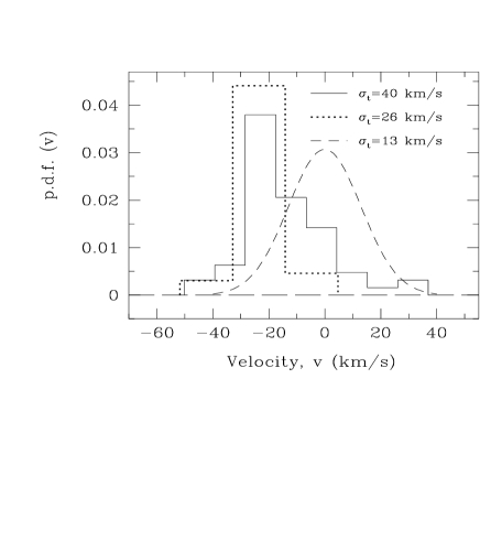
Figure 4: Probability density functions (p.d.f.) for velocity components $p(v)$ for the RMC solutions shown in Fig.1a (dotted line histogram) and in Fig.2a (solid line histogram). Both are blue-shifted by about $-20$ km s^-1 with respect to $z_{\rm a}$(Si iii). Note the asymmetric shapes. For comparison, the short dashed line shows $p(v)$ for the microturbulent model adopted by Webb et al.

Here $\sigma_{\rm noise}$ is assumed to be constant over the entire H+D profile. In order to estimate $\sigma_{\rm noise}$ we have chosen a portion of the Q 1718+4807 continuum from the left ($\Delta\lambda_{\rm L}=2066.02-2066.90$ Å) and the right ($\Delta\lambda_{\rm R}=2068.52-2070.01$ Å) hand side of the hydrogen absorption (see Fig. 1), as well as the bottom of the Ly$\alpha$ line ($\Delta\lambda_{\rm B}=2067.35-2068.30$ Å). These three regions yield $\sigma_{\rm L}=0.095$, $\sigma_{\rm R}=0.093$, and $\sigma_{\rm B}=0.086$, respectively. At $z=0.7$ where the number density of the Ly$\alpha$ lines is far lower than at high redshifts, the experimental noise is expected to be free from the contamination by weak Ly$\alpha$ forest lines. Therefore the estimated noise level corresponds to the experimental uncertainties. To approximate the error level we set $\sigma_{\rm noise}=0.09$.

Finally, our objective function contains only the blue and the red wing of the H i line ($\Delta\lambda=2066.90-2067.35$ Å and $\Delta\lambda=2068.30-2068.52$ Å, respectively) since they are more sensitive to the parameter variations than the central part of the line is. By this we restrict the total number of data points to $m=30$, implying $\nu=25$ and $\frac{1}{\nu}\chi^{2}_{\nu,\alpha}=1.174$ for the credible probability $P_{\alpha}=1-\alpha=0.75$.

The estimated parameters for a few adequate RMC profile fits ($\chi^{2}_{\rm min}<\chi^{2}_{25,0.25}$) are listed in Table 1. The derived deuterium abundance $\langle{\rm D/H}\rangle\simeq 4.4\,10^{-5}$ is about 4–7 times smaller than the limiting values of $1.8-3.1\,10^{-4}$ found by Webb et al. (1997b) in the microturbulent model excluding the Si iii line. To illustrate our results, we show in Figs. 1 and 2 H+D Ly$\alpha$ profiles for the two calculations with the lowest and the highest D abundances found in the mesoturbulent model (D/H = $4.111\,10^{-5}$ and $4.755\,10^{-5}$, respectively). They are shown by the solid curve, whereas the open circles give the experimental intensities $I(\lambda_{i})$.

The residuals $\epsilon_{i}=[I(\lambda_{i})-r(\lambda_{i})]/\sigma_{\rm noise}$ shown in Figs. 1b and 2b by filled circles are normally distributed with zero mean and unit variance (see Fig. 3). This fact, rather trivial in case of high S/N data, becomes crucial when dealing with spectra as noisy as the present one is, because of the probability to be trapped into fitting the noise features. The good concordance of the residuals with the expected normal distribution is here a significant argument for the validity of the results obtained.

Table 1: Cloud parameters derived from the Ly$\alpha$ profile by the RMC method [${\rm N}_{17}$(H i) column density in units of $10^{17}$ cm^-2, D/H in units of $10^{-5}$, $T_{4,\rm kin}$ kinetic temperature in units of $10^{4}$ K, $\sigma_{t}$ turbulent velocity in km s^-1]

	N17(H i)	D/H	$T_{4,\rm kin}$	$\sigma_{t}$	$L/l$	$\frac{1}{\nu}\chi^{2}_{\rm min}$
(a)	1.732	4.565	1.41	22	2.7	1.064
(b)	1.739	4.562	1.60	18	3.9	1.002
(c)	1.759	4.755	1.75	40	2.8	1.106
(d)	1.761	4.555	1.46	29	4.3	1.086
(e)	1.768	4.111	1.51	26	3.5	0.897
(f)	1.771	4.442	1.76	23	3.4	1.162
(g)	1.776	4.249	1.62	28	4.0	1.114

To check the $v(s)$-configurations estimated by the RMC procedure, we calculated profiles for the higher order Lyman lines and the shape of the Lyman-limit discontinuity and then superposed them to the corresponding part of the IUE spectrum. The results are shown in Figs. 1c and 2c where again open circles correspond to the observed intensities and the computed spectra are shown by the solid curves. We do not find any pronounced discordance of calculated and real spectra. On the other hand, the spectral resolution of 2.95 Å is not sufficient to follow a fine velocity field structure within the $z_{\rm a}=0.7$ absorber.

The derived $v(s)$-configurations are not unique. Table 1 demonstrates the spread of the rms turbulent velocities from 18 up to 40 km s^-1. It is worthwhile to emphasize once more that the projected velocity distribution function may differ considerably from a Gaussian. Fig. 4 shows an example of such distortions caused by a poor statistical sample (i.e. incomplete averaging) of the velocity field distributions for the two cases of the lowest and the highest D/H ratios from Table 1 [model (e) and (c), respectively]. Both $p(v)$ distributions are asymmetric. This is the main reason why the absorption in the blue wing of the H i Ly$\alpha$ line may be enhanced without any additional H i interloper(s).

3 Conclusion

Figure 5: The H i Ly-4 and Ly-12 mesoturbulent spectra for model (c) (solid curves) and (e) (dotted curves) in Table 1. Short dashed curves show microturbulent profiles calculated for the mean N(H i) = $1.738\,10^{17}$ cm^-1 and the mean Doppler parameter $b$(H i) = 25.5 km s^-1 of the data by Webb et al. The spectra are convolved with a Gaussian instrumental profile of FWHM = 0.1 Å 

We have shown that the interpretation of the HST and IUE spectra obtained by Webb et al. is not unique. The data can as well be modeled with a low value of the D/H ratio if one accounts for spatial correlations in the large scale velocity field.

The RMC results may be tested, in principle, by additional observations of higher order Lyman lines with the same spectral resolution as Webb et al. used for Ly-$\alpha$. Indeed, if $p(v)$ is asymmetric, this will show up in the profile shapes of the higher order Lyman lines. For the physical parameters listed in Table 1, the effect becomes visible starting from Ly-4 [the Ly-$\alpha$, -$\beta$, -$\gamma$ lines are insensitive to the asymmetry of $p(v)$ due to their high optical depth]. Fig. 5 shows simulated spectra (convolved with a Gaussian instrumental profile of FWHM = 0.1 Å) for Ly-4 and Ly-12 using the same $p(v)$ distributions depicted in Fig. 4 – dotted curves for model (e) and solid curves for model (c) of Table 1. The line shapes clearly depend on the velocity field structure and are asymmetric in general.