Testing Cold Dark Matter Models Using Hubble Flow Variations

Abstract

COBE-normalized flat (matter plus cosmological constant) and open Cold Dark Matter (CDM) models are tested by comparing their expected Hubble flow variations and the observed variations in a Type Ia supernova sample and a Tully Fisher cluster sample. The test provides a probe of the CDM power spectrum on scales of $0.02h$ Mpc${}^{-1}\la k\la 0.2h$ Mpc^-1, free of the bias factor $b$. The results favor a low matter content universe, or a flat matter-dominated universe with a very low Hubble constant and/or a very small spectral index $n_{\rm ps}$, with the best fits having $\Omega_{0}\sim 0.3$ to 0.4. The test is found to be more discriminative to the open CDM models than to the flat CDM models. For example, the test results are found to be compatible with those from the X-ray cluster abundance measurements at smaller length scales, and consistent with the galaxy and cluster correlation analysis of Peacock and Dodds (1994) at similar length scales, if our universe is flat; but the results are marginally incompatible with the X-ray cluster abundance measurements if our universe is open. The open CDM results are consistent with that of Peacock and Dodds only if the matter density of the universe is less than about 60% of the critical density. The shortcoming of the test is discussed, so are ways to minimize it.

1 Introduction

In a previous paper on Hubble flow variations (Shi 1997a), I calculated the limit on the power spectrum shape parameter $\Gamma$ for flat CDM models. In this paper I extend the test of Hubble flow variations to open CDM models, and do a likelihood analysis of both type of models. Furthermore, I will compare the results to those from other methods that test the CDM power spectrum. Finally, I will discuss the major shortcoming of this test, and possible improvements that can be made to minimize it.

Before going into details, I would like to point out first that the method outlined here is different from that of Jaffe and Kaiser (1995). In Jaffe and Kaiser (1995), multi-mode deviations from a pure Hubble expansion, including the bulk motion and shears were investigated for samples as a whole. In the method presented here, the variations of the Hubble expansion, corresponding to the isotropic component of Jaffe and Kaiser’s multi-mode deviation, are investigated within samples for every subsample (excluding those with too small sizes such that non-linearity becomes an issue). Therefore the Hubble flow variation method is sensitive to the scale dependence and the shape of the variations, while the method of Jaffe and Kaiser is not. The two methods are however based on the same theoretical premise: density fluctuations give rise to peculiar velocities through gravity, and therefore from the amplitude and direction of peculiar velocity fields one can infer the underlying density fluctuations. It will be interesting to combine the two methods, by testing the variations of all modes of peculiar velocities, though it will be significantly more cpu intensive.

The formalism of testing models using Hubble flow variations has been reviewed in Shi (1997a,b). Here a summarization suffices. The deviation from a global Hubble expansion rate $H_{0}$, $\delta H$ ($=H_{\rm Local}-H_{0}$), of a sample is

$$\delta H=B^{-1}\sum_{q}{S_{q}r_{q}-U_{i}r_{q}\hat{r}_{q}^{i}\over\sigma_{q}^{2}},$$ (1)

where its bulk motion is

$$U_{i}=(A-RB^{-1})^{-1}_{ij}\Bigl{(}\sum_{q}{S_{q}{\hat{r}}_{q}^{j}\over\sigma_{q}^{2}}-B^{-1}\sum_{q}\sum_{q^{\prime}}{S_{q}r_{q}r_{q^{\prime}}{\hat{r}}_{q^{\prime}}^{j}\over\sigma_{q}^{2}\sigma_{q^{\prime}}^{2}}\Bigr{)},$$ (2)

and

$$A_{ij}=\sum_{q}{\hat{r}_{q}^{i}\hat{r}_{q}^{j}\over\sigma_{q}^{2}},\,\,R_{ij}=\sum_{q}\sum_{q^{\prime}}{r_{q}\hat{r}_{q}^{i}r_{q^{\prime}}\hat{r}_{q^{\prime}}^{j}\over\sigma_{q}^{2}\sigma_{q^{\prime}}^{2}},\,\,B=\sum_{q}{r_{q}^{2}\over\sigma_{q}^{2}}.$$ (3)

In the equations, ${\bf r}_{q}$ is the position of object $q$ in the sample (with earth at the origin), and $S_{q}$ ($=cz_{q}-H_{0}r_{q}$) is its estimated line-of-sight peculiar velocity with an uncertainty $\sigma_{q}$. Spatial indices $i,j$ run from $1,2,3$, and identical indices indicate summation.

Formally $\delta H$ can always be expressed in the form

$$\delta H=\int{\rm d}^{3}r\,\tilde{W}({\bf r})\,S({\bf r}),$$ (4)

where $\tilde{W}({\bf r})$ is the window function of the $\delta H$ measurement, and $S({\bf r})$ is the estimated line-of-sight peculiar velocity field. It is not hard to see from eqs. (1), (2) and (3) that

$$\tilde{W}({\bf r}) = B^{-1}\Bigl{\{}\sum_{q}{r_{q}\over\sigma_{q}^{2}}\delta({\bf r}-{\bf r}_{q})-$$ (5)

$$(A-RB^{-1})^{-1}_{jl}\Bigl{[}\sum_{q}{\hat{r}_{q}^{j}\over\sigma_{q}^{2}}\delta({\bf r}-{\bf r}_{q})-$$

$$B^{-1}\sum_{q}\sum_{q^{\prime}}{r_{q}r_{q^{\prime}}^{j}\over\sigma_{q}^{2}\sigma_{q^{\prime}}^{2}}\delta({\bf r}-{\bf r}_{q})\Bigr{]}\sum_{q^{\prime\prime}}{r_{q^{\prime\prime}}^{l}\over\sigma_{q^{\prime\prime}}^{2}}\Bigr{\}}.$$

If most of the uncertainty in $S_{q}$ comes from the uncertainty in measuring the distance $r_{q}$, which is true at scales beyond $\sim 5000$ km/sec, then $\sigma_{q}\propto r_{q}$. As a result, the window function $\tilde{W}$ scales linearly with $H_{0}$.

The estimated line-of-sight peculiar velocity of object $q$, $S_{q}$, is related to its true peculiar velocity ${\bf v}({\bf r_{q}})$ by

$$S_{q}=v_{i}({\bf r}_{q})\hat{r}^{i}_{q}+\epsilon_{q},$$ (6)

where $\epsilon_{q}$ is the uncertainty of the estimate with the standard deviation of $\sigma_{q}$. Therefore, $\delta H$ can be broken into two parts: the true deviation $\delta H^{(v)}$ and the noise $\delta H^{(\epsilon)}$. Eq. (4) then becomes

$$\delta H=\delta H^{(v)}+\delta H^{(\epsilon)}=\int{\rm d}^{3}r\,W^{i}({\bf r})\,v_{i}({\bf r})\,+\,\int{\rm d}^{3}r\,\tilde{W}({\bf r})\,\epsilon,$$ (7)

where $W^{i}({\bf r})=\tilde{W}({\bf r})\,\hat{r}^{i}$. The variance of $\delta H^{(v)}$ depends on the density power spectrum of our universe $P(k)$, the matter content of our universe $\Omega_{0}$ (the matter density divided by the critical density), and the global Hubble constant $H_{0}$, in the following way (Shi 1997a,b):

$$\bigl{\langle}\bigl{(}\delta H^{(v)}\bigr{)}^{2}\bigr{\rangle}=H_{0}^{2}\,\Omega_{0}^{1.2}\int{\rm d}^{3}k\bigl{|}W^{i}({\bf k})\hat{k}_{i}\bigr{|}^{2}{P(k)\over k^{2}},$$ (8)

where the Fourier transform of $W^{i}({\bf r})$, $W^{i}({\bf k})$, is

$$W^{i}({\bf k}) = {B^{-1}\over(2\pi)^{3/2}}\Bigl{[}\sum_{q}{r_{q}^{i}\over\sigma_{q}^{2}}e^{i{\bf k}\cdot{\bf r}_{q}}$$ (9)

$$- (A-RB^{-1})^{-1}_{jl}\Bigl{(}\sum_{q}{\hat{r}_{q}^{i}\hat{r}_{q}^{j}\over\sigma_{q}^{2}}e^{i{\bf k}\cdot{\bf r}_{q}}$$

$$- B^{-1}\sum_{q}\sum_{q^{\prime}}{r_{q}^{i}r_{q^{\prime}}^{j}\over\sigma_{q}^{2}\sigma_{q^{\prime}}^{2}}e^{i{\bf k}\cdot{\bf r}_{q}}\Bigr{)}\sum_{q^{\prime\prime}}{r_{q^{\prime\prime}}^{l}\over\sigma_{q^{\prime\prime}}^{2}}\Bigr{]}.$$

The variance of $\delta H^{(\epsilon)}$ depends on the sample measures and $H_{0}$ in the following form:

$$\bigl{\langle}\bigl{(}\delta H^{(\epsilon)}\bigr{)}^{2}\bigr{\rangle}=H_{0}^{2}\bigl{(}B^{-1}+B^{-2}(A-RB^{-1})^{-1}_{il}R_{il}\bigr{)}.$$ (10)

If the value of $H_{0}$ is precisely known, the above variances can be directly calculated for a sample, and be compared with the observed deviations. But the value of $H_{0}$ is still controversial, which leaves us the only option of investigating the relative variation of Hubble flows within a sample. In other words, if the expansion rate of a sample with $N$ objects is $H_{N}$, and the expansion rate of a subsample with $n$ ($<N$) objects is $H_{n}$, a comparison can be made between the variation $\delta H_{nN}/H_{N}=(H_{n}-H_{N})/H_{N}$ and its theoretical expectation without knowing the absolute value of $H_{0}$. Under the condition that $H_{N}\approx H_{0}$ (i.e., $\langle(H_{N}-H_{0})^{2}/H_{0}^{2}\rangle^{1/2}\ll 1$), the variance of $\delta H_{nN}/H_{N}$ is

$$\Bigl{\langle}\Bigl{(}{\delta H_{nN}\over H_{N}}\Bigr{)}^{2}\Bigr{\rangle}$$ (11)

$$\approx \Bigl{\langle}\Bigl{(}{\delta H_{n}^{(v)}\over H_{0}}\Bigr{)}^{2}+\Bigl{(}{\delta H_{N}^{(v)}\over H_{0}}\Bigr{)}^{2}-2\Bigl{(}{\delta H_{n}^{(v)}\over H_{0}}\Bigr{)}\Bigl{(}{\delta H_{N}^{(v)}\over H_{0}}\Bigr{)}\Bigr{\rangle}$$

$$+ \Bigl{\langle}\Bigl{(}{\delta H_{n}^{(\epsilon)}\over H_{0}}\Bigr{)}^{2}+\Bigl{(}{\delta H_{N}^{(\epsilon)}\over H_{0}}\Bigr{)}^{2}-2\Bigl{(}{\delta H_{n}^{(\epsilon)}\over H_{0}}\Bigr{)}\Bigl{(}{\delta H_{N}^{(\epsilon)}\over H_{0}}\Bigr{)}\Bigr{\rangle},$$

where variances of $\delta H_{n}$ and $\delta H_{N}$ are calculated through eqs. (8) and (10) using their respective window functions $W^{i}_{n}({\bf k})$ and $W^{i}_{N}({\bf k})$. The cross correlation of the expected variations is

$$\Bigl{\langle}\Bigl{(}{\delta H_{n}^{(v)}\over H_{0}}\Bigr{)}\Bigl{(}{\delta H_{N}^{(v)}\over H_{0}}\Bigr{)}\Bigr{\rangle}$$ (12)

$$= \Omega_{0}^{1.2}\int{\rm d}^{3}k\,{\rm Re}\bigl{[}W^{i}_{n}({\bf k})\hat{k}_{i}{W^{j}_{N}}^{*}({\bf k})\hat{k}_{j}\bigr{]}\,{P(k)\over k^{2}},$$

where Re[…] denotes the real part of the argument, and $*$ denotes complex conjugation. The correlation of the noises is

$$\Bigl{\langle}\Bigl{(}{\delta H_{n}^{(\epsilon)}\over H_{0}}\Bigr{)}\Bigl{(}{\delta H_{N}^{(\epsilon)}\over H_{0}}\Bigr{)}\Bigr{\rangle}=\Bigl{\langle}\Bigl{(}{\delta H_{N}^{(\epsilon)}\over H_{0}}\Bigr{)}^{2}\Bigr{\rangle}.$$ (13)

The size of the samples I discuss in this paper is sufficiently large that their cosmic+sampling variance $\langle(\delta H_{N}/H_{0})^{2}\rangle^{1/2}$ is less than 3 percent (Shi & Turner 1998). Eq. (11) is therefore a very good approximation. The calculation of the variation $\delta_{nN}$ and its variance, on the other hand, has taken full account of both cosmic variance and sampling variance. They therefore do not depend on the sampling size of the (sub)sample. Of course for a small size subsample with too few objects, the variance of $\delta H_{nN}$ becomes large, so that a comparison between observations and the theoretical expectation will yield a less significant result. But the result is still statistically sound.

Figure 1: Hubble flow variations (with 1$\sigma$ errorbars) vs. the depth of subsamples of the Type Ia SN sample. Curves are noise-free 1$\sigma$ expectation from three models.

Figure 2: The same as fig. 1 but for the TF cluster sample.

In figures 1 and 2 I plot the Hubble flow variation $\delta H_{nN}$, compared with the noise-free model expectation of the standard deviation $\langle(\delta H_{nN}/H_{N})^{2}\rangle^{1/2}$, as a function of the maximal depth $R$ of subsamples (defined to include $n$ most nearby objects), for a sample of 20 Type Ia supernovae (SNe) (Riess et al. 1996) and a sample of 36 clusters with Tully-Fisher (TF) distances (Willick et al. 1997), respectively. Three representative models are chosen for comparison: (1) the standard CDM model (sCDM), with $\Omega_{0}=1$, $h\equiv H_{0}/(100{\rm km/sec/Mpc})=0.5$ and the power spectrum index $n_{\rm ps}=1$; (2) the tilted CDM model (tCDM), with $\Omega_{0}=1$, $h=0.5$ and $n_{\rm ps}=0.7$; (3) the vacuum energy $\Lambda$ dominated flat CDM model ($\Lambda$CDM), with $\Lambda=0.7$, $\Omega_{0}=0.3$, $h=0.7$, and $n_{\rm ps}=1$. The power spectra of these models have the same functional form and COBE-normalization as in Shi (1997a). The Type Ia SN sample does not show significant detection of Hubble flow variations. It therefore favors models with smaller power on $\sim 40h^{-1}$ to 200$h^{-1}$ Mpc scales, because otherwise its Hubble flow variation would be significantly larger. The TF cluster sample shows a significant detection of Hubble flow variations on 45$h^{-1}$ to 60$h^{-1}$ Mpc scale. Its implication on models, however, is not obvious.

To quantify the implications of figs. 1 and 2, a likelihood analysis is needed. Since different subsamples are not independent, we need to know the expected correlation between the Hubble flow variations of two different subsamples, $\delta H_{nN}$ and $\delta H_{mN}$ ($m\leq n$). This correlation is

$$\Sigma_{nm} = \Bigl{\langle}\Bigl{(}{\delta H_{nN}\over H_{N}}\Bigr{)}\Bigl{(}{\delta H_{mN}\over H_{N}}\Bigr{)}\Bigr{\rangle}$$ (14)

$$\approx \Omega_{0}^{1.2}\int{\rm d}^{3}k\,{\rm Re}\Bigl{\{}\Bigl{[}W^{i}_{n}({\bf k})-W^{i}_{N}({\bf k})\Bigr{]}\hat{k}_{i}\times$$

$$\Bigl{[}{W^{j}_{m}}^{*}({\bf k})-{W^{j}_{N}}^{*}({\bf k})\Bigr{]}\hat{k}_{j}\Bigr{\}}\,{P(k)\over k^{2}}$$

$$+ \Bigl{\langle}\Bigl{(}{\delta H_{n}^{(\epsilon)}\over H_{0}}\Bigr{)}^{2}-\Bigl{(}{\delta H_{N}^{(\epsilon)}\over H_{0}}\Bigr{)}^{2}\Bigr{\rangle}.$$

Given vector $(\Delta H)_{n}=\delta H_{nN}$ ($n=n_{\rm min},n_{\rm min}+1,...,N-1$) measured from a real sample $D$, the likelihood of a cosmological model with a set of parameters $\theta$ is

$$P\langle\theta|DI\rangle={1\over{\cal N}|\Sigma|^{1/2}}\exp\Big{[}-{1\over 2}({\Delta H})^{T}(\Sigma)^{-1}(\Delta H)\Bigr{]},$$ (15)

with a normalization

$${\cal N}=\int{\rm d}\theta{1\over|\Sigma|^{1/2}}\exp\Big{[}-{1\over 2}({\Delta H})^{T}(\Sigma)^{-1}(\Delta H)\Bigr{]}.$$ (16)

I test $\delta H_{nN}$ here instead of $H_{n}-H_{n-1}$ as in Shi (1997a), because no advantage was found using the latter quantity. The statistical tests of the two quantities, however, are almost equivalent and give similar results.

2 Results and Discussions

I apply eqs. (1) to (16) to two sets of COBE-normalized CDM models, the open CDM models ($\Omega_{0}<1$ and $\Lambda=0$) and the flat $\Lambda$CDM models ($\Omega_{0}+\Lambda=1$). The parameters of the models are chosen to be $\Omega_{0}$, $h$ and $n_{\rm ps}$. For open (flat) CDM models, I choose the prior distribution of the parameters to be $0.2<\Omega_{0}<1$ ($0.3<\Omega_{0}<1$), $0.5<h<0.8$ and $0.7<n_{\rm ps}<1.2$, with uniformly distributed likelihood. The ranges of parameters are chosen conservatively to reflect measurements of mass densities on the galaxy cluster scale (Carlberg, Yee and Ellingson 1997), quasar lensing statistics in the case of flat CDM models (Kochanek 1996), Cosmic Microwave Background (Lineweaver and Barbosa 1997) and the Hubble constant (Freedman 1997). The final likelihood distribution functions after taking into account Hubble flow variations are then calculated according to eq. (15), with $\theta$ being a three dimensional parameter space $(\Omega_{0},h,n_{\rm ps})$. Figures 3–6 show on slices of constant $n_{\rm ps}$ the 68$\%$ and $95\%$ C.L. contours in the 3-D parameter space, for open CDM models and flat CDM models, using the Type Ia SN sample and TF cluster sample. Only subsamples with a depth of more than $40h^{-1}$ Mpc are used to ensure the validity of linear perturbation theory of gravity.

Figures 3 to 6 clearly show that models with smaller powers are favored by both samples. Models with $\Omega_{0}\sim$0.3 to 0.4 fit data quite well regardless of the choice of $h$, $n_{\rm ps}$ or the geometry of the universe. $\Omega_{0}=1$ models, on the other hand, are strongly disfavored unless $n_{\rm ps}$ and $h$ approach the lower end of their allowed ranges. The result diverges from a previous belief that peculiar velocity fields favor a high matter density universe. The figures also show that the Hubble variation method is a more discriminative test to COBE-normalized open models.

Figure 3: The 68$\%$ (the dashed line) and $95\%$ (the solid line) C.L. contours in the $(\Omega_{0},h,n_{\rm ps})$ parameter space on different $n_{\rm ps}={\rm constant}$ slices, for open CDM models using the Type Ia SN sample. Areas to the left of the contours are allowed at their corresponding confidence levels. Shaded regions are allowed at the 2$\sigma$ level by the X-ray cluster temperature function. The cross denotes the best fit. (a) $n_{\rm ps}=0.725$; (b) $n_{\rm ps}=0.875$; (b) $n_{\rm ps}=1.025$; (b) $n_{\rm ps}=1.175$.

Figure 4: The same as fig. 3 but using the TF cluster sample. Areas sandwiched between two dashed lines are allowed at 68% C.L. Areas to left of the solid line are allowed at 95% C.L.

Figure 5: The same as fig. 3 but for flat $\Lambda$CDM models.

Figure 6: The same as fig. 3 but for flat $\Lambda$CDM models using the TF cluster sample.

Also plotted in the figures is the parameter space allowed by the X-ray cluster temperature function constraint, $\sigma_{8}\Omega_{0}^{\alpha}=0.52\pm 0.04$ with $\alpha=0.52-0.13\Omega_{0}$ for $\Lambda$CDM and $\alpha=0.46-0.10\Omega_{0}$ for open CDM (Eke et al. 1996; see also similar results of Viana and Liddle 1996, and Pen 1996), at the 2$\sigma$ level, if its error is taken at a face value. Since the X-ray cluster temperature function probes the power spectrum on $\sim 8h^{-1}$ Mpc scale, while Hubble flow variation calculation probes mainly scales from $\sim 30h^{-1}$ to $\sim 200h^{-1}$ Mpc (as shown in figure 7), their consistency is not automatically guaranteed. Figures 3 to 6 show that the two methodologies do give consistent results for individual samples.

Figure 7: The window function vs. its scale. (a) the TF cluster subsamples with $n=15$ (the solid line) and $n=N-1=35$ (the dashed line, multiplied by 100); (b) the Type Ia SN subsamples with $n=8$ (the solid line) and $n=N-1=19$ (the dashed line, multiplied by 10). Only one direction of ${\bf k}$ is shown. The plotted function looks similar in other ${\bf k}$ directions.

When both samples are used to calculate a joint likelihood of models, models with smaller powers are more strongly favored, as seen in figure 8 and 9. However, while figure 9 shows that the Hubble flow result is still compatible with the X-ray cluster constraints in the COBE-normalized $\Lambda$CDM models, figure 8 indicates that the two are marginally incompatible in the COBE-normalized open CDM models. Does it hint that the flat universe with a vacuum energy is a more likely scenario for our universe? It is probably premature to say so, because the inconsistency is only marginal. At this stage, it may tell us more about the smoother distribution of the likelihood in $\Lambda$CDM models relative to open CDM models, than about the favoring of one class of models against the other. If, however, the gap between the Hubble variation result and the X-ray cluster result widens in open CDM models in the future, we may need to seriously consider its cosmological implications.

Figure 8: The joint likelihood distribution using both samples, for open CDM models. Legends are the same as in figure 3 to 6.

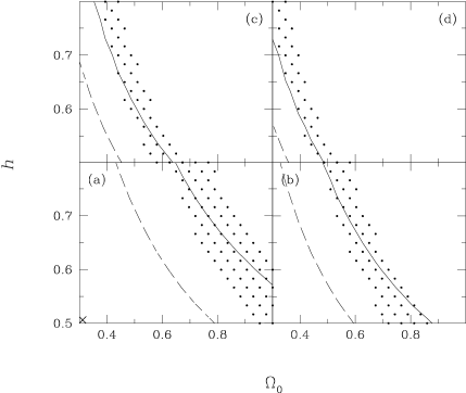
Figure 9: The joint likelihood distribution using both samples, for flat $\Lambda$CDM models. Legends are the same as in figure 3 to 6.

It is also interesting to compare the Hubble variation result to the power spectrum inferred from the galaxy and cluster correlation analysis of Peacock and Dodds (1994). Since the two approaches both test $\sim 100h^{-1}$ Mpc scales, certain consistency is expected. Figure 10(a) plots $\Omega_{0}^{1.2}P(k)$ (which the Hubble flow variation truely measures) of a number of open CDM models along the 95$\%$ C.L. contour in fig. 8. Since these models are marginally allowed at 95$\%$ C.L., the upper envelope of their $\Omega_{0}^{1.2}P(k)$ curves in the tested range of $0.02\,{\rm Mpc}^{-1}\la k/h\la 0.2\,{\rm Mpc}^{-1}$ represents a reasonable upper limit to $\Omega_{0}^{1.2}P(k)$ of the COBE-normalized open CDM models. A similar limit can also be obtained for the COBE-normalized $\Lambda$CDM models. Figure 10(b) shows that this upper limit for the COBE-normalized open CDM models is lower than the $\Omega_{0}^{1.2}P(k)$ of Peacock and Dodds (1994), had our universe had $\Omega_{0}$ approaching 1. This upper limit is consistent with Peacock and Dodds’ result only if the universe has $\Omega_{0}\la 0.6$, given the $\Omega_{0}^{-0.3}$ dependence of their deduced $P(k)$. For $\Lambda$CDM models, the upper limit on $\Omega_{0}^{1.2}P(k)$ is consistent with the result of Peacock and Dodds even if $\Omega_{0}=1$, although the consistency at $\Omega_{0}=1$ is marginal. The comparison once again shows that small $\Omega_{0}$ is favored, and that the test of Hubble flow variation is more discriminative to the COBE-normalized open CDM models than to the COBE-normalized $\Lambda$CDM models.

One major shortcoming of the Hubble flow variation test is that the likelihood distribution is not symmetric relative to the peak probability (figs. 3 to 6 and figs. 8 and 9) so that it has less power discriminating against models predicting too small Hubble flow variations than against models with too large Hubble flow variations. This is due to the fact that the noise term in eq. (14) dominates the Hubble flow variation when the true density fluctuations are small. Thus the key to increase the testing power on models with small $P(k)$ (and on models with larger $P(k)$ to a lesser degree), is to reduce the noise term with better distance measurements, and more objects in the same sample volume. Since the observed and expected $\delta H_{nN}/H_{N}$ is typically a few percent at a depth of $\la 5,000$ to 10,000 km/sec, the noise contribution to $\delta H_{nN}/H_{N}$ has to be $\la 1\%$ to ensure a significant detection of $\delta H_{nN}/H_{N}$ and a little skewed likelihood distribution. For Type Ia SN samples, where distance measurement errors are typically 5$\%$ and random motions due to local non-linearities contribute $\sim 5\%$ of recession velocities at $\la 10,000$ km/sec, the number of Type Ia SNe has to be $\ga 50$ within $\sim 10,000$ km/sec to reduce the noise term to $\la 1\%$. Apparently the sample used here (with the number around 15) is not enough (as shown by the one-sided likelihood distribution in figs. 3 and 5). But as the number of Type Ia SNe observed increases rapidly (for instance, there are 25 Type Ia SNe below 10,000 km/sec in an unpublished data set of Riess), it is hopeful that within the next several years a lot more precise limit can be put on the power spectrum from both the high end and the low end.

For TF cluster samples, the noise contribution is dominated by distance measurement errors ($\approx 15\%$). Therefore, there has to be about 200 clusters within 10,000 km/sec to significantly boost the power of the Hubble flow variation method. This is not easy but still hopeful with larger and deeper surveys of the sky, and with distance measurements of clusters refined to better than about $10\%$.

Figure 10: Panel (a) plots $\Omega_{0}^{1.2}P(k)$ of open CDM models that lie on the 95% C.L. contours of figure 8. In (b) and (c), solid curves are the upper limits on $\Omega_{0}^{1.2}P(k)$ from the Hubble flow variation test (see text) for the open CDM models (panel (b)) and the flat $\Lambda$CDM models (panel (c)). For comparison are the results from Peacock and Dodds (1994) for $\Omega_{0}=1$ (solid data points) and $\Omega_{0}=0.6$ (open data points).

3 Acknowledgments

The author thanks Aspen Center for Physics, where many of the issues discussed here were raised, for its hospitality. Thank is also due to the referee for providing valuable suggestions and criticisms. The work is supported by grants NASA NAG5-3062 and NSF PHY95-03384 at UCSD.

References

- [Carl] Carlberg, R. G., Yee, H. K. C., Ellingson, E. 1997, ApJ, 478, 462
- [Eke] Eke, V. R., Cole, S., Frenk, C. S. 1996, MNRAS, 282, 263
- [Freedman] Freedman, W. 1997, in Critical Dialogues in Cosmology, ed. N. Turok (World Scientific, Singapore, 1997)
- [Jaffe] Jaffe, A. H., Kaiser, N. 1995, ApJ, 455, 26
- [Kochan] Kochanek, C. S. 1996, ApJ, 466, 638
- [Lean] Lineweaver, C. H., Barbosa, D. 1998, A&A, 329, 799
- [PD] Peacock, J. A., Dodds, S. J. 1994, MNRAS, 267, 1020
- [Pen] Pen, U.-L. 1996, ApJ, submitted, astro-ph/9610147
- [1] Riess, A. G., Press, W. H., and Kirshner, R. P., 1996, ApJ, 473, 88
- [2] Shi, X., 1997a, MNRAS, 290, L7
- [3] Shi, X., 1997b, ApJ, 486, 32
- [4] Shi, X., Turner, M. S., 1998, ApJ, in press
- [5] Viana, P. T. P., Liddle, A. R. 1996, MNRAS, 281, 323
- [6] Willick, J. A., Courteau, S., Faber, S. M., Burstein, D., Dekel, A., Strauss, M. 1997, ApJS, 109, 333