Condensation and evaporation of interstellar clouds in chemodynamical models of galaxies

Abstract

The network of interactions between hot gas, cool clouds, massive stars, and stellar remnants used in the chemodynamical modeling of the interstellar medium is investigated for the types of its solutions. In a physically consistent formulation for the energy transfer during condensation, oscillations due to a cyclic switching between condensation and evaporation never occur. A closed-box system evolves in a hierarchy of equilibria: thermal balance in the cloud gas, star-formation self-regulated due to heating of the clouds by massive stars, and the balance of condensation and evaporation. Except for an initial transitory phase, the evolution of the metallicity follows that of the Simple Model quite closely. For galaxies with a high initial density, or if the condensation rate is low, the metals produced by the stars may remain stored in the hot gas phase even in evolved systems with low gas fractions.

1 Introduction

To understand the evolution of galaxies one may attempt to match the observational data by models which describe the global processes – star-formation rate, gas infall, gas loss – with suitable formulations. By adjusting free parameters, quite good fits can be achieved. However, the number of these free parameters often is uncomfortably large. Moreover, this approach may not lead to a unique identification of the dominant physical process, as the persisting G dwarf-‘problem’ (Pagel & Patchett 1975) and the formation of radial abundance gradients (Götz & Köppen 1992) illustrate.

Our chemodynamical approach (Hensler 1987, Theis et al. 1992, Samland et al. 1997) tries to describe as precisely as possible the known physical processes present in the interstellar medium (ISM) and its interaction with the stars. These local processes are coupled with the global dynamics of the gaseous and stellar components, constituting a physical description of the evolution of a galaxy. Since it is unrealistic to include all processes in their full complexity, one has to define a sufficiently simple but accurate network of interactions in the ISM. Our prescription, based on the three-component ISM model of McKee & Ostriker (1977) and on the formulations of Habe et al. (1981) and Ikeuchi et al. (1984), has successfully been coupled with the global dynamics for models of elliptical (Theis et al. 1992) and disk galaxies (Samland et al. 1997).

Another important aspect is the degree of non-linearity of the network which determines the behaviour of the model. Since the dependences of the rate coefficients are not well known, some caution is necessary to avoid the appearance of complex behaviour solely due to the mathematical formulation. We cannot yet fully settle these questions, but what is needed is a more complete understanding of the behaviour of this type of model and an identification of the crucial processes.

In their chemodynamical models Theis et al. (1992) find that most often the star-formation rate varies slowly with time, but under certain conditions it undergoes strong nonlinear oscillations, involving the condensation and evaporation of the cool clouds embedded in the hot intercloud gas. The phases of slow variation are due to an equilibrium caused by the self-regulation of the star-formation rate (SFR) whose efficiency is reduced as the massive stars heat the gas by their ionizing continuum radiation. In a partial network with a single gas phase Köppen et al. (1995) show that this equilibrium results in a quadratic dependence of the SFR on gas density – independent of what was assumed for the stellar birth function. Under realistic conditions this is quickly reached, and it is unconditionally stable, quite insensitive to the rate coefficients used.

The present study extends the network of Köppen et al. (1995) to two gas components, clouds and intercloud gas, described in Sect. 2. We investigate its behaviour by numerical solution which allows the extraction of analytical conditions and relations. This permits the identification of the origin of the oscillations of the SFR (Sect. 3), and the formulation of a physically consistent description (Sect. 4) which leads to the identification of a second equilibrium, namely that between condensation and evaporation of the clouds. In Sect. 5 we extend the prescription to the more realistic one by Samland et al. (1997), having condensation and evaporation occurring simultaneously in a cloud population.

2 The model for the ISM

2.1 The description used in CDE models

We shall consider a somewhat simplified version of the present CDE models which captures their characteristic behaviour. As in the full models, there are four components: the hot intercloud gas (named hereafter ‘gas’, with a mass density $g$), the gas in the form of clouds (‘clouds’ $c$), as well as massive stars ($s$), and low mass stars and remnants ($r$). Between the components the following interactions are taken into account: star-formation, gas return from dying stars, evaporation of clouds, condensation of gas onto clouds, (radiative or mechanical) heating of the gas by massive stars, radiative cooling of the gas. The full network also includes other processes, such as the formation of clouds by compression in supernova shells, dissipation by cloud-cloud collisions. These will not be included in our investigation, because comparison with the results of the complete network showed that they do not essentially determine the type of the system’s behaviour. Then the time evolution of the mass densities of the components is described by the following equations:

$$\stackrel{{\scriptstyle.}}{{g}} = s\eta/\tau+Ec-Kg$$ (1)

$$\stackrel{{\scriptstyle.}}{{c}} = -\Psi-Ec+Kg$$ (2)

$$\stackrel{{\scriptstyle.}}{{s}} = \xi\Psi-s/\tau$$ (3)

$$\stackrel{{\scriptstyle.}}{{r}} = (1-\xi)\Psi+(1-\eta)s/\tau$$ (4)

Throughout the paper, we shall use the units parsec, $10^{6}$ years, and solar masses.

Star-formation is described by the stellar birth function used in the form of Köppen et al. (1995)

$$\Psi(c,T_{c})=C_{n}\,c^{n}\,\exp(-T_{c}/1000\,{\rm K})$$ (5)

Normally we use a quadratic dependence on density ($n=2$ and $C_{2}=0.55$). The exponential factor involving the temperature $T_{c}$ of the cloud gas describes what fraction of a cloud is in the form of star forming molecular clumps.

The mass returned to the interstellar gas by dying massive stars (with a mean life-time $\tau=10$ Myr) is taken to be the fraction $\eta=0.9$ of the stellar mass. Of all stars born, the fraction $\xi=0.1$ is in the form of massive stars.

The remaining terms pertain to evaporation of clouds, whose rate coefficient $E$ can be a function of densities and temperatures, and condensation of gas onto clouds (coefficient $K$).

In the formulations of Hensler & Burkert (1991) and Theis et al. (1992) the cloudy medium is composed of clouds which have identical properties (radius $R_{c}$, mass $M_{c}$, density $\rho_{c}$) and which are embedded in the (hot) intercloud gas. One assumes pressure equilibrium ($T_{c}/\mu_{c}\epsilon_{c}=gT_{g}/\mu_{g}\epsilon_{g}$), which gives for the volume filling factor of the cloudy medium:

$$\epsilon_{c}={cT_{c}/\mu_{c}\over gT_{g}/\mu_{g}+cT_{c}/\mu_{c}}$$ (6)

with the mean molecular masses $\mu_{c}$, $\mu_{g}$ in the two gas phases. For simplicity, we set $\mu_{c}=\mu_{g}=\mu_{p}$ equal to one proton mass, in all what follows. The true mean density $\rho_{c}$ within a single cloud is given by

$$\rho_{c}=c/\epsilon_{c}$$ (7)

Assuming that the clouds are just unstable to the Jeans criterion, the mass is determined by

$$M_{c}={4\pi\rho_{c}\over 3}R_{c}^{3}=\sqrt{{3\over 4\pi\rho_{c}}}\left({k_{\rm B}T_{c}\over 0.2G\mu_{c}}\right)^{1.5}$$

with Boltzmann’s constant $k_{\rm B}$ and gravitational constant $G$. Hence the radius of the cloud is

$$R_{c} = \sqrt{{3\over 4\pi}{k_{\rm B}T_{c}\over 0.2G\mu_{c}\rho_{c}}}$$ (8)

$$R_{c}[{\rm pc}] = 298.0\,\cdot(T_{c}/10^{4}\,{\rm K})^{1/2}\cdot(\rho_{c}[{\rm M}_{\odot}/{\rm pc}^{3}])^{-1/2}$$

Depending on its properties, such a cloud evaporates into the surrounding medium due to thermal conduction from the ambient hot gas or the gas condenses onto it. Cowie et al. (1981) give a criterion for this behaviour: If the quantity defined as

$$\sigma = \left({T_{g}\over 1.54\,10^{7}{\rm K}}\right)^{2}\left({R_{c}[{\rm pc}]}\right)^{-1}\left({n_{g}[{\rm cm^{-3}}]}\right)^{-1}$$

$$= 0.01246\,\,\cdot(T_{g}/10^{7}{\rm K})^{2}\cdot(R_{c}[{\rm pc}])^{-1}\cdot(g[{\rm M}_{\odot}/{\rm pc}^{3}])^{-1}$$

is smaller than 0.03, condensation occurs, otherwise the clouds evaporate. Note that Cowie et al. use a slightly different notation: $\sigma_{0}$. Since the clouds have identical properties, the whole system switches between condensation and evaporation, depending on the criterion. In a further development, Samland et al. (1996) consider a cloud population with a spectrum of masses, and therefore one has at any time clouds that evaporate as well as those condensing. We discuss the implications in Sect. 5.

The mass loss rate per cloud due to evaporation is from Cowie et al.:

$$|\raisebox{1.07639pt}{$\stackrel{{\scriptstyle.}}{{M}}_{c}$}|\,[{\rm g/s}] = 2.75\cdot 10^{4}\cdot T_{g}^{2.5}\cdot R_{c}[\rm pc]$$ (10)

$$|\raisebox{1.07639pt}{$\stackrel{{\scriptstyle.}}{{M}}_{c}$}|\,[{\rm M}_{\odot}/{\rm Myr}] = 1.38\cdot 10^{6}\cdot(T_{g}/10^{7}{\rm K})^{2.5}\cdot R_{c}[\rm pc]$$ (11)

For $\sigma>1$ the mass loss rate decreases with increasing $\sigma$. In what follows, we do not consider this additional detail, as it alters the behaviour of the models only slightly. This applies also to the modifications introduced by McKee & Begelman (1990). From the number density of the clouds

$$n_{c}=c/M_{c}$$ (12)

one gets the rates for evaporation and condensation

$$Ec = |\raisebox{1.07639pt}{$\stackrel{{\scriptstyle.}}{{M}}_{c}$}|\,n_{c}$$ (13)

$$Kg = |\raisebox{1.07639pt}{$\stackrel{{\scriptstyle.}}{{M}}_{c}$}|\,n_{c}(0.03/\sigma)$$ (14)

We note that with $\sigma=0.03$, on the border between evaporation and condensation behaviour, the rates are equal:

$$Ec=Kg$$ (15)

The changes in the internal energy densities are

$$\raisebox{1.07639pt}{$\stackrel{{\scriptstyle.}}{{e}}_{g}$}=h_{g}s-g^{2}\Lambda(T_{g})+Ecb\tilde{T}_{c}-KgbT_{g}+bT_{g}s/\tau$$ (16)

with the abbreviation $b=1.5\,k_{\rm B}/\mu_{p}=0.013$ in our units. The first term is the heating of the gas by massive stars. Because in our treatment of the stars the rate from continuous heating during the life-time of the stars $hs$ has the same dependence on $s$ as that from an explosive stellar death e.g. $E_{\rm SN}s/\tau$, processes of both types are included in the heating term: photoionization (with all stellar ionizing photons being absorbed by the gas), deposition of mechanical energy by stellar winds and supernova explosions. All three processes give rate coefficients of the same order $h\approx 200000$. To permit a direct comparison with the model of Köppen et al. (1995) we keep $h=21900$ (for photoionization with an efficiency of $10^{-4}$ for the conversion into thermal energy). A higher value gives a smaller self-regulated SFR and thus a longer star-formation time-scale. The second term is radiative cooling with a general cooling function $\Lambda(T)$ (cf. Theis et al. 1992). In our units, and by noting the use of mass densities instead of number densities:

$$\Lambda(T)=1800\cdot\sqrt{T/10000\,{\rm K}}$$ (17)

The third and fourth terms are the energy gained by the gas through the addition of the evaporated cloud material – whose temperature shall be $\tilde{T}_{c}$ – and the energy lost by the gas which is condensed onto the clouds. The (usually negligibly small) fifth term is that part of the gain if the stellar ejecta had gas temperature. We include this merely for convenience of analytical considerations. Likewise, the energy density of the cloudy medium is changed

$$\raisebox{1.07639pt}{$\stackrel{{\scriptstyle.}}{{e}}_{c}$}=h_{c}s-c^{2}\Lambda(T_{c})-\Psi bT_{c}-EcbT_{c}+Kgb\tilde{T_{g}}$$ (18)

by gains from heating by massive stars and losses by radiative cooling, by the losses due to matter locked up into stars (usually a minor term), and by the losses due to evaporating material or by gains from incorporating the condensing gas. The latter temperature is designated as $\tilde{T_{g}}$. For simplicity, we consider $h_{c}=h_{g}$.

2.2 Metallicity

The metal masses in the gas $z_{g}=gZ_{g}$, where $Z_{g}$ is the metallicity, and the other components evolve like:

$$\stackrel{{\scriptstyle.}}{{z}}_{g} = {s\over\tau}\left(\eta Z_{s}+y{1-\xi\eta\over\xi}(1-Z_{s})\right)+EcZ_{c}-KgZ_{g}$$ (19)

$$\stackrel{{\scriptstyle.}}{{z}}_{c} = -\Psi Z_{c}-EcZ_{c}+KgZ_{g}$$ (20)

$$\stackrel{{\scriptstyle.}}{{z}}_{s} = \xi\Psi Z_{c}-sZ_{s}/\tau$$ (21)

$$\stackrel{{\scriptstyle.}}{{z}}_{r} = (1-\xi)\Psi Z_{c}+(1-\eta)sZ_{s}/\tau$$ (22)

The first term in the equation for $z_{g}$ describes the supply to the ISM of metals from the massive stars. It is composed of two parts: the metals that where incorporated into the stars at their birth and are unchanged, and the metals freshly synthesized in the stars. For a whole stellar generation the latter is $\alpha y$, with the fraction $\alpha$ of the mass locked up into remnants which is here $\alpha=(1-\xi)+\xi(1-\eta)=1-\xi\eta$. Since the yield $y$ (e.g. Köppen & Arimoto 1991) refers to the entire stellar mass spectrum, the massive stars alone contribute $y/\xi$. For a primary element such as oxygen, the yield is constant, except for the (negligible) factor $(1-Z_{s})\approx 1$ which takes into account that the primordial elements are used up with metal enrichment. For a secondary element (nitrogen) one has $y\propto Z_{s}({\rm oxygen})$. The abundances of every metal can be scaled to convenient reference values. In this paper, we divide the abundances by the yields, which are taken to be solar.

3 Models with switching between condensation and evaporation

3.1 Experiences from full numerical solutions

This set of equations (Eqns. 1 to 22), which includes the switching according to the criterion of Cowie et al. (1981), had been incorporated into the chemodynamical models to compute the evolution of a closed-box system (Hensler & Burkert 1991, Theis et al. 1992), and coupled with 1-dimensional hydrodynamics to study the evolution of spheroidal systems (Theis et al. 1992). It was found that star-formation occurs in two modes: in a continuous way as the consequence of self-regulation (cf. Köppen et al. 1995), but in a certain range of densities it would fluctuate very strongly. These fluctuations actually are regular, large amplitude, non-linear oscillations of the cloud temperature and hence of the star-formation rate (cf. Fig. 7 in Theis et al. 1992). The period of the order of 100 Myrs is longer than the cooling time scale of the cloud gas. This indicates that the strongly damped oscillations which may occur before star-formation reaches the self-regulated mode (Köppen et al. 1995) cannot be the origin. Further inspection reveals that the oscillations show up most strongly in the cloud temperature and the gas density, rather weakly in the gas temperature, and were almost absent in the cloud density.

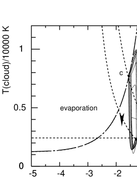
Figure 1: Evolution of the full system from the initial state (marked ‘a’) until the completion of the first few oscillations (solid line). The dashed lines descending to the right are the loci where the system switches from evaporation and condensation (lower curve, at point ‘b’) and vice versa (at point ‘c’). The horizontal dashed line is the locus of the evaporation funnel and the dot-dashed curve depicts the condensation funnel (see text).

In Fig. 1 we show the track in the ($g-T_{c}$)-plane of a model entering the oscillatory mode and performing a few cycles. Starting from a point marked ‘a’, it quickly and rather directly enters a limit cycle. At point ‘b’ the system changes over from evaporation to condensation. While just a little amount of gas is condensed, the clouds heat up rapidly to a maximum, then cool along the dot-dashed curve, while much more gas condenses. This continues to point ‘c’ where the system changes over to evaporation. Cooling in the clouds follows, with initially little gas return which increases thereafter. Passing through a minimum temperature, the clouds reach a temperature marked by the horizontal dashed line, along which the system reaches again point ‘b’ and switches back to condensation. As will be shown below, the horizontal dashed line is identified as the self-regulated star-formation mode; the passage through the temperature minimum is merely the transient while the system settles into equilibrium (Köppen et al. 1995).

The two dashed curves sloping down to the right delineate the border where the system changes between evaporation and condensation. One notices that points ‘b’ and ‘c’ do not lie on the same curve. This is because the gas temperature $T_{g}$ at point ‘b’ is about 10 percent lower than at point ‘c’. Though this amplitude is rather modest, the strong dependence of the switch criterion on $T_{g}$ leads to a strong shift of the switch curve in the diagram. But these oscillations in $T_{g}$ are not essential for the behaviour of the model.

3.2 Origin of the oscillations

The fact that the numerical simulations show the appearance of the oscillations primarily in cloud temperature and gas density indicates that these two variables form an ‘inner’ system whose behaviour is governed by the values of the control parameters $(c,T_{g})$. A most convenient way to analyze this is plotting the streamlines of the equations in the ($g-T_{c}$)-plane, with the other variables $c$, $s$, and $T_{g}$ either changing with time or held constant. We find that for the explanation of the fundamental structures, the exact dependences of the rate coefficients on density or temperature as given by McKee & Begelman (1990) or Cowie et al. (1981) are of secondary importance. It is completely sufficient to assume that the rate coefficients for condensation and evaporation are constant ($K,E$). In the following, we regard this simplified description; for the criterion of switching between condensation and evaporation, the prescription to compute $\sigma$ is kept as given above, but we shall consider the threshold value of 0.03 as another free constant $\sigma_{0}$.

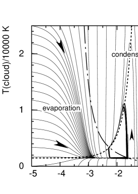
Figure 2: The overall behaviour of the simplified system: streamlines for the combined equations. The dot-dashed curve is the locus where the clouds change from condensation to evaporation, the short dashed lines mark the funnels. All streamlines below the horizontal dashed line point upwards.

The resulting streamlines are shown in Fig. 2, which corresponds to Fig. 1 except for the slightly different position of the limit cycle. One distinguishes the two different regions of evaporation and condensation. In the evaporation regime, all streamlines are always oriented towards increasing gas density, and bunch together to form a funnel centered at constant $T_{c}\approx 1800$ K (corresponding to $T_{c}=2400$ K in Fig. 1). Along this feature, the clouds evaporate at constant temperature, until the gas density exceeds a critical value – corresponding to point ‘b’ in the full model – and condensation commences. Setting $K=0$ in Eqns. 1, 2, and 18 and using $\raisebox{1.07639pt}{$\stackrel{{\scriptstyle.}}{{e}}_{c}$}=b(\raisebox{1.07639pt}{$\stackrel{{\scriptstyle.}}{{c}}$}T_{c}+c\raisebox{1.07639pt}{$\stackrel{{\scriptstyle.}}{{T}}_{c}$})$, one gets the equation for the streamlines:

$${dT_{c}\over d\ln g} = g{\raisebox{1.07639pt}{$\stackrel{{\scriptstyle.}}{{T}}_{c}$}\over\raisebox{1.07639pt}{$\stackrel{{\scriptstyle.}}{{g}}$}}=g{h_{c}s-c^{2}\Lambda(T_{c})\over bc(s\eta/\tau+Ec)}$$

At $g=0$ all streamlines are horizontal, which is merely a feature of the logarithmic representation and gives the impression of the fan structure on the left as the lines bunch together into the funnel. The important horizontal streamline along the funnel is described by the balance between stellar heating and radiative cooling $h_{c}s=c^{2}\Lambda$, i.e. the evolution proceeds with the clouds being essentially in thermal equilibrium. As these are the only features, it is evident that regardless of its initial state, the system will always end up in the funnel, along which it evolves at constant cloud temperature towards higher gas densities.

Figure 3: Similar to Fig. 2, but showing the case for pure condensation, and assuming a temperature of the condensate $\tilde{T}_{g}=20\,000$ K. On the dashed line thermal equilibrium in the clouds exists, the dot-dashed line shows where the cloud temperature is constant.

In the condensation regime, all streamlines are oriented towards lower gas densities. Here, one finds a funnel, marked by the short-dashed curve sloping down from upper right to lower left. All streamlines, whether coming from lower or higher temperatures, merge into this funnel which meets the switch line at $\lg(g)=-2.3$ and $T_{c}\approx 3000$ K, and the system is changed back to evaporation corresponding to point ‘c’ in Fig. 1. Setting $E=0$ yields the equation for the streamlines

$${dT_{c}\over d\ln g} = g{(h_{c}s-c^{2}\Lambda(T_{c}))+bKg(\tilde{T}_{g}-T_{c})\over bc(s\eta/\tau-Kg)}$$

Figure 3 depicts the whole condensation regime in the ($g-T_{c}$)-plane. To show the behaviour at large densities, a lower value of $\tilde{T}_{g}=20\,000$ K is assumed. Apart from a region of horizontal streamlines at $g=0$, as for the evaporation region, one finds these structures:

• at low gas densities, a horizontal streamline exists where $h_{c}s=c^{2}\Lambda$, the same condition as for the evaporation funnel. Its position agrees closely with the upper short dashed curve in Fig. 3, which is the locus where one has thermal balance in the clouds $\raisebox{1.07639pt}{$\stackrel{{\scriptstyle.}}{{e}}_{c}$}=0$.

• at large gas densities, a horizontal streamline appears where $T_{c}=\tilde{T}_{g}$. The dot-dashed curve (labeled ‘A’) shows where the cloud temperature does not change with time. The clouds are not in thermal equilibrium, because the condensation occurs faster than the cooling time, and the clouds are kept at the condensates’ temperature.

• both two parts are connected with a curve, along which the evolution proceeds towards thermal equilibrium in the clouds. Where the transition occurs, is essentially determined by the ratio of $\Lambda$ and $b(gK/c^{2})(\tilde{T}_{g}-T_{c})$.

• there is an additional feature, showing up as a clump of streamlines: the intersection of the condensation funnel with the condition $s\eta/\tau-Kg=\raisebox{1.07639pt}{$\stackrel{{\scriptstyle.}}{{g}}$}=0$ at $\lg g=-2.6$ and $T_{c}=1800$ K (in Fig. 3) forms an attracting node. The evolution of the clouds proceeds in thermal equilibrium and in balance between stellar gas return and condensation.

Independent of the initial conditions, the system always reaches the condensation funnel, where the clouds cool and the gas density decreases. However, under certain conditions, the system may enter an equilibrium evolution at constant gas density.

The overall evolution can thus be pieced together: The two regimes of evaporation and condensation are separated by the curve where the criterion of Cowie et al. (1981) is met exactly ($\sigma=\sigma_{0}=0.03$), depicted in Fig. 2. One may work out how the position of this switching line depends on the parameters, using the prescriptions (Eqns. 6 to 2.1). For a cloud filling factor much smaller than unity, which is the common case, one obtains:

$$\sigma=4.18\cdot 10^{-17}\cdot T_{g}^{2.5}\,T_{c}^{-1}\,g^{-0.5}$$ (23)

The curve’s location is independent of the cloud density $c$, and it is shifted towards lower gas densities, if one raises the threshold $\sigma_{0}$ or lowers the gas temperature $T_{g}$, which is the most sensitive parameter.

The existence of the funnels makes it relatively easy to predict the conditions under which oscillations occur. From the pattern of the streamlines it is clear that a condition for a closed track in the plane is the intersection of evaporation funnel and switching line should happen at a lower cloud temperature (and higher gas density) than that of condensation funnel and switch curve. The conditions for the funnels and the switch line constitute a set of simultaneous non-linear equations which can be solved numerically to yield the curve in the $(g-T_{c})$-plane, and the positions of the intersections. The stellar density can be estimated from the low density limit $s\approx\xi\tau\Psi$ (cf. Köppen et al. 1995). The geometry of the funnels thus allows a classification of the behaviour, as a function of the ‘outer’ parameters $c$ and $T_{g}$, as shown in Fig. 4. Furthermore, the difference and ratio of the densities $g$ can be used together with the two forms of Eqn. 1 to estimate the times spent in each phase, the oscillation period and the keying ratio. Because these considerations neglect the changing gas temperature, they predict the types of behaviour of the complete network only in a qualitative way.

Figure 4: The behaviour of the simplified system as a function of the control parameters $c$ and $T_{g}$, as estimated with the assumption of constant stellar density: Circles denote where oscillations occur (filled circles: the gas temperature is within a factor of 2 of the value for thermal equilibrium of the gas). In the white area, oscillations also occur, but with a period of over 5 Gyrs. Plus-signs indicate where the streamlines in both regimes are too flat, and the system comes to rest at an intermediate point on the switching line. Small dots show when the funnels meet very closely, and the asterisks indicate that the system enters the $\raisebox{1.07639pt}{$\stackrel{{\scriptstyle.}}{{g}}$}=0$ equilibrium.

All these investigations – together with numerical solutions of the complete system – show that oscillations are restricted to a finite range in cloud density, which may be quite narrow (less than a decade) and which is rather sensitive to some of the parameters and constants in the model.

During a cycle, the following sequence of physical processes takes place: When condensation starts, the clouds are rapidly heated up by the gas condensates, until the condensation funnel is reached. There, the clouds cool radiatively and evolve towards thermal equilibrium. When the switching criterion is met again, evaporation commences. Lacking the heating by the condensates, the clouds cool until the new thermal equilibrium is reached. Then the on-going evaporation of the clouds increases the gas density, until the condensation criterion is again fulfilled.

The cycle is thus essentially driven by the deposition of thermal energy of the condensates into the clouds, which radiate the energy away in the form of line emission. Thus the source which makes the cycle possible is the deposition of sufficiently hot material onto the clouds. The temperature $\tilde{T}_{g}$ of the condensates is an extremely sensitive parameter: oscillations can only be found if the condensing gas remains hot $\tilde{T}_{g}=T_{g}$. Assumption of a lower temperature greatly reduces the region for the occurrence of oscillations, or can completely suppress them. This is quite easily understood in terms of the condensation funnel (Fig. 3): the position of its high-density branch is determined by the condensate temperature. Any cooling reduces the range in cloud temperatures that the funnel covers and thus the possibility for having a cyclic path between the two regimes is reduced. Thus, the prescription of the transfer of energy during the condensation phase is a most critical part of the network.

4 The physically consistent formulation

McKee & Cowie (1977) and McKee & Begelman (1990) give expressions for the mass transfer rate, but not for the rate of energy exchange between gas and clouds. Therefore one considered in the previous chemodynamical models (e.g. Theis et al. 1992) limiting cases, such as that the condensing gas does not cool or cools down to some fixed temperature. Forming only one of the many processes of the ISM model network, this rather simple recipe was preferred. Of course, it is not a physically entirely satisfactory description, even more so since the oscillations were found to be rather sensitive to the exact recipe.

A physically consistent prescription can be formulated from noting that McKee & Cowie (1977) as well as McKee & Begelman (1990) derive their evaporation and condensation rates on the basis of a stationary solution for the gas flow between cloud and intercloud matter, with a fixed temperature profile. This means that any parcel of condensing gas follows the local temperature from the intercloud gas to the cloud interior, and that it arrives in the cloud with the cloud’s temperature: $\tilde{T}_{g}=T_{c}$. As discussed above, cooling of the condensating material results in a lowering of the high-density part of the condensation funnel (cf. Figs. 2 and 3). If now the condensates cool down to the cloud temperature, the condensation funnel is merely a horizontal line, at the same height of the evaporation funnel. Because of the opposite directions of the streamlines in the two regimes, the intersection of the funnels – which are characterized by thermal balance in the clouds – with the switching curve is an attracting node, in which the system will always end up. Here, the system evolves with the cloud gas in thermal equilibrium, and without any oscillations.

The switching condition implies that $Ec=Kg$ (Eqn. 15) and so the evaporation and condensation terms in Eqns. 1, 2, 16, and 18 vanish. Usually one finds that $g\ll c$, so that one has $c\approx c+g$, and the overall evolution is described by

$${d\over dt}(c+g) = -\Psi+s\eta/\tau$$

$$\stackrel{{\scriptstyle.}}{{s}} = \xi\Psi-s/\tau$$

$$\stackrel{{\scriptstyle.}}{{r}} = (1-\xi)\Psi+(1-\eta)s/\tau$$

$$\stackrel{{\scriptstyle.}}{{e}}_{c} = h_{c}s-c^{2}\Lambda(T_{c})-\Psi bT_{c}$$

which is nothing but the single-gas-phase system which has been shown to evolve almost exclusively in an equilibrium between star-formation and its inhibition due to the heating of the ambient gas by the massive stars (Köppen et al. 1995).

Note that in this more general view, the conversion of gaseous matter into remnants is independent of the rate coefficients for evaporation and condensation, and even on the actual prescription for the switching. But how the gas is divided among clouds and intercloud gas, depends on these specifications.

The switching of the system between condensation and evaporation gives rise to non-continuous terms in the differential equations. However, since in both regimes the system evolves towards the switching condition, this apparent mathematical difficulty makes the solution instead more simple: It forces the system to evolve along the switch line.

This permits to estimate the timescales of the equations: For conditions appropriate to a galactic disk ($c=0.1$ M_⊙/pc³) one has $T_{c}\approx 3000$ K from the figures shown. The gas density is typically $g\approx 0.1...0.01c$. The cloud filling factor is usually quite small $\epsilon_{c}=cT_{c}/gT_{g}\ll 1$. From Eqn. 23, one gets for the temperature of the intercloud gas

$$T_{g}=8.76\cdot 10^{5}\,{\rm K}\,\cdot(\sigma_{0}/0.03)^{0.4}\,\cdot T_{c}^{0.4}\,g^{0.2}\approx 10^{7}\,{\rm K}$$ (24)

which is quite insensitive to the actual gas density. The rate coefficients are obtained from Eqns. 6 to 14

$$E = 1.17\cdot 10^{-17}\cdot T_{g}^{2.5}\,T_{c}^{-1}\approx 0.001\,{\rm Myr}^{-1}$$

$$K = E\cdot{c\over g}\approx 0.01...0.1\,{\rm Myr}^{-1}.$$

This makes these processes much slower than the cooling in the clouds $\tau_{\rm cool,c}=bT_{c}/c\Lambda\approx 0.4$ Myr, but faster than star-formation $\tau_{\rm SFR}=c/\Psi\approx 300$ Myr. For larger heating coefficients than we used here, the star-formation is even slower (few Gyr), and the two equilibria influence each other even less.

Thus, after some transient phase, the evolution proceeds in a hierarchy of equilibria: the fast cooling in the clouds will establish the self-regulated mode of star-formation; on a longer timescale the condensation and evaporation will balance the distribution of the gaseous matter among cloud and intercloud gas; and even more slowly, all gas is consumed to be turned into stellar remnants.

4.1 Balance of condensation and evaporation

How the gas is distributed among the gas and the cloud component, depends on the condensation and evaporation. As stated above, the system evolves along the switching line, which can be formulated as:

$$0={d\ln(\sigma)\over dt}=2.5\,{\raisebox{1.07639pt}{$\stackrel{{\scriptstyle.}}{{T}}_{g}$}\over T_{g}}-0.5\,{\raisebox{1.07639pt}{$\stackrel{{\scriptstyle.}}{{g}}$}\over g}-{\raisebox{1.07639pt}{$\stackrel{{\scriptstyle.}}{{T}}_{c}$}\over T_{c}}$$

Thermal equilibrium in the clouds implies constant temperature, so the last term vanishes, and with Eqn. 16 one gets

$${\raisebox{1.07639pt}{$\stackrel{{\scriptstyle.}}{{g}}$}\over g}=5\,{\raisebox{1.07639pt}{$\stackrel{{\scriptstyle.}}{{T}}_{g}$}\over T_{g}}=5\,{h_{g}s-g^{2}\Lambda(T_{g})\over bgT_{g}}$$

The changes of the densities can be written in the low density limit of self-regulated star-formation $s\approx\xi\tau\Psi\approx 0.03\,c^{2}$

$$\stackrel{{\scriptstyle.}}{{g}} = a_{1}\,\,g^{-0.2}(\sigma_{0}/0.03)^{-0.4}[a_{2}\,\,c^{2}-a_{3}\,\,g^{2.1}(\sigma_{0}/0.03)^{0.2}]$$

$$\stackrel{{\scriptstyle.}}{{c}} = -(1-\xi\eta)\Psi-\raisebox{1.07639pt}{$\stackrel{{\scriptstyle.}}{{g}}$}$$

where $T_{g}$ is taken from Eqn. 24, and using the abbreviations

$$a_{1} = 1.79\,10^{-5}\cdot(T_{c}/3000\,{\rm K})^{-0.4}$$

$$a_{2} = 0.03\cdot h_{g}\approx 660$$

$$a_{3} = 8.36\,10^{4}\cdot(T_{c}/3000\,{\rm K})^{0.2}$$

One notes that the equations have a critical point which obeys the condition $a_{2}c^{2}=a_{3}g^{2.1}(\sigma_{0}/0.03)^{0.2}$, or

$${g\over c}\propto c^{-1/21}\,\,\sigma_{0}^{-2/21}$$

Thus the ratio $g/c$ due to the balance of condensation and evaporation increases only very slightly as the cloud gas is consumed. It is independent of the actual rate coefficients, and only weakly dependent on the switching threshold. These properties are found in the numerical solutions, shown in Fig. 5. After the transient evolution subsides – within 1 Gyr, which depends on the rate coefficients – the system enters the equilibrium, where the above derived dependences are obeyed. This shows that, apart from transient phases, the results of the chemo-dynamical models are quite insensitive to the details of the recipe of Cowie et al. (1981), for example the correction factor $\Phi$ for the influence of magnetic fields.

Figure 5: The mass ratio of gas and clouds, as a function of cloud density, for different values of the switching threshold $\sigma_{0}$.

The stability of the system against perturbations of the gas and cloud densities and temperatures are investigated by numerical experiments, adding or removing a substantial (50 percent) portion of the gas present in the system or changing strongly the temperatures. After a transitory phase lasting some 100 Myrs, a new equilibrium solution is reached which has the same character as before, i.e. without oscillations. In the transient there may be a few bumps and wiggles, but the system never breaks into oscillations. This is as expected, since the disturbance moves the system in e.g. the $(g-T_{c})$-plane to another position, from where it always evolves towards one of the funnels to end up in the intersection with the switch line. Since the character of the streamlines cannot be altered into the pattern responsible for oscillations, the system is also very robust against inflows, outflows, and external heating.

4.2 Metallicity

In Fig. 6 we depict the relation of abundance in the cloud component of a primary element with the gas fraction $f_{\rm gas}=(c+g)/(c+g+s+r)$. In the Simple Model (closed-box with instantaneous recycling) the gas metallicity follows $Z=-y\ln{f_{\rm gas}}$ with the true yield $y$, shown as the dashed line. For simplicity, we divide the abundances by the yield. The abundance rises more steeply at early times than the Simple Model, because we allow for a finite life-time of the massive stars which are responsible for the metal enrichment.

For comparison, we also show the model where the condensing gas does not cool: the metallicity remains constant during the evaporative phases, separated by a steep rise when the metal-rich gas is mixed to the clouds at the beginning of the condensation phase. If one allows the gas to cool down to cloud temperature before condensing, after a single evaporative intervall, the evolution proceeds in what seems to be the average evolution of the model with oscillations. It is worth emphasizing that for $\lg(-\ln(f_{\rm gas}))>-0.2$, the evolution of either model is quite close (within 0.1 dex) to that of the Simple Model, i.e. the effective yield is nearly equal to the true yield.

In Fig. 7 we show the behaviour of the abundance of a secondary element such as nitrogen, by the N/O vs. O/H plot. The Simple Model predicts a strictly linear relationship, viz. a straight line with slope 1 for the logarithmic values. Apart from a systematically lower yield for nitrogen (by 0.1 dex), the numerical models show a quite similar slope. The oscillations are less noticeable here than in the abundances themselves, and in the overall evolution, they make the slope of the N/O-O/H relation steeper. If one allows for cooling of the condensing gas, the slope is very close to unity.

Thus, in both aspects, the chemical enrichment of the clouds from which the stars are born occurs in the very much same way as in the Simple Model. This should not be too surprising, because we do consider a closed-box model. Moreover, the time-scales for mixing of the freshly-produced metals into the cloud gas are determined by the condensation/evaporation times, which are still short compared to the overall evolution, viz. the gas consumption.

Figure 6: The abundance of a primary element (oxygen) in the clouds as a function of the gas fraction $f_{\rm gas}=(c+g)/(c+g+s+r)$. Shown are models with constant evaporation/condensation rate coefficients, assuming that the condensates retain the gas temperature (stepped curve) or cool down to the cloud temperature. The behaviour of the Simple Model is shown as a dashed line.

Figure 7: The evolution of the abundances of a secondary (nitrogen) and a primary element (oxygen), for the same models shown in Fig. 6.

5 Models with simultaneous evaporation and condensation

The models that treat the clouds as being identical are certainly a simplification. For a more realistic approach, one would consider a cloud population with a distribution in e.g. mass, as is done in the models of Samland et al. (1997). With such a description of the cloud phase, the Cowie et al. criterion implies that all clouds smaller than a certain radius will evaporate, while those larger will grow by condensation. Thus, one has at the same time both processes taking place, and for the overall rates one integrates over the cloud spectrum. How this is done and which rates one gets, depends on any further assumptions on the evolution of the cloud population. Samland et al. obtain for the solar neighbourhood, coefficients $E\approx 10^{-3}$ Myr^-1 and $K\approx 0.1$ Myr^-1 which remain quite constant throughout the evolution.

Such a system settles quickly, within a few condensation time-scales $\tau_{\rm cond}$ into the balance between condensation and evaporation

$${g\over c}={E\over K}$$

which is time-independent. The overall gas consumption takes place much more slowly, with $\tau_{\rm SFR}$. For a linear SFR, this can easily be shown by solving the equations analytically. Since one normally has $\tau_{\rm SFR}>\tau_{\rm evap}>\tau_{\rm cond}$, most of the gaseous matter is in the cloud component, which is slowly converted into stellar remnants.

In Fig. 8 we show the ratio $g/c$ as a function of cloud density for models with $E/K=0.1$, starting with an initial density $c=10^{0.5}\,\,{\rm M}_{\odot}/{\rm pc}^{3}$. The self-regulated star-formation is quickly established as soon as the star-formation time-scale has become larger than the mean life-time of the massive stars ($c/\Psi>2\tau$ or $c<10^{0.2}$). As long as the condensation occurs faster than the stellar gas return ($K>0.1$ Myr^-1), the system settles into the condensation/evaporation equilibrium. In models with very low condensation coefficients, the ejecta from the stars formed in the initial period of rather high star-formation are first accumulated in the hot gas, whose mass may remain constant while the clouds continue to be consumed – $g/c\propto 1/c$. After a few condensation time-scales the gas condenses following the steady-state condition (Eqn. 5). The peak in the curve for the rather extreme model with $K=0.001$ at $\lg c=-1$ marks where the gas and cloud phases are in equilibrium. In this model, about 10 percent of the initial mass is present in the gas component for about a few Gyr.

Figure 8: The mass ratio of gas and clouds, as a function of cloud density, for different values of the condensation rate coefficient $K$ (in Myr^-1), and with the same ratio $E/K=0.1$.

In Fig. 9 we show the ratio of the metallicities in gas and cloud components, to study the efficiency of the mixing between the two components. Comparing with the evolution of the density ratio, one notices that the metallicities become equal as soon as the model reaches the steady-state solution (Eqn. 5).

Figure 9: Like Fig. 8, but for the ratio of the oxygen metallicities. The dashed line is a model with $K=1$ and $E=0.01$.

The oxygen abundance in gas and clouds as a function of the gas fraction is depicted in Fig. 10, compared to the expectation from the Simple Model. If condensation and evaporation occur faster than star-formation, gas and clouds remain well-mixed, and the model follows the Simple Model very closely. The metallicity of the clouds is essentially determined by the amount of mixing due to condensation, it does not depend on the value of $E$. On the other hand, the gas metallicity is determined by how much the stellar ejecta are mixed with the low metal material evaporated from the clouds. For low values of $E$ the mixing is poor, and the metallicity is as large as the metal abundance of the fresh stellar ejecta which is as large as $y/\xi\approx 10y$ (Eqn. 19). Eventually, all models evolve with the true yield.

In systems with a large initial density $c_{0}\geq 1$ M_⊙/pc³ (shown in Fig. 11) the initial SFR $\Psi\approx 0.03c^{2}_{0}$ is greater than the condensation rate $gK\approx(0.1...0.01\cdot c_{0})\cdot 0.1$. As a consequence, metals accumulate in the gas, and because of the small but existing reprocessing of enriched cloud matter the metallicity even rises. The condensation of the metal-rich gas occurs only at a more evolved stage, and then the large gas metallicity causes the clouds to have metallicities larger than expected from the Simple Model.

Figure 10: The oxygen metallicity as a function of the gas mass fraction, for the intercloud gas (and for different values of the evaporation rate coefficient $E$) and the clouds (independent of $E$). The condensation coefficient is $K=0.1$, the initial cloud density is $c_{0}=0.1$ M_⊙/pc³. The behaviour of the Simple Model with a unity yield is shown as a dashed line, the short dashed lines for half and double yield.

Figure 11: Same as Fig. 10, but with a higher initial cloud density $c_{0}=10$ M_⊙/pc³.

5.1 Distribution of metal mass among the components

In a galaxy, the total mass of a primary element such as oxygen is proportional to the total number of type II supernovae that have exploded until the present time, independent of when and where this happened. This makes the total metal mass an essential indicator for the global state of a galaxy, though it is not easy to obtain, as it requires the determination of not only the mean abundances of gas in the various forms and stars, but their mass fractions as well. This would involve different wavelength regions and abundance analysis techniques with the problems associated combining the data.

Is it necessary to measure all gaseous components, or would the observation of a single phase, e.g. the cloud components being observable with H II regions, suffice? What is the magnitude of the errors involved? In the following, we use our closed-box chemodynamical models to provide some rough answers. Since the freshly produced metals are first injected into the warm or hot intercloud gas, observations of the dense cloud medium might miss an important fraction of the metals.

In Figs. 12 to 14 we show how the distribution of oxygen mass over gas, clouds, and remnants depends on the gas mass fraction $f_{\rm gas}$, which indicates the chemical age of a system. The metals in chemically very young systems are still mainly in the hot gas. At more advanced stages, the metal rich gas has condensed into the clouds, which then contain most metal mass. In highly evolved systems, the metals are found in the remnants. The shape of the curves in intermediately evolved systems, i.e. around the peak of the contribution from the clouds, is mainly determined by the ratio of the inverse time-scales for condensation and initial star formation $K/(\Psi/c_{0})\propto K\cdot c_{0}$. Because in the closed-box model most of the star formation occurs during the initial phase, this time-scale determines how much metals are produced and which are released from the intercloud medium by condensation $K$. For $K\cdot c_{0}<1$ M_⊙pc^-3 Myr^-1 (Fig. 12) the metals are hardly to be found in the gas, because of the rapid condensation into clouds. For values smaller than about 0.1 (Fig. 14) the metals remain in the gas until rather late, and because of the fast conversion of clouds into stars, they are swiftly locked up into remnants. As the clouds may contain less than a third of all the metals, measurements of the metallicity of the cloud gas only could be rather misleading for the determination of the total metal mass in a galaxy. Such a situation arises for low condensation rates or for high initial gas densities, i.e. a centrally rather concentrated proto-galactic cloud.

The shapes of the curves are much less strongly influenced by the ratio $E/K$ which we kept constant in the figures: It determines the ratio of metal mass contained in gas and clouds in the late evolution; thus because one has $E<K$, the clouds keep a larger portion of the metal mass than the gas.

Figure 12: The fraction of the oxygen mass in the gas, clouds, and remnants, as a function of the gas mass fraction $f_{\rm gas}$. Model parameters are $c_{0}=0.1$ M_⊙/pc³, $K=0.1$ Myr^-1, and $E/K=0.01$.

Figure 13: Same as Fig.12 but with $K=0.01$ Myr^-1.

Figure 14: Same as Fig.13 but with an initial density $c_{0}=10$ M_⊙/pc³.

6 Conclusions

We investigate the behaviour of one-zone chemical evolution models which utilize the chemodynamical prescription for a two-component interstellar medium. This is done by numerical solution, topological analysis of the equations, and identification of the conditions for equilibrium solutions.

The self-regulated star-formation found in models with a single gas component (Köppen et al. 1995) is not at all disturbed by the additional condensation and evaporation processes. Due to its shorter time-scale, it dominates the evolution. The models follow the self-regulated solution very closely, without any oscillations.

On the other hand, it is the distribution of the gas among the cloud and intercloud phases which is determined by the mass exchange due to condensation and evaporation. The evolution also follows an equilibrium which is either ruled by the switching condition $\sigma=\sigma_{0}$ or by the relation $gK=Ec$. The mass of gas in the intercloud phase is usually very small compared to that found in clouds.

From realistic rate coefficients for condensation and evaporation in a cloud population (Samland et al. 1997) one finds that the evolution of the model follows a hierarchy of nested equilibria, which are in ascending order of their quite separate time-scales: thermal equilibrium in the cloud gas, regulation of the SFR by heating of gas due to radiation from massive stars, equilibrium of mass exchange between gas and clouds. This is further embedded into the overall conversion of gas into stellar remnants.

During the evolution in the equilibrium between condensation and evaporation $gK=Ec$, the relation between metallicity and gas mass fraction follows a Simple Model quite closely. Gas and cloud phases are well-mixed, their metallicities are the same.

Together with the quadratic dependence of the star-formation rate on the cloud density (cf. Köppen et al. 1995), these aspects make up the global behaviour that is typical for chemo-dynamical evolution models.

In models with low condensation coefficients and/or high initial cloud densities, the metal-rich gas ejected by the stars formed in the initial period of intense star-formation may remain in the intercloud medium quite long, before condensation into clouds commences and metal enrichment of the clouds occurs.

From these models we compute how the total metal mass in a galaxy is distributed among gas, clouds, and stellar remnants and how this changes with the chemical age of the system. For conditions similar to the solar neighbourhood, unevolved gas-rich systems have their metals in both cloud and intercloud gas. In high-density models (or those with small condensation rates) the metals may remain in the intercloud medium even in rather evolved, gas-rich galaxies, and those contained in the cloud phase may be a rather portion. Work is under way to investigate the properties of full ‘chemodynamical’ models with the complete network of interactions and the coupling to the global dynamics.

Acknowledgements: We thank M. Samland and R. Spurzem for valuable discussions. J.K. thanks the Deutsche Forschungsgemeinschaft for financial support (project He 1487/13-1) and the Observatoire de Strasbourg for its generous hospitality.

References

- [1] Cowie L.L., McKee C.F., Ostriker J.P., 1981, ApJ 247, 908
- [2] Götz M., Köppen J., 1992, A&A 262, 455
- [3] Habe A., Ikeuchi S., Tanaka Y.D., 1981, PASJ 33, 23
- [4] Hensler G., Burkert A., 1991, in: Proc. Elba Workshop ”Chemical and Dynamical Evolution of Galaxies” eds. F.Matteucci et al., p.168
- [5] Ikeuchi S., Habe A., Tanaka Y.D., 1984, MNRAS 207, 909
- [6] Köppen J., Arimoto N., 1991, A&AS 87, 109 and 89, 420
- [7] Köppen J., Theis Ch., Hensler G., 1995, A&A 296, 99
- [8] McKee C.F., Begelman M.C., 1990, ApJ 358, 392
- [9] McKee C.F., Cowie L.L., 1977, ApJ 215, 213
- [10] McKee C.F., Ostriker J.P., 1977 ApJ 218, 148
- [11] Pagel B.E.J., Patchett B.E., 1975, MNRAS 172, 86
- [12] Samland M., Hensler G., Theis Ch., 1997, ApJ 476, 544
- [13] Theis Ch., Burkert A., Hensler G., 1992, A&A 265, 465