Helmet Streamers with Triple Structures:
Weakly Two-Dimensional Stationary States

Abstract

Recent observations of the solar corona with the LASCO coronagraph on board of the SOHO spacecraft have revealed the occurrence of triple helmet streamers even during solar minimum, which occasionally go unstable and give rise to particularly huge coronal mass ejections. We present a method to calculate (semi-)analytically self-consistent stationary configurations of triple helmet streamers which can serve as input for stability considerations and dynamical calculations. The method is based on an asymptotic expansion procedure using the elongated structure of the streamers. The method is very flexible and can be used in both Cartesian and spherical geometry. We discuss the effects of magnetic shear, gravity and field-aligned flow on open field lines. Example solutions illustrating the influence of each of these features on the solution structure are presented.

1 Introduction

Recent observations of the corona with the LASCO coronagraph [Schwenn et al. (1997)] on board of the SOHO spacecraft showed that the corona can be highly structured even during the solar activity minimum. The observations revealed a triple structure of the streamer belt which was existent for several consecutive days. The observations further showed that these triple structures occasionally go unstable leading to a seemingly new and extraordinarily huge kind of coronal mass ejection (global CMEs). Natural questions arising from these observations are whether the helmet streamer triple structure is directly connected with or responsible for the occurrence of global CMEs and what is the physical mechanism of their formation. The aim of this paper is to provide a first step towards a better theoretical understanding of these phenomena.

The structure of helmet streamers and their stability has been studied both observationally and theoretically for a long time (e.g. Pneuman and Kopp, 1971; Cuperman et al., 1990; Cuperman et al., 1992; Koutchmy and Livshits, 1992; Wang et al., 1993; Cuperman et al., 1995; Wu et al., 1995; Hundhausen, 1995; Bavassano et al., 1997). A natural association seems to exist between helmet streamer stability and coronal mass ejections (CMEs) and sometimes CMEs are accompanied by erupting prominences or filaments. Coronal streamers are also thought to be the source regions of the slow solar wind and the activity processes discussed above may well contribute to this component of the solar wind.

Multiple streamer structures have already been observed before SOHO, however mainly during the maximum phase of the solar activity cycle. Also, observations of the heliospheric plasma sheet seem to indicate a multiple current sheet substructure of the plasma sheet itself Crooker et al. (1993); Woo et al. (1995) which has initiated several theoretical investigations of the stability of multiple current sheets Otto and Birk (1992); Yan et al. (1994); Dahlburg and Karpen (1995); Birk and Otto (1997); Birk et al. (1997); Wang et al. (1997).

The aim of this work is to present a simple method by which triple helmet streamer structures can be calculated self-consistently. We want to keep the method simple enough so that we can obtain largely analytical results without rendering our models too unrealistic. Since the observed structures seem to be quite elongated (the radial magnetic field component is considerably larger than the longitudinal magnetic field component), we can employ a method which has already been applied very successfully to the equilibrium structure of the magnetotail of the Earth Schindler (1972); Birn et al. (1975). The method is based on an asymptotic expansion. Here we generalize this method and show how it can be applied to find solutions with internal multiple structures. Obvious generalizations of the original magnetospheric versions to solar applications are the use of a more suitable coordinate system (spherical rather than Cartesian), the inclusion of magnetic shear, of the solar gravity field for large scale structures and of plasma flow on open field lines. For reasons of mathematical simplicity and since we only deal with the subcritical part of the flow, we confine the discussion to incompressible flow. Our models provide a flexible quantitative description of structured helmet streamers. They can also be used as the starting configurations for future studies of the dynamical evolution of such structures.

The outline of the paper is as follows. In Sect. 2 we present the mathematical basis of the method. Section 3 contains representative results obtained by applying the method under various sets of assumptions. In Sect. 4 we summarize the paper, give a discussion of our results and an outlook on future work.

2 Mathematical Formulation

2.1 Basic equations

We use the equations of stationary ideal magnetohydrodynamics to describe the coronal plasma:

$$-\nabla P+\frac{1}{\mu_{0}}(\nabla\times{\bf B})\times{\bf B}-\rho\nabla\Psi = \rho{\bf v}\cdot\nabla{\bf v}$$ (1)

$$\nabla\cdot(\rho{\bf v}) = 0$$ (2)

$${\bf E}+{\bf v}\times{\bf B} = 0$$ (3)

$$\nabla\cdot{\bf B} = 0$$ (4)

$$P = \rho RT.$$ (5)

Here, $P$ stands for the plasma pressure, $\bf B$ for the magnetic field, $\rho$ for the plasma density, $\Psi$ for the solar gravitational potential, $\bf v$ for the plasma velocity, $\bf E$ for the electric field, $R$ is the gas constant, $T$ the temperature and $\mu_{0}$ the vacuum permeability. Due to the high conductivity of the coronal plasma the magnetic field is frozen into it (Eq. 3) and we can make the assumption that the observed plasma features outline the magnetic field structure. Throughout the rest of the paper we make the following assumptions:

• The streamer structure is very extended in azimuth and varies only very slowly along this direction (this assumption is supported by the observations Schwenn et al. (1997) which showed that the triple structure existed for several days); we can then describe the structure as approximately two-dimensional in the sense of rotational invariance.

• The streamers are elongated in the radial direction and the radial magnetic field component is considerably stronger than the latitudinal component; this is the basic assumption allowing to apply an asymptotic expansion procedure.

• If flow is included, it is purely field-aligned and confined to the open field line region; since we describe only the low lying parts of the streamer structure the flow velocities should be subcritical and we will therefore only consider incompressible flow.

• For simplicity, we consider only isothermal equilibria; in principle, other temperature structures or even the inclusion of an energy equation into the scheme is possible.

In the following, we normalize the magnetic field by a typical value $B_{0}$, the plasma pressure $p$ by $B_{0}^{2}/\mu_{0}$ (where $p=1$ is the maximum value of $p$), the mass density $\rho$ by $B_{0}^{2}/\mu_{0}\mbox{R}T$, the length $L$ by a solar radius and the current density by $j_{y}=B_{0}/\mu_{0}\,L$.

2.2 Method

To demonstrate the method we first use a two-dimensional Cartesian geometry with no spatial variation in the $y$-direction ($\frac{\partial}{\partial y}=0$) and assume static structures (${\bf v}=0$) without magnetic shear ($B_{y}=0$). In other geometries the basic properties of the method stay similar though the details may vary due to the geometry.

Writing the magnetic field as

$${\bf B}(x,z)=\nabla A(x,z)\times{\bf e}_{y}$$ (6)

we find from equation (1) that the flux function $A$ has to obey the equation (e.g. Low 1975; Birn et al. 1978; Low 1980; Birn and Schindler 1981)

$$-\Delta A=\frac{\partial}{\partial A}\left(P(A,\Psi)\right)$$ (7)

With the assumption of a constant temperature and because $\Psi=\Psi(z)$ in Cartesian geometry we get:

$$P(A,\Psi)=P(A,z)=k(z)\,p(A)$$ (8)

with $k(z)=\exp(-(\Psi(z)-\Psi(0))/\mbox{R}T)$. For slow variation of $\Psi(z)$ with height $z$ one can neglect gravity and finds $k(z)=1$.

If we assume that the magnetic field perpendicular to the photosphere ($B_{z}$ in the Cartesian geometry) is much larger than the parallel component ($B_{x}$ in the Cartesian geometry), or in other words, that streamers are rather elongated in the radial direction, we can use the method of asymptotic expansion and apply it to Eq. (7). Mathematically stretched configurations are characterized by the ordering

$$\frac{\partial}{\partial x}=O(1)\Rightarrow B_{z}=O(1)\qquad\frac{\partial}{\partial z}=O(\epsilon)\ll 1\Rightarrow B_{x}=O(\epsilon)$$ (9)

If we neglect terms of the order $\epsilon^{2}$ in Eq. (7) we obtain after one integration with respect to $x$ :

$$\frac{\partial A}{\partial x}=\pm\sqrt{2\left(p_{0}-p(A)\right)}$$ (10)

where $p_{0}=p_{0}(z)$ is an integration constant (total pressure on the $z$-axis), which depends parametrically on $z$. We solve this differential equation by separation Birn et al. (1975):

$$x-x_{0}=\int_{A_{0}}^{A}\frac{dA}{\sqrt{2\left(p_{0}-p(A)\right)}}$$ (11)

and fix the constant $A_{0}=A(x_{0})$ so that $p(A_{0})=p_{0}$.

Unfortunately it is impossible to derive the pressure function $p(A)$ directly from the observations presently available. We will therefore choose $p(A)$ by a compromise between physical reasoning and mathematical simplicity. We do not choose pressure functions which have a too simple dependence on $A$ like $p(A)\propto\mbox{const.}$, $A$ or $A^{2}$ because solutions of this type are a) known to be linearly stable and b) have already been discussed in Wiegelmann Wiegelmann (1997). A popular and convenient choice is $p(A)\propto\exp(cA)$ because it corresponds to the physical assumption that the plasma is in local thermodynamic equilibrium and it has the mathematical advantage that one can find analytical solutions. Using

$$p(A)=k\exp(cA)$$ (12)

where $k$ may be a function of $z$ and $c$ may be positive or negative, we get from equation (11):

$$A(x,z)=-\frac{2}{c}\log\left\{\cosh\left[c\sqrt{\displaystyle\frac{p_{0}}{2}}(x-x_{0})\right]\right\}+\frac{1}{c}\log\left(\frac{p_{0}}{k}\right)$$ (13)

The components of the magnetic field are then given by

$$B_{z}=\frac{\partial A}{\partial x}=-\sqrt{2p_{0}}\tanh\left(c\sqrt{\frac{p_{0}}{2}}(x-x_{0})\right)$$ (14)

$$B_{x}=-\frac{\partial A}{\partial z}=-\frac{\partial A}{\partial p_{0}}\frac{\partial p_{0}}{\partial z}-\frac{\partial A}{\partial k}\frac{\partial k}{\partial z}$$ (15)

We remark that one cannot evaluate $\frac{\partial A}{\partial p_{0}}$ and $\frac{\partial A}{\partial k}$ in equation (15) directly because in general $x_{0}$ depends on $p_{0}(z)$ and $k(z)$ as well. The plasma pressure can be obtained from the Eq. (12)

$$p=\frac{p_{0}}{\cosh^{2}(\sqrt{\frac{p_{0}}{2}}c(x-x_{0}))}$$ (16)

and the current density $j_{y}$ from $j_{y}=\frac{\partial p}{\partial A}$:

$$j_{y}=cp=\frac{p_{0}c}{\cosh^{2}\left(\sqrt{\displaystyle\frac{p_{0}}{2}}c(x-x_{0})\right)}.$$ (17)

2.3 Triple structures

The method just outlined has been applied very successfully to calculate the structure of the Earth’s magnetotail Birn et al. (1975); Schindler und Birn (1982); Wiegelmann and Schindler (1995). However, since we want to apply this method to describe multiple streamer structures a few details of the method have to be changed though the basic approach stays the same.

In an arcade structure the direction of the $B_{z}$ component of the magnetic field changes its sign as one crosses the centre of the arcade. In a triple structure, one will therefore encounter three such changes as one moves across the structure. In a stretched configuration described by the asymptotic expansion procedure, the only possibility to achieve this is that the current density $j_{y}$ changes its sign between the streamers, or, in other words, in the central streamer the current flows in the opposite direction with respect to the two outer streamers. In terms of the sign of $B_{z}$ this means that in order to paste the three arcades continuously together, the $B_{z}$ component in the central streamer has to change just in the opposite sense to the outer two streamers.

Since the current density $j_{y}$ is directly linked to the plasma pressure by the relation $j_{y}=\partial P/\partial A$, this implies that the derivative of the pressure with respect to the flux function $A$ has to change its sign, too. We can therefore not use a single exponential function to model the pressure because the exponential function and its derivative have no zero. The simplest alternative is that we use different pressure functions for the middle ($p_{1}(A)$ say) and for the outer streamers ($p_{2}(A)$). In principle, we could also use a different pressure function for each of the three streamers, but since we do not want to make the model too complicated we assume the structure to be mirror symmetric with respect to the $z$-axis for simplicity.

Due to the different pressure functions our solution will have two separatrix field lines characterized by $A=A_{s}$ which separate the regions of different pressure from each other. These separatrices have to be calculated self-consistently together with the solution but due to our symmetry assumption we only have to calculate one of those separatrix field lines. In the asymptotic expansion procedure the location of the separatrix field line will be given by $x_{sep}=f(z)$ where $f$ is only varying weakly with $z$.

If we require a smooth transition of magnetic field across the separatrix from the outer to the inner streamer, the pressure functions must be continuous. Therefore we choose

$$p_{1}(A)=k_{1}\exp(-c_{1}A)$$ (18)

for the middle streamer and

$$p_{2}(A)=k_{2}\exp(c_{2}A)$$ (19)

for the outer streamers, while the coefficients $k_{1}$, $k_{2}$, $c_{1}$ and $c_{2}$ ($c_{1},c_{2}>0$) are related by

$$k_{2}=k_{1}\cdot\exp(-(c_{1}+c_{2})A_{s})$$ (20)

on the separatrix labeled by $A=A_{s}$. This choice has the consequence that the current density $j_{y}$ has a discontinuity at the separatrix. We remark, however, that the absolute value of $j_{y}$ is only rather small at the separatrix and only changes from a small negative to a small positive value and therefore the discontinuity of the current density should not influence the solution structure very much.

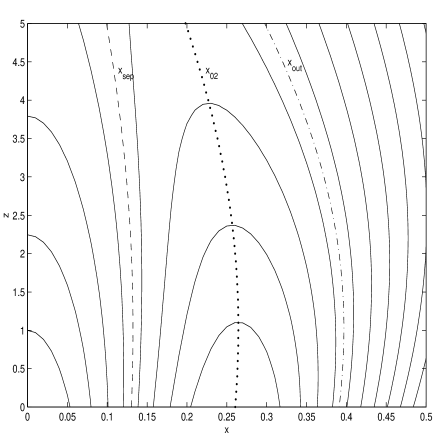
Figure 1: This picture illustrates the right side of our configuration (the left hand side can be derived from the symmetry assumption). The dashed ($--$) line corresponds to the separatrix $x_{sep}(z)$ between the streamers, the dotted ($\cdots$) line corresponds to the center of the outer streamer $x_{02}(z)$ and the dashdotted ($-\,\cdot$) line corresponds to the outer separatrix $x_{out}(z)$.

We choose $x_{0}=0$ to put the centre of the middle streamer on the $z$-axis. To calculate the separatrix between the middle and one of the outer streamer we use equation (11) with the form of $p(A)$ inside the middle streamer to obtain

$$x_{sep}=\sqrt{\frac{2}{p_{0}}}\frac{1}{c_{1}}\mbox{arctanh}\left(\sqrt{\frac{(p_{0}-k_{1}\exp(-c_{1}A_{s})}{p_{0}}}\right).$$ (21)

Note that both $p_{0}$ and $k_{1}$ may depend weakly on $z$.

If we call the centre of the outer streamer $x_{02}$, we can calculate this central field line relative to the separatrix field line again with equation (11), but this time using $p_{2}(A)$ and setting $x_{0}=x_{02}$:

$$x_{02}=x_{sep}+\sqrt{\frac{2}{p_{0}}}\frac{1}{c_{2}}\mbox{arctanh}\left(\sqrt{\frac{(p_{0}-k_{2}\exp(c_{2}A_{s})}{p_{0}}}\right)$$ (22)

If one takes into consideration that $p_{1}(A_{s})=p_{2}(A_{s})$ and Equation (21) one finds:

$$x_{02} = \mbox{arctanh}\left(\sqrt{\frac{(p_{0}-k_{1}\exp(-c_{1}A_{s})}{p_{0}}}\right)\sqrt{\frac{2}{p_{0}}}\left(\frac{1}{c_{1}}+\frac{1}{c_{2}}\right)$$

$$= \mbox{arctanh}\left(\sqrt{\frac{(p_{0}-k_{2}\exp(c_{2}A_{s})}{p_{0}}}\right)\sqrt{\frac{2}{p_{0}}}\left(\frac{1}{c_{1}}+\frac{1}{c_{2}}\right)$$

A sketch of the whole structure is shown in Figure 1.

We can now calculate $A$, $B_{z}$, $B_{x}$, $p$ and $j_{y}$ as functions of $x$ and $z$ from the Equations (13), (14), (15), (16) and (17) and by using the symmetry properties of these quantities. As an input we need the total pressure $p_{0}(z)$ which is the same in all three streamers, the parameters $c_{1}$, $c_{2}$ and $k_{1}$ and $k_{2}$. If gravitation is included, $k_{1}$ and $k_{2}$ may depend weakly on $z$, but could be different if we allow different temperatures inside the streamers.

2.4 Inclusion of flow

The method as outlined so far neglects that coronal streamers are the source regions of the slow solar wind. It is an open question if a stationary slow solar wind component exists or whether the slow solar wind is the result of many small eruptions. Recent observations (Schwenn and Inhester, private communication 1997) seem to favour the second alternative. If that is true, a steady state model providing the start configuration for a time-dependent computation of the eruption process need not include the flow, at least not near the symmetry plane. Nevertheless we want to show how a stationary plasma flow can be included in our model. It may be relevant for the open field regions at larger distances from the ecliptic, to which we confine the flow.

The inclusion of plasma flow into the asymptotic expansion procedure has been carried out for both incompressible Gebhardt (1989); Birn (1991) and compressible flow Birn (1992); Young and Hameiri (1992). There are three critical points in the solar wind: The slow magnetosonic point $v_{s}$, the Alfvén point $v_{A}$ and the fast magnetosonic point $v_{f}$ with $v_{s}<v_{A}<v_{f}$ for the coronal plasma. If one assumes that the flow velocity at the basis of the corona is less than $v_{s}$ the solar wind has to pass through all these critical points. Birn Birn (1992) showed that in stretched configurations the total pressure function $p_{0}(z)$ is related to the flow velocity. For $v<v_{s}$ the flow velocity decreases with decreasing $p_{0}(z)$ and for $v>v_{s}$ the flow velocity increases with decreasing $p_{0}(z)$. As it is necessary that $p_{0}(z)$ decreases with respect to $z$ to get closed arcade structures, the solar wind velocity should have a minimum at the helmet streamer cusp. This result is of course only valid if a stationary slow solar wind exists. The assumption of incompressible flow in the solar wind, however, cannot be justified in a strict sense, because generally gravity is not negligible. Since in the paper our main emphasis is placed on closed structures without directed flow, this model assumption does not influence our conclusions significantly. (In fact, all our explicit examples are structures without flow.) We note that the above mentioned variation of the solar wind velocity remains qualitative valid, if one neglects gravity and assumes incompressible flow. We will assume that the flow is purely field-aligned and since we will not extend our solution to the first critical point, we will for simplicity make the assumption of the flow being incompressible and subalfvenic.

We mention that, as a useful nice property, such stationary solutions with flow, can be directly calculated by transformation from static solutions Gebhardt and Kiessling (1992). Here we follow the approach developed in Birn Birn (1991). Equation (10) is then substituted by:

$$\frac{\partial A}{\partial x}=\pm\sqrt{\frac{2\left(p_{0}-p(A)\right)}{1-M_{A}^{2}(A)}}$$ (24)

where $M_{A}(A)$ is the Alfvén Mach number defined by $M_{A}=v/v_{A}$, where $v_{A}=B/\sqrt{\mu_{0}\rho}$ is the Alfvén velocity. Note that for incompressible flow both the Alfvén Mach number and the plasma density are constant along open field lines.

To extend the method outlined so far to include flow on open field lines, we have to define a second separatrix field line $A_{v}$ between the regions of open and closed magnetic flux. Since there shall be no flow in the closed field line regions, we choose $M_{A}(A)=0$ on the left hand side of the separatrix and $0<M_{A}(A)<1$ (subalfvénic flow) on the right hand of the separatrix. In the special case $M_{A}=\mbox{constant}$ we find with equation (24) that one can easily include incompressible subalfvenic plasma flow ($M_{A}<1$), if we replace the term $(x-x_{0})$ in the static theory by $(x-x_{0})/\sqrt{1-M_{A}^{2}}$. The location of the separatrix field line $A_{v}$ could be calculated by a similar procedure as the inner separatrix, but it is more convenient to choose it to be at the same distance from the centre of the outer streamer as the inner separatrix so that we have a symmetric situation again and one finds $A_{v}=A_{s}$. We remark that this condition is necessary if one investigates configurations with a cusp structure. One can then calculate the shape of the separatrix defined by $x_{out}(z)$ simply from $x_{out}(z)=2x_{02}(z)-x_{sep}(z)$ (see Figure 1 for illustration).

2.5 Inclusion of magnetic shear

It is possible to extend our method and include magnetic shear writing ${\bf B}$ as:

$${\bf B}(x,z)=\nabla A(x,z)\times\vec{e}_{y}+B_{y}(x,z)\vec{e}_{y}$$ (25)

Using the $y$ component of equation (1) one finds $B_{y}=B_{y}(A(x,z))$ and instead of (7) we get:

$$-\Delta A=\frac{\partial}{\partial A}\left(\Pi(A,\Psi)\right)$$ (26)

with

$$\Pi(A,\Psi)=\Pi(A,z)=k(z)p(A)+\frac{B_{y}^{2}(A)}{2}.$$

Using the method of asymptotic expansion we get:

$$x-x_{0}=\int_{A_{0}}^{A}\frac{dA}{\sqrt{2\left(p_{0}(z)-\Pi(A,z)\right)}}$$ (27)

We remark that the reason for magnetic shear should be a displacement of magnetic foot points and that only closed field lines will be sheared. We assume $B_{y}(A)\propto\exp(dA)$ for mathematical simplicity. In general we cannot solve equation (27) analytically. This is only possible if we choose the special case $d=\frac{c}{2}$ which we will do to illustrate the effect of magnetic shear. Then we get:

$$\Pi(A,z)=\left(k(z)+\frac{\lambda^{2}}{2}\right)\exp(cA)$$ (28)

and we can easily include magnetic shear by substituting $k(z)$ by $k(z)+\frac{\lambda^{2}}{2}$ in equation (13). It is possible to investigate other values ($c\not=2d$) numerically, but one can see the main effect of magnetic shear already in this special case.

We calculate triple structures analogous to the method without shear and substitute $p(A,z)$ by $\Pi(A,z)$. We have to consider shear only on closed field lines. We use $\Pi_{1}(A)=\left(k(z)+\frac{\lambda^{2}}{2}\right)\exp(-c_{1}A)$ in the middle streamer, $\Pi_{2}(A)=\exp(-(c_{1}+c_{2})A_{s})\left(k(z)+\frac{\lambda^{2}}{2}\right)\exp(c_{2}A)$ in the outer streamers and $\Pi_{3}(A)=\exp(-(c_{1}+c_{2})A_{s})k(z)\exp(c_{2}A)$ on open field lines. Thus there is a jump in $\Pi$ and a corresponding jump in the magnetic field at the boundary between outer streamers and open field lines and consequently there is a thin current sheet. Unlike the calculations on closed field lines one cannot fix $\Pi_{3}(A_{0})=p_{0}$. Instead of (11) one has to use:

$$x-x_{0}=\int_{A_{v}}^{A}\frac{dA}{\sqrt{2(p_{0}-\Pi_{3}(A))}}$$ (29)

where $A_{v}$ is the value of the last closed field line (boundary field line between open and closed regions). One finds $A_{v}=A_{s}$ for configurations with cusp structure.

We remark that violating the condition $\Pi_{1}(A_{s})=\Pi_{2}(A_{s})$ could still make sense. For example, one could use $P_{1}(A_{s})=P_{2}(A_{s})$ but $B_{y1}(A_{s})\not=B_{y2}(A_{s})$. Of course this mismatch in the value of $\Pi$ would have to be compensated by a corresponding mismatch in $B_{z}$ and this would lead to additional current sheets between the middle and the outer streamers.

2.6 Spherical coordinates

In this subsection we formulate the method in spherical coordinates $(r,\theta,\phi)$, which are more realistic to describe the solar corona on scales comparable to or larger than a solar radius. We assume static $({\bf v}=0)$ configurations and do not consider spatial variation in the $\phi$-direction $(\frac{\partial}{\partial\phi}=0)$. Thus we can present the magnetic field as:

$$B_{r} = \frac{1}{r^{2}\sin\theta}\frac{\partial\xi}{\partial\theta}$$

$$B_{\theta} = -\frac{1}{r\sin\theta}\frac{\partial\xi}{\partial r}$$

$$B_{\phi} = B_{\phi}(r,\theta)$$ (30)

Here $\xi$ is the flux function in spherical coordinates. We remark that in spherical coordinates the flux function is not identical with a component of the magnetic vector potential. One finds $\xi=r\sin(\theta)A_{\phi}$, where $A_{\phi}$ is the $\phi$-component of the vector potential ${\bf A}$. We find from (1) that $\xi(r,\theta)$ has to obey the equation:

$$\frac{\partial^{2}\xi}{\partial r^{2}}+\frac{\sin\theta}{r^{2}}\frac{\partial}{\partial\theta}\left(\frac{1}{\sin\theta}\frac{\partial\xi}{\partial\theta}\right)=-r^{2}\sin^{2}\theta\frac{\partial P(\xi,\Psi)}{\partial\xi}-\frac{1}{2}\frac{\partial f^{2}(\xi)}{\partial\xi}$$ (31)

where $f(\xi)=r\sin\theta B_{\phi}$ is constant on field lines. With the assumption of a constant temperature and because $\Psi=\Psi(r)$ one finds:

$$P(\xi,\Psi)=k(r)p(\xi)$$ (32)

with $k(r)=\exp(-(\Psi(r)-\Psi(0))/\mbox{R}T)$.

We assume that the magnetic field perpendicular to the photosphere $B_{r}$ is much larger than the parallel component $B_{\theta}$. For simplicity we do not consider magnetic shear here $(B_{\phi}=0)$. Stretched configurations are characterized by

$$\frac{1}{r^{2}}\frac{\partial}{\partial\theta}=O(1)\Rightarrow B_{r}=O(1)\quad\frac{1}{r}\frac{\partial}{\partial r}=O(\epsilon)\ll 1\Rightarrow B_{\theta}=O(\epsilon)$$

This approximation is valid for configurations close to the equatorial plane ($\theta=\frac{\pi}{2}$) and $r^{2}p_{0}(r)$ has to vary only slowly with respect to $r$. The second condition limits the outer boundary of our model corona to a few solar radii. As the observed configurations are indeed concentrated near the equatorial plane and the closed streamer field lines seem to be radially bounded to a few (about $2-4$) solar radii, our asymptotic model should describe these configurations approximately correct.

If we neglect terms of the order $\epsilon^{2}$ in Eq. (31) we obtain after one integration with respect to $\theta$:

$$\frac{\partial\xi}{\partial\theta}=^{+}_{-}r^{2}\sin(\theta)\sqrt{2(p_{0}(r)-k(r)p(\xi))}$$ (33)

We use (analogous to our calculations in Cartesian geometry) $p(\xi)=\exp(c\xi)$ and solve this differential equation by separation. Instead of (13) we get:

$$\xi(r,\theta)=\frac{\log(p_{0}(r))-\log(k(r)-2\log(\cosh(c\sqrt{\frac{p_{0}}{2}}r^{2}\left(\cos(\theta)-\cos(\theta_{0})\right))}{c}$$ (34)

We remark that one cannot find a one dimensional solution of equation (31) with $\xi=\xi(\theta)$ like in Cartesian geometry. Thus no analogy to the Harris sheet in Cartesian geometry exists in spherical coordinates.

To calculate triple structures in spherical geometry one uses a similar procedure as described for Cartesian geometry. We choose $\theta_{0}=\frac{\pi}{2}\Rightarrow\sin\theta_{0}=0$ to put the centre of the middle streamer and calculate the separatrix field line analogous to (21) and get:

$$\cos(\theta_{sep})=r^{2}\sqrt{\frac{2}{p_{0}}}\frac{1}{c_{1}}\mbox{arctanh}\left(\sqrt{\frac{(p_{0}-k_{1}\exp(-c_{1}A_{s})}{p_{0}}}\right)$$ (35)

If we call the center of the outer streamer $\theta_{02}$ we get analogous to our calculations in Cartesian geometry:

$$\cos(\theta_{02}) = r^{2}\sqrt{\frac{2}{p_{0}}}\left(\frac{1}{c_{1}}+\frac{1}{c_{2}}\right)\mbox{arctanh}\left(\sqrt{\frac{(p_{0}-k_{1}\exp(-c_{1}A_{s})}{p_{0}}}\right)$$ (36)

$$= r^{2}\sqrt{\frac{2}{p_{0}}}\left(\frac{1}{c_{1}}+\frac{1}{c_{2}}\right)\mbox{arctanh}\left(\sqrt{\frac{(p_{0}-k_{2}\exp(-c_{2}A_{s})}{p_{0}}}\right)$$

The quantities $\xi$, $B_{r}$, $B_{\theta}$, $p$, $j_{\phi}$ can then be calculated as functions of $r$ and $\theta$ in the usual way.

3 Results

3.1 Static solutions in Cartesian geometry without gravitation

Table 1: Parameter sets used to calculate the solutions presented in Figure 2

Solution	$s_{1}$	$s_{2}$	$s_{3}$	$c_{1}$	$c_{2}$	$A_{s}$
a)	0.8	0.4	0.2	15.0	15.0	0.1
b)	0.8	0.4	0.2	15.0	15.0	0.08
c)	0.8	0.4	0.2	20.0	20.0	0.12
d)	0.8	0.4	0.2	10.0	30.0	0.12
e)	0.8	0.4	0.2	30.0	12.0	0.04
f)	0.8	1.2	0.2	15.0	15.0	0.12

We first give a few examples for triple streamers calculated with our model to illustrate the influence of the different functions and parameters on the structure of the solutions. To calculate a solution we have to specify the functions $p_{0}(z)$ and $k_{1}(z)$ and the parameters $c_{1}$, $c_{2}$ and $A_{s}$. In the first examples we neglect the effect of plasma flow and of the solar gravitation which gives $k_{1}(z)=1$. Our solutions are confined within the boundaries $x=-0.5..0.5$ and $z=0..5$ corresponding to one solar radius in the $x$ direction and five solar radii in the $z$ direction. We use symmetry with respect to the $z$ axis.

We prescribe the total pressure by $p_{0}(z)=s_{1}\exp(-s_{2}z)+s_{3}$. Within our model $A(x,z)$ depends only parametrically on $z$ by $p_{0}(z)$ and so the exact form of $p_{0}(z)$ has not too much influence on the configuration as long as its general properties are similar. One important property of $p_{0}(z)$ is that it has to be a monotonically decreasing function of $z$ to obtain singly connected closed field line regions. Physically one can identify the total pressure on the $x$-axis with the sum of the magnetic pressure $B^{2}/2$ on open field lines outside the helmet streamer and a homogeneous plasma pressure of the solar wind.

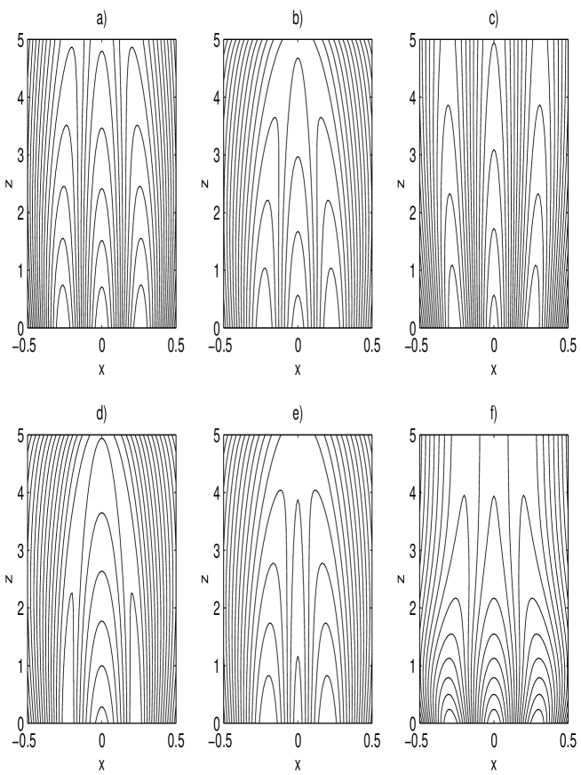
Figure 2: Magnetic field lines (contourplot of $A(x,z)$) for triple helmet streamers (see text)

In Figure 2 we show field line plots of six solutions calculated for different sets of parameters which are summarized in Table 1. In Figure 2a) - 2c) we investigate the influence of the location of the separatrix field line on the solutions structure, whereas $p_{0}$ is kept fixed and the parameters $c_{1}$ and $c_{2}$ are fixed to a value of $15.0$ in a) and b) whereas we used $c_{1}=c_{2}=20.0$ in c) which leads to thinner configurations. In these cases all three streamers have exactly the same width though the width itself varies. In Figure 2a) the separatrix is a straight line giving rise to parallel streamers. In Figure 2b) the separatrix has been moved closer to the centre of the structure and the three streamers converge, whereas in Figure 2c) the separatrix has been moved further out giving rise to diverging streamers.

In Figure 2d) we have decreased the value of $c_{1}$ to $10.0$ and increased the value of $c_{2}$ to $30.0$. Also the value for $A_{s}$ has been increased. The effect is that the central streamer now contains more magnetic flux than the outer streamers and is wider in the $x$-direction. In Figure 2e) this effect has been reversed by making $c_{2}$ smaller than $c_{1}$. It is obvious that now the outer streamers are wider than the central streamer.

Finally, in Figure 2f) we have varied the total pressure $p_{0}(z)$ by increasing the parameter $s_{2}$ to $1.2$ resulting in a faster decrease of $p_{0}$ with $z$. One notices that the closed field line regions (which we define here loosely as those field lines not crossing the upper boundary) has shrunk and that the whole structure has a much slimmer appearance for large $z$.

Table 2: Parameter sets used to calculate the solutions presented in Figure 3

Solution	$a$	$b$	$n$	$z_{\mbox{\tiny cusp}}$	$c_{1}$	$c_{2}$	$A_{s}$
a)	0.8	0.2	3.0	4.0	15.0	15.0	0.1073
b)	0.8	0.2	4.0	4.0	10.0	25.0	0.1609
c)	0.8	0.2	6.0	4.0	25.0	12.0	0.0644

In a next step we use our model to describe helmet streamer configurations with a cusp. Up to now we have not given a radial boundary of the closed magnetic field lines. Now we define such a point at $x=0$, $z=z_{\mbox{\tiny cusp}}$ which defines the last closed field line.

We use as a function for the total pressure:

$$p_{0}(z)=\left\{\begin{array}[]{r@{\quad\mbox{for}\quad}l}a(\frac{z_{\mbox{\tiny cusp}}-z}{z_{\mbox{{\tiny cusp}}}})^{n}+b&z\leq z_{\mbox{\tiny cusp}}\\ b&z>z_{\mbox{\tiny cusp}}\end{array}\right.$$ (37)

Field line plots for three different sets of parameters are shown in Figure 3. The parameter sets used are listed in Table 2. It can be seen that the effect of changing the parameters $c_{1}$ and $c_{2}$ stays the same as in the case without cusp. An increase of the exponent $n$ leads to a stronger decrease of $p_{0}(z)$ as the cusp point is approached from below and this leads to a sharper cusp structure.

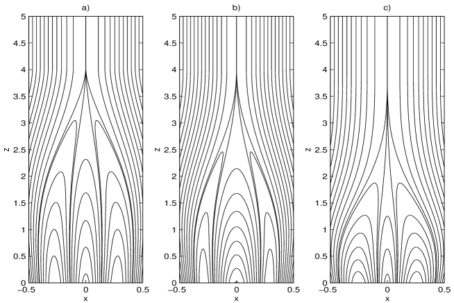
Figure 3: Magnetic field lines (contourplot of $A(x,z)$) for triple helmet streamers with cusp (see text for discussion).

These examples illustrate the flexibility of our model. One can describe different types of triple helmet streamers by specifying the free parameters in the general solutions.

3.2 Static solutions in Cartesian Geometry Including Magnetic Shear and Gravitation

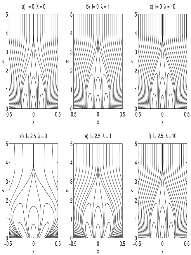
Figure 4: Magnetic field lines (contourplot of $A(x,z)$) for triple helmet streamers. In the upper pictures b) and c) we included magnetic shear and in the lower pictures we additionally investigated the effect of gravitation.

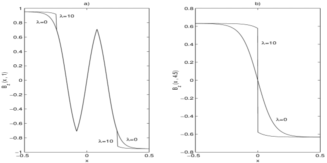
Figure 5: The main magnetic field component $B_{z}(x)$ without ($\lambda=0$) and with $(\lambda^{2}=10)$ shear: a) Below the cusp $(z=1.0)$; b) above the cusp ($z=4.5$).

In this section we investigate the influence of the solar gravitational field on the structure of the solutions. Though we are still calculating in Cartesian geometry we will not take the gravitational force to be constant as it is usually done in Cartesian geometry if the length scale under consideration is much smaller than a solar radius (e.g. Zwingmann 1987; Platt and Neukirch 1994), but use the more appropriate potential $\Psi=\Psi(z)=-\frac{GM_{s}}{z+R_{s}}$. Together with the assumption of constant temperature we get:

$$k(z)=\exp\left(-\frac{l}{R_{s}}\right)\cdot\exp\left(\frac{l}{z+R_{s}}\right)$$ (38)

where $G$ is the constant of gravitation, $M_{s}$ the solar mass, $R_{s}$ the solar radius and $l=\frac{GM_{s}}{RT}$. Under the assumption of a pure hydrogen plasma and a constant temperature of $3\cdot 10^{6}$ K one finds $l\approx 7.5$ corresponding to $7.5\,R_{s}$. One difficulty of the method in Cartesian geometry is that $k(z)$ must decrease more slowly with respect to $z$ than $p_{0}(z)$ because otherwise one cannot find arcade type solutions. This is difficult to achieve with a realistic value of $l$, but since we only want to investigate the qualitative effect of gravitation on the solution we use the unrealistic but mathematically more convenient value $l=2.5$. We remark that this problem is alleviated in spherical geometry which is more realistic anyway (see section 3.3)

The inclusion of shear only makes sense on closed field lines. As we have a well defined boundary between open and closed regions only in solutions with cusp structure, we only investigate such configurations here. In Figure 4 we fix the parameters $c_{1}=c_{2}=25.0,z_{cusp}=4.0,a=0.8,n=4.0,b=0.2$ and use for the total pressure:

$$p_{0}(z)=\left\{\begin{array}[]{r@{\quad\mbox{for}\quad}l}\left(k(z)+\frac{\lambda^{2}}{2}\right)\left[a\left(\frac{z_{\mbox{\tiny cusp}}-z}{z_{\mbox{{\tiny cusp}}}}\right)^{n}+b\right]&z\leq z_{\mbox{\tiny cusp}}\\ b\left(k(z)+\frac{\lambda^{2}}{2}\right)&z>z_{\mbox{\tiny cusp}}\end{array}\right.$$ (39)

The factor $\left(k(z)+\frac{\lambda^{2}}{2}\right)$ can be used to fix the normal component of the magnetic field at the solar surface, which we could use as a boundary condition.

The main effect of magnetic shear is that there is a jump in the magnetic field and consequently a thin current sheet between the closed and open field lines. Indications of such a current sheet are also found in recent observations Schwenn et al. (1997). In Figure 5a) we plot $B_{z}$ as a function of $x$ at the height $z=1$ for the same parameters as in Figures 4a) and c).

If we do not include shear the structure above the helmet streamer cusp $z>z_{cusp}$ becomes equivalent to a Harris sheet and $B_{z}$ goes smoothly through zero in the center of the configuration. The inclusion of shear on closed field lines leads to a jump in $B_{z}$ from a positive to a negative value in the center of the whole configuration (see figure 5 b)). This causes a thin current sheet, which is more pronounced than the current sheet at the outer boundary of the streamer configuration below the cusp. This current sheet corresponds to the heliospheric current sheet. The effect can clearly be seen in Figure 4. In the Figures 4b) and c) we included magnetic shear and in c) the shear is stronger than in b) leading to a larger jump in $B_{z}$. This can be seen in the contourplot of $A$ as the field line density is much higher in the center above the cusp in Figure 4c) than in b). In the lower panel (Figure 4d)-f)) we investigated the same configurations as in the upper pictures but included gravitation. One can see that without shear (Figure 4d)), the configuration gets wider with increasing $z$. (If one uses the realistic value $l=7.5$ instead of $l=2.5$ the configuration will become unrealistically wide without shear.) The inclusion of shear reduces this effect and if one investigates force free configurations $\left(\frac{\partial P(A)}{\partial A}=\nabla P=0\right)$ or nearly force free solutions $\left(\frac{\partial B_{y}^{2}(A)}{\partial A}\gg\frac{\partial P(A)}{\partial A}\right)$ which is accomplished in c) and f) the effect of gravitation vanishes.

3.3 Solutions in spherical geometry

Now we present some example solutions of helmet streamer configurations in spherical coordinates. This geometry is of course more realistic to describe the coronal magnetic field on large scales. In this section we also include the influence of the solar gravitational field on the structure of the solutions from the beginning. With $\Psi=\Psi(r)=-\frac{GM_{s}}{r}$ we get as in Cartesian geometry (see Section 3.2)

$$k(r)=\exp\left(-\frac{l}{R_{s}}\right)\cdot\exp\left(\frac{l}{r}\right)$$ (40)

Here we use the realistic value $l=7.5$.

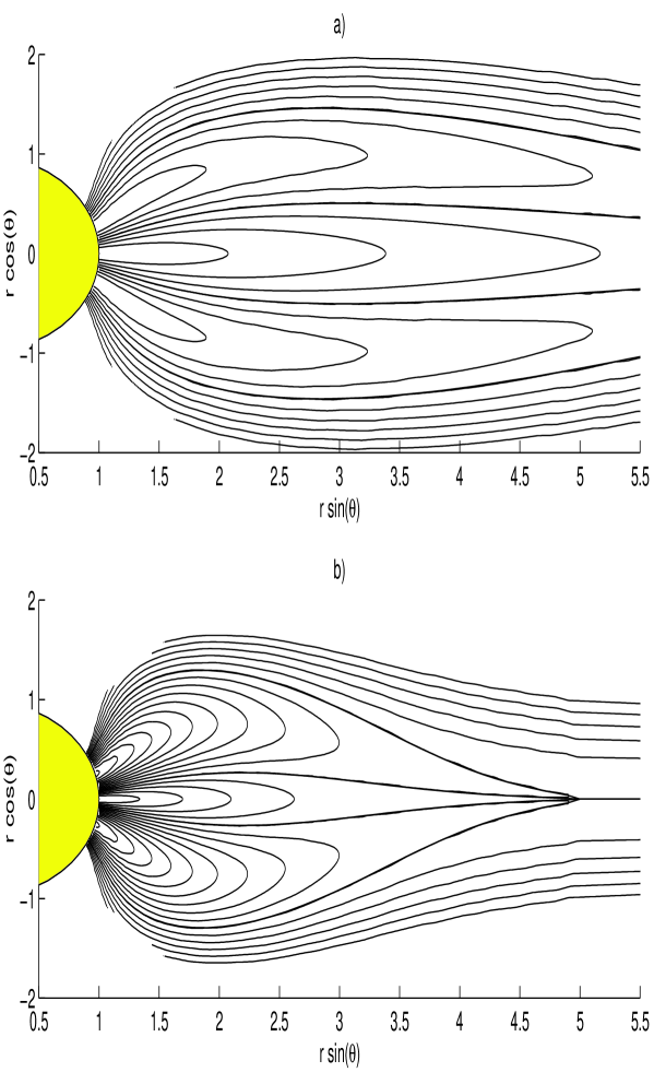
Figure 6: Magnetic field lines (contourplot of $\xi(r,\theta)$) for triple helmet streamers in spherical geometry (see text)

In Figure 6a) we show a field line plot of a solution in which we prescribed the total pressure as $p_{0}(r)=k(r)\left[s_{1}\exp(-s_{2}(r-1))+s_{3}\right]$ and used the same parameters as in Figure 2a) (see Table 1, case a). Thus $p_{0}(r)/k(r)$ varies in the same way as $p_{0}(z)$ in the Cartesian case without gravitation. The effects of the different geometry show up as a bending of the out streamers towards the equatorial plane.

In Figure 6b) (see Table 2, case b) we present a solution with cusp structure in spherical geometry with the total pressure

$$p_{0}(r)=\left\{\begin{array}[]{r@{\quad\mbox{for}\quad}l}k(r)\left[a(\frac{r_{\mbox{\tiny cusp}}-r+1}{r_{\mbox{{\tiny cusp}}}})^{n}+b\right]&r\leq r_{\mbox{\tiny cusp}}\\ k(r)b&r>r_{\mbox{\tiny cusp}}\end{array}\right.$$ (41)

and use the same parameters as in Figure 3c). Again the bending of the outer streamers is obvious.

We remark that prescribing the parameters $c_{1},c_{2}$ and $p_{0}(R_{s})$ is equivalent to prescribing the normal component of the magnetic field at the solar surface. This property of the solutions could be used to match measured magnetic fields and generate the corresponding streamer structure.

4 Conclusions and outlook

We have developed a comparatively simple procedure based on the method of asymptotic expansion to calculate equilibria of triple helmet streamer structures. The procedure represents a generalization of the asymptotic expansion method used in the theory of magnetotail equilibria Schindler (1972); Birn et al. (1975); Schindler und Birn (1982). We have applied this procedure to the calculation of stationary states of triple helmet streamers under various conditions and investigated the dependence of the solution properties on the model parameters, the influence of the solar gravitational field, the inclusion of field aligned flow and on the basic geometry used.

As a next step we plan to use the calculated configurations as start equilibria for MHD simulations. These simulations will answer the question of stability which we did not address in this paper and provide important insights into possible mechanisms of eruptive phenomena in the solar atmosphere, especially those connected with a triple structure of the solar corona. The simulations should have relevance both for huge coronal mass ejections and very small but frequent eruptions which may represent the source mechanism of the slow solar wind.

Middle Streamer

With $c=-c_{1}$, $k=k_{1}$ and $x_{0}=0$ one finds:

$$\frac{\partial A}{\partial p_{0}}=\frac{1}{c_{1}}\left(-\frac{1}{p_{0}}+\frac{c_{1}x}{\sqrt{2p_{0}}}\tanh(\sqrt{\frac{p_{0}}{2}}c_{1}x)\right)$$

$$\frac{\partial A}{\partial k_{1}}=\frac{1}{k_{1}c_{1}}$$

Outer Streamers

With $c=c_{2}$, $k=k_{2}$ and $x_{0}=x_{02}$ (see equation(2.3)) one finds:

$$\frac{\partial A}{\partial p_{0}} = \frac{\left(2\sqrt{p_{0}}\sqrt{\alpha_{1}}c_{1}\sqrt{\frac{1}{p_{0}}}\cosh(\alpha_{2})+\sinh(\alpha_{2})p_{0}\sqrt{2}\sqrt{\alpha_{1}}\sqrt{\frac{1}{p_{0}}}xc_{1}c_{2}-2\sinh(\alpha_{2})(c_{1}+c_{2})\right)}{2\left(p_{0}^{3/2}\sqrt{\alpha_{1}}c_{1}\sqrt{\frac{1}{p_{0}}}\cosh(\alpha_{2})c_{2}\right)}$$

$$\frac{\partial A}{\partial k_{2}}=\hbox to0.0pt{$\displaystyle\left({\vrule height=8.39996pt,width=0.0pt,depth=8.39996pt}\right.\!\!{\rm sinh}(\,{\rm\alpha_{2}}\,)\,{\it p_{0}}\,\sqrt{{\displaystyle\frac{1}{{\it p_{0}}}}}\,{\it c_{2}}+{\rm sinh}(\,{\rm\alpha_{2}}\,)\,{\it p_{0}}\,\sqrt{{\displaystyle\frac{1}{{\it p_{0}}}}}\,{\it c_{1}}$\hss}$$

$$\mbox{}-\sqrt{{\it p_{0}}}\,\sqrt{{\rm\alpha_{1}}}\,{\it c_{1}}\,{\rm cosh}(\,{\rm\alpha_{2}}\,)\!\!\left.{\vrule height=8.39996pt,width=0.0pt,depth=8.39996pt}\right)\left/{\vrule height=4.10004pt,width=0.0pt,depth=4.10004pt}\right.\!\!\left({\vrule height=4.10004pt,width=0.0pt,depth=4.10004pt}\right.\!\!\,\sqrt{{\it p_{0}}}\,\sqrt{{\rm\alpha_{1}}}\,{\it k_{2}}\,{\it c_{1}}\,{\rm cosh}(\,{\rm\alpha_{2}}\,){\it c_{2}}\,\!\!\left.{\vrule height=4.10004pt,width=0.0pt,depth=4.10004pt}\right)$$

Therefore we used as abbreviations:

$$\alpha_{1}:={\displaystyle\frac{p_{0}-k_{2}\,\exp(c_{2}\,A_{s})}{p_{0}}}$$

$${\rm\alpha_{2}}:={\displaystyle\frac{1}{2}}\sqrt{{\it p_{0}}}\left({\vrule height=8.39996pt,width=0.0pt,depth=8.39996pt}\right.\!\!-\sqrt{2}\,{x}\,{\it c_{1}}\,{\it c_{2}}+2\,{\rm arctanh}\left(\!\,\sqrt{{\rm\alpha_{1}}}\,\!\right)\,\sqrt{{\displaystyle\frac{1}{{\it p_{0}}}}}\,{\it c_{2}}$$

$$\mbox{}+2\,{\rm arctanh}\left(\!\,\sqrt{{\rm\alpha_{1}}}\,\!\right)\,\sqrt{{\displaystyle\frac{1}{{\it p_{0}}}}}\,{\it c_{1}}\!\!\left.{\vrule height=8.39996pt,width=0.0pt,depth=8.39996pt}\right)\left/{\vrule height=3.69995pt,width=0.0pt,depth=3.69995pt}\right.\!\!{\it c_{1}}$$

References

- Bavassano et al. (1997) Bavassano, B., Woo, R. and Bruno, R.: 1997 Geophys. Res. Lett. 24, 1655.
- Birk and Otto (1997) Birk, G.T. and Otto, A.: 1997, Adv. Space Res. 19, 1879.
- Birk et al. (1997) Birk, G.T., Konz, C. and Otto, A.: 1997, Phys. Plasmas, in press
- Birn (1991) Birn, J.: 1991, Phys. Fluids B 3, 479.
- Birn (1992) Birn, J.: 1992, J. Geophys. Res. 97, 16817.
- Birn and Schindler (1981) Birn, J. and Schindler, K.: 1981, in Priest, E.R. (Ed.) Solar Flare Magnetohydrodynamics; Gordon and Breach, New York, 337.
- Birn et al. (1978) Birn, J., Goldstein, H. and Schindler, K.: 1978, Solar Phys. 57, 81.
- Birn et al. (1975) Birn, J., Sommer, R. and Schindler, K.: 1975, Astrophys. Space Sci. 35, 389.
- Crooker et al. (1993) Crooker, N.U.,Siscoe, G.L., Shodan, S., Webb, D.F., Gosling, J.T. and Smith, E.J.: 1993, J. Geophys. Res. 98, 9371.
- Cuperman et al. (1995) Cuperman, S., Bruma, C., Dryer, M. and Semel, M.: 1995, Astron. Astrophys. 299, 389.
- Cuperman et al. (1992) Cuperman, S., Detman, T.R., Bruma, C. and Dryer, M.: 1992, Astron. Astrophys. 265, 785.
- Cuperman et al. (1990) Cuperman, S., Ofman, L. and Dryer, M.: 1990, Astrophys. J. 350, 846.
- Dahlburg and Karpen (1995) Dahlburg, R.B. and Karpen, J.T.: 1995, J. Geophys. Res. 100, 23489.
- Gebhardt (1989) Gebhardt, U.: 1989, Diplom Thesis, Ruhr-Universität Bochum.
- Gebhardt and Kiessling (1992) Gebhardt, U. and Kiessling, M.K-H.: 1992, Phys. Fluids B 4, 1689.
- Hundhausen (1995) Hundhausen, A.J.: 1995, in K. Strong, J. Saba and B, Haisch (eds.), The Many Faces of the Sun, in press.
- Koutchmy and Livshits (1992) Koutchmy, S. and Livshits, M.: 1992, Space Sci. Rev. 61, 393.
- Low (1975) Low, B.C.: 1975, Astrophys. J. 197, 251.
- Low (1980) Low, B.C.: 1980, Solar Phys. 65, 147.
- Otto and Birk (1992) Otto, A. and Birk, G.T.:1991, Phys. Fluids B 4, 3811.
- Platt and Neukirch (1994) Platt, U. and Neukirch, T.: 1994, Solar Phys. 153, 287.
- Pneuman and Kopp (1971) Pneuman, G.W. and Kopp, R.A.: 1971, Solar Phys. 18, 258.
- Schindler (1972) Schindler, K.: 1972, in B.M. McCormac (ed.), Earth’s Magnetospheric Processes, D. Reidel Publ. Comp., Dordrecht 1972, p.200
- Schindler und Birn (1982) Schindler, K. and Birn, J.: 1982, J. Geophys. Res. 87, 2263.
- Schwenn et al. (1997) Schwenn, R., Inhester, B., Plunkett, S.P., Epple, A., Podlipnik, B. et al.: 1997 Solar Phys., in press .
- Wang et al. (1993) Wang, A.-H., Wu, S.T., Suess, S.T. and Poletto, G.: 1993, Solar Phys. 147, 55.
- Wang et al. (1997) Wang, S., Liu, Y.F. and Zheng, H.N.: 1997, Solar Phys. 173, 409.
- Wiegelmann (1997) Wiegelmann, T.: 1997, Physica Scripta, in press.
- Wiegelmann and Schindler (1995) Wiegelmann, T. and Schindler, K.: 1995, Geophys. Res. Lett. 22, 2057.
- Woo et al. (1995) Woo, R., Armstrong, J.W., Bird, M.K. and Pätzold, M.: 1995, Astrophys. J. 449, L91.
- Wu et al. (1995) Wu, S.T., Guo, W.P. and Wang, J.F.: 1995, Solar Phys. 157, 325.
- Yan et al. (1994) Yan, M., Otto, A. Muzzell, D. and Lee, L.C.: 1994, J. Geophys. Res. 99, 8657.
- Young and Hameiri (1992) Young, R. and Hameiri, E.: 1992, J. Geophys. Res. 97, 16789.
- Zwingmann (1987) Zwingmann, W.: 1987, Solar Phys. 111, 309.