Dwarf Spheroidal Satellite Galaxies Without Dark Matter: Results From Two Different Numerical Techniques

Abstract

Self-consistent simulations of the dynamical evolution of a low-mass satellite galaxy without dark matter are reported. The orbits have eccentricities $0.41\leq e\leq 0.96$ in a Galactic dark halo with a mass of $2.85\times 10^{12}\,{\rm M}_{\odot}$ and $4.5\times 10^{11}\,{\rm M}_{\odot}$. For the simulations, a particle-mesh code with nested sub-grids and a direct-summation N-body code running with the special purpose hardware device Grape are used. Initially, the satellite is spherical with an isotropic velocity distribution, and has a mass of $10^{7}\,M_{\odot}$. Simulations with $1.3\times 10^{5}$ up to $2\times 10^{6}$ satellite particles are performed. The calculations proceed for many orbital periods until well after the satellite disrupts.

In all cases the dynamical evolution converges to a remnant that contains roughly 1 per cent of the initial satellite mass. The stable remnant results from severe tidal shaping of the initial satellite. To an observer from Earth these remnants look strikingly similar to the Galactic dwarf spheroidal satellite galaxies. Their apparent mass-to-light ratios are very large despite the fact that they contain no dark matter.

These computations show that a remnant without dark matter displays larger line-of-sight velocity dispersions, $\sigma$, for more eccentric orbits, which is a result of projection onto the observational plane. Assuming they are not dark matter dominated, it follows that the Galactic dSph satellites with $\sigma>6$ km/s should have orbital eccentricities of $e>0.5$. Some remnants have sub-structure along the line-of-sight that may be apparent in the morphology of the horizontal branch.

1 Introduction

At least about ten dwarf spheroidal (dSph) galaxies are known to orbit the Milky Way at distances ranging from a few tens to a few hundred kpc. On the sky they are barely discernible stellar density enhancements. Some have internal substructure and appear flattened. Their velocity dispersions are similar to those seen in globular clusters and they have approximately the same stellar mass. However, they are about two orders of magnitude more extended. For spherical systems in virial equilibrium with an isotropic velocity dispersion, the overall mass of the system can be determined from the observed velocity dispersion. Comparing this ‘gravitational’ mass to the luminosity of the system determines the mass-to-light ratio, $M/L$ (in the following always given in solar units ${\rm M}_{\odot}/{\rm L}_{\odot}$). In the solar neighbourhood this ratio is $3<M/L<5$ (e.g. Tsujimoto et al. 1997). Values for $M/L$ of about 10 or larger are usually taken to imply the presence of dark matter in a stellar system. For the dSph satellites, $M/L$ values as large as a few hundred are inferred, implying that these systems may be completely dark matter dominated (for a review see Mateo 1997).

A careful compilation of the observed structural parameters and kinematical data for the Galactic dSph galaxies can be found in Irwin & Hatzidimitriou (1995). More general reviews are given by Ferguson & Binggeli (1994), Gallagher & Wyse (1994), Meylan & Prugniel (1994), Grebel (1997) and Da Costa (1997).

There are in principle two possibilities for achieving apparent high mass-to-light ratios without dark matter: Unresolved binary stars may inflate the measured velocity dispersion thus increasing $M/L$. However, this effect is not large enough for a reasonable population of binary systems (Hargreaves et al. 1996; Olszewski et al. 1996). Assuming Newtonian gravity is valid in dSph galaxies, an alternative may be that the assumption of virial equilibrium is violated: the satellite galaxies might be significantly perturbed by Galactic tides. The structural, kinematical and photometric data of the dSph satellites show correlations that may be interpreted to be the result of significant tidal shaping (Bellazzini, Fusi Pecci & Ferraro 1996). Extra-tidal stars indicate that most dSph satellites may be losing mass (Irwin & Hatzidimitriou 1995, Kuhn, Smith & Hawley 1996, Smith, Kuhn & Hawley 1997), and Burkert (1997) points out that, if the tidal radii derived from the Irwin & Hatzidimitriou (1995) profiles assuming King models are correct, then these radii are smaller than expected from the observed large $M/L$ values.

The “tidal scenario” has been studied in detail by a variety of authors: Oh et al. (1995) modelled the evolution of dSph galaxies on different orbits in a set of rigid spherical Galactic potentials. The satellites are represented by $10^{3}$ particles and are evolved using a softened direct N-body program over many orbital periods until disruption. Their work allows important insights into the tidal stability of such systems. Piatek & Pryor (1995) concentrate on one peri-galactic passage of a dSph galaxy in different rigid spherical Galactic potentials. Their satellite consists of $10^{4}$ particles and is modelled using a Treecode scheme. They find that a single peri-galactic passage cannot perturb a satellite significantly enough for an observer to measure a high $M/L$ ratio, reaching similar conclusions as Oh et al. (1995). Johnston, Spergel & Hernquist (1995), who apply their simulations to the dynamical evolution of the Sagittarius satellite galaxy, also arrive at similar conclusions.

Self-consistent simulations of the long-term evolution of a low-mass satellite galaxy on two different orbits and interacting with an extended Galactic dark halo are presented by Kroupa (1997; hereafter referred to as K97). The satellite consists of $3\times 10^{5}$ particles and the whole system is evolved applying a particle-mesh scheme with nested sub-grids, the aim being to study the system well after the satellite has mostly dissolved and to ‘observe’ its properties as it would be seen from Earth. The satellite is projected onto the sky and its brightness profile, line-of-sight velocity dispersion and apparent $M/L$ ratio are determined. These quantities can be directly compared to the observed values for Galactic dSph galaxies.

His main finding is that a remnant containing about 1 per cent of the initial satellite mass remains as a long-lived and distinguishable entity after the major disruption event. To an observer from Earth, this remnant looks strikingly similar to a dSph galaxy. The remnant consists of particles that have phase-space characteristics that reduce spreading along the orbit. That this is a possibility to be considered had been pointed out by Kuhn (1993). However, projection effects are also important. An observer who’s line-of-sight subtends a small angle with the orbital path of the remnant sees an apparently brighter satellite with internal sub-clumps and an inflated velocity dispersion. The flattened structure that may be apparent to the observer need not have a major axis that is oriented along the orbital path. The observer derives values for $(M/L)_{\rm obs}$ that are much larger than the true mass-to-light ratio $(M/L)_{\rm true}$ of the particles, because the object is far from virial equilibrium and has a velocity dispersion tensor that is significantly anisotropic.

The aim of the present study is to investigate if the conclusions of K97 can be arrived at when higher resolution simulations with more particles are used, and when a different numerical scheme altogether is employed. We thus hope to confirm that the high $M/L$ values of the Galactic dSph satellites can be explained without the need for dark matter. We furthermore suggest possible observational discriminants, and continue the analysis of the two snapshots studied in K97.

In addition to the particle-mesh method applied in K97 and here, we use a direct N-body integrator in connection with the special purpose hardware device Grape, which allows the integration of systems with $10^{5}$ or more particles. It is therefore a useful tool for studying the evolution of dSph galaxies in a Galactic dark halo.

Using two different numerical schemes enables us to determine where the models agree, i.e. which conclusions are firm, and also where they show deviations. This allows us to quantify uncertainties inherent to the numerical method, but we do not aim at an in-depth discussion of the detailed differences between the two numerical schemes. We will show that the general conclusions agree for both methods, and that they can both be used equivalently to explore further regions in parameter space. The simulations described here are part of an extensive study of parameter space to investigate which orbits and which assumption for the Galactic dark halo may lead to dSph-like objects on the sky. Detailed reports about this survey will be presented elsewhere.

In the next section we give a short introduction to the two numerical schemes applied here, followed by a description of the data analysis used to evaluate the simulations. Section 3 treats the initial conditions, and in Section 4 we discuss our results. Possible discriminants between dark-matter and tidal models are presented in Section 5. We conclude with Section 6.

2 Two Numerical Schemes and Data Analysis

A short description of both numerical schemes used for the simulations is provided in Sections 2.1 and 2.2, and the data reduction method is described in Section 2.3.

2.1 Direct Integration Scheme with GRAPE

Grape is a special purpose hardware device. Its name is an acronym for ‘GRAvity PipE’. The device solves Poisson’s and the force equations for a gravitational N-body system by direct summation on a specially designed chip, thus leading to a considerable speed-up (Sugimoto et al. 1990, Ebisuzaki et al. 1993). We use the currently distributed version, Grape-3AF, which contains 8 chips on one board and therefore can compute the forces on 8 particles in parallel. The board is connected via a standard VME interface to the host computer, in our case a SUN Sparcstation. C and FORTRAN libraries provide the software interface between the user’s program and the board. The computational speed of Grape-3AF is approximately $5\,$Gflops.

The force law is hardwired to be a Plummer law,

$${\bf F}_{i}\>=\>-G\sum_{j=1}^{N}\frac{m_{i}m_{j}({\bf r}_{i}-{\bf r}_{j})}{(|{\bf r}_{i}-{\bf r}_{j}|^{2}+\epsilon_{i}^{2})^{3/2}}\>.$$ (1)

Here $i$ is the index of the particle for which the force is calculated and $j$ enumerates the particles which exert the force; $\epsilon_{i}$ is the gravitational smoothing length of particle $i$; $G$, $m_{i}$ and $m_{j}$ are Newton’s constant and the particle masses, respectively. We chose all particles to have the same masses and smoothing lengths.

To increase speed, concessions in the accuracy of the force calculations had to be made: Grape internally works with a 20 bit fixed point number format for particle positions, with a 56 bit fixed point number format for the forces and a 14 bit logarithmic number format for the masses (Okumura et al. 1993). Conversion to and from this internal number representation is handled by the interface software. The number format limits the spatial resolution in a simulation and constrains the force accuracy. However, for collisionless N-body systems, the forces on a single particle need not be known to better than about one per cent. In that respect, Grape is comparable to the widely used Treecode schemes (e.g. Barnes & Hut 1986).

We utilise Grape by implementing the direct summation approach. This essentially involves two nested loops: an outer one over all particles for which forces are calculated, and an inner loop for the interaction of each of those with all other particles in the system. Therefore, the number of operations scales as ${\cal O}(N^{2})$ with the particle number $N$. Typically, this scaling law limits the particle number to a few thousand. However, Grape substitutes the inner loop and thus a considerable speed-up is gained. We furthermore implement variable time-steps and interpolate the particle accelerations when no new force calculations are needed within the required accuracy. Once the accelerations are obtained in each time-step, the particles are advanced using the leap-frog scheme. The satellite galaxy is described with $131\,072$ particles. To give an estimate for the computational time needed: a simulation with 5500 time-steps (e.g. the run Sat-M2 in Table 1) typically takes three days on a Sun Sparcstation with the Grape board.

2.2 SUPERBOX: A Particle-Mesh Code with Nested Sub-grids

Superbox is a conventional particle-mesh code (see e.g. Sellwood 1987) but allows high spatial resolution of density maxima by employing three levels of nested grids. Each active grid has $N_{\rm grid}=(2K)^{3}$ cells, where $K$ is a positive integer. The outermost, coarsest grid contains the local universe. The sub-grids of the two lower levels are positioned at the density maximum of a galaxy and follow its motion through the coarse outer grid. In principle any number of interacting galaxies can be treated. The force acting on each particle is obtained by first solving Poisson’s equation using the Fast Fourier Transform technique, and then by numerically differentiating the potential at the position of the particle. The leap-frog integration scheme is used to advance the particles along their orbits (for a brief description of the code see K97, a detailed account will be provided elsewhere).

For the present purpose, Superbox is used to simulate the interaction of two galaxies, namely of the Galactic dark halo and the satellite galaxy. Typically, $N_{\rm grid}=32^{3}$ cells per grid and in total $1.3\times 10^{6}$ particles are used. In addition, two simulations with $N_{\rm grid}=64^{3}$ cells on each level and in total $4\times 10^{6}\,$ particles are run to test the numerical resolution of Superbox. An 8000-time-step long simulation takes 5 CPU days on an IBM RISC/6000 350 workstation in the first case, and in the latter case it takes 55 CPU days on a SUN Sparcstation 10/514.

2.3 Data Evaluation

The model satellite is analysed by reproducing terrestrial observations of a dSph galaxy, as in K97.

At every time-step in the simulation, the position of the density maximum of the satellite and of its remnant is determined using the full set of $N_{\rm sat}$ particles. Every pre-chosen number $n$ of integration steps, a subset of $N_{\rm st}$ satellite particles is stored on disk for the detailed analysis by the hypothetical ‘observer on Earth’. In the adopted Cartesian coordinate system, this observer is located at ${\bf R}_{\odot}=(0,8.5,0)$ kpc, where the origin is the Galactic centre.

For further analysis, only those stored particles are used that have have a distance modulus $M$ satisfying

$${\rm M}_{\rm cod}-{\Delta M\over 2}\leq M\leq{\rm M}_{\rm cod}+{\Delta M\over 2},$$ (2)

where ${\rm M}_{\rm cod}=5\,{\rm log}_{10}D_{\rm cod}-5$ is the distance modulus of the satellite’s density maximum which lies at a distance $D_{\rm cod}$ from the Sun, and $\Delta M$ is the magnitude range covered by the observations. This reduced sample is the ‘model observational sample’. Throughout this paper $\Delta M=0.8$ mag is used, except in Section 5.2, where $\Delta M$ is varied for a detailed study of two snapshots.

Unless stated otherwise (in Section 5.2), the observational plane is subdivided into $k=20$ circular annuli within a projected radial distance $r_{\rm bin}=1.5$ kpc from the density maximum of the satellite. These are used to evaluate the line-of-sight velocity dispersions and the surface brightness profile. The velocity dispersions are calculated using the iterated bi-weight scale estimator which is the estimated dispersion about the bi-weight mean velocity of the sample. The bi-weight location (i.e. mean) and scale (i.e. dispersion) estimators are described by Beers, Flynn & Gebhardt (1990), and are robust to outlying velocity data.

The apparent mass-to-light ratio an observer deduces is estimated from the King-formula (see Piatek & Pryor 1995):

$$\left({M\over L}\right)_{\rm obs}={9\over 2\pi G}{\sigma_{0}^{2}\over\mu_{0}\,r_{1/2}},$$ (3)

where $G$ is the gravitational constant, and $r_{1/2}$ is the half-light radius, i.e. that radius at which the projected surface brightness density decreases by 0.75 mag/pc². The central line-of-sight velocity dispersion, $\sigma_{0}$, is calculated within the central bin. The central surface brightness, $\mu_{0}$, is estimated by fitting an exponential surface density profile to the ‘observed’ radial model profile, which is obtained by counting the number of particles in the model observational sample in the above mentioned projected radial bins, each particle having an intrinsic $(M/L)_{\rm true}=3$, comparable to the values derived for the solar neighbourhood. Other values may be used to change the luminosity of the satellite.

3 The Models and Initial Conditions

The Milky Way is a highly complex stellar and gaseous system. It can be subdivided into four major components: bulge, disk, the stellar halo, and a non-luminous dark component required to fit the rotation curve. The latter dominates the total mass of the system by far. We thus simplify the problem by examining the dynamical interaction of a satellite galaxy with this dark halo alone. The next sub-section details the models adopted for these two components, and Section 3.2 discusses the initial conditions for the numerical experiments.

3.1 Galaxy models

The dark halo of the Galaxy is taken to be an isothermal sphere with a total mass ${\rm M}_{\rm halo}=2.85\times 10^{12}\,{\rm M}_{\odot}$ within 250 kpc. This follows for a halo that is truncated at 250 kpc and has a circular velocity of $220\>$km/s. The crossing time of the diameter containing 33 per cent of the halo mass, $d_{33}=137.2$ kpc, is $t_{33}=588$ Myr. We also adopt a core radius of 5 kpc.

In the simulations with Superbox, the dark halo is treated as a live component consisting of $N_{\rm halo}$ particles, with $N_{\rm halo}=1\times 10^{6}$ or $2\times 10^{6}$. The simulations made for a comparison with Grape have a halo that is cut-off at $R_{\rm c}=40$ kpc with a total mass ${\rm M}_{\rm halo}=4.5\times 10^{11}\,{\rm M}_{\odot}$. In this case, the inner and middle grids have dimensions of $30^{3}$ kpc³ and $122^{3}$ kpc³, respectively. For an inter-comparison of Superbox simulations with a different number of grid cells and particles, $R_{\rm c}=250$ kpc is used, in which case the inner and middle grids have dimensions of $50^{3}$ kpc³ and $188^{3}$ kpc³, respectively. The initial velocity dispersion is always isotropic. The isolated halo with $R_{\rm c}=40$ kpc is allowed to relax to dynamical equilibrium by integrating it for $9\times t_{33}$ with a time-step of 1.7 Myr. The halo with $R_{\rm c}=250$ kpc is integrated in isolation for $25\times t_{33}$ with a time-step of 7 Myr. Further details and a brief discussion of the final slightly prolate shape of the halo with $R_{\rm c}=250$ kpc is provided in K97. The halo with $R_{\rm c}=40$ kpc remains spherical after attaining dynamical equilibrium. Both contract slightly during relaxation into equilibrium.

In the simulations with Grape, the dark halo of the Galaxy is a rigid sphere with a core radius of 4 kpc, a cut-off radius of $40\>$kpc, and a total mass ${\rm M}_{\rm halo}=4.5\times 10^{11}\,{\rm M}_{\odot}$.

In all cases the satellite is initially assumed to be a Plummer sphere with a Plummer radius $R_{\rm pl}=0.3$ kpc, a cutoff radius $R_{\rm c}=1.5$ kpc, and a mass ${\rm M}_{\rm sat}=10^{7}\,{\rm M}_{\odot}$. The initial velocity dispersion is isotropic, and the crossing-time of the diameter containing 33 per cent of the mass, $d_{33}=0.56\>$kpc, is $84\>$Myr. The satellite model is allowed to relax to dynamical equilibrium for typically 8 such crossing times with a time-step of 1.1 Myr (Superbox) and 1.5 Myr (Grape). The final, dynamically relaxed satellite is spherical.

In the Superbox simulation, the inner and middle grids have dimensions $1.6^{3}$ kpc³ and $8^{3}$ kpc ³, respectively. The spatial resolution is thus 50 (25) pc per cell length within a distance of 0.8 kpc from the satellite’s density maximum, and 250 (125) pc per cell length between 0.8 kpc and 4 kpc from the satellite’s density maximum, in the $32^{3}$ ($64^{3}$) cell simulation. There are two sets of calculations: with $N_{\rm sat}=3\times 10^{5}$ with $N_{\rm grid}=32^{3}$, and $N_{\rm sat}=2\times 10^{6}$ with $N_{\rm grid}=64^{3}$.

The calculations with Grape use $N_{\rm sat}=131\,072$ and $\epsilon=50$ pc (equation 1) equal for all particles.

3.2 Initial conditions

As reasoned in the Introduction, the aim of the present paper is to investigate, using different numerical realisations, the robustness of the results from K97. Simulations with Superbox are compared with equivalent simulations running on Grape. Also, Superbox simulations with in total $1.3\times 10^{6}$ particles and $N_{\rm grid}=32^{3}$ cells are compared with simulations with in total $4\times 10^{6}$ particles and $N_{\rm grid}=64^{3}$ cells. In each case, the integration time-step is 1.1 Myr for simulations with Superbox, and 1.5 Myr in the lowest time-step bin for the simulations using direct summation on Grape.

In all simulations presented here, the satellite is initially positioned on the $x$-axis at apo-galactic distance $R_{\rm apo}$ from the Galactic centre, with an initial velocity vector $\bf v_{\rm 0}$ along the $y$-direction. The eccentricity of the orbit is $e=(R_{\rm apo}-R_{\rm peri})/(R_{\rm apo}+R_{\rm peri})$, where $R_{\rm peri}$ is the peri-galactic distance.

An overview of the initial conditions for the eight simulations described here is given in Table 1. The first column contains the name of the simulation, the second column ($N_{\rm grid}$) lists the number of grid cells used with Superbox (a $G$ indicates runs with Grape). $N_{\rm halo}$, $N_{\rm sat}$, and $N_{\rm st}$ are the number of halo, satellite and stored satellite particles used in the data evaluation, respectively; $n_{\rm tot}$ is the total number of time-steps, and every $n$ steps $N_{\rm st}$ particles are written to computer disk. Column 8 ($\Delta t$) lists the total time interval simulated. The next two columns give the initial centre-of-mass position, ${\bf r}_{\rm 0}$, and velocity, ${\bf v}_{\rm 0}$, vectors of the satellite in a Cartesian coordinate system centred on the Galaxy. The last two columns list the orbital eccentricity, $e$, and the mass of the Galactic dark halo (see Section 3.1).

4 Results

Equivalent simulations with Superbox and Grape are compared in Section 4.1. The dependence of the results obtained with Superbox on the number of grid cells and particle number is discussed in Section 4.2.

4.1 SUPERBOX versus GRAPE

The initial conditions for the two pairs of Superbox – Grape simulations are listed in the top four lines of Table 1. The evolution of the satellite galaxy on an orbit with eccentricity $e=0.71$ (simulations RS1-109 and Sat-M1) and on an orbit with $e=0.46$ (RS1-113 and Sat-M2) is compared using the two different numerical schemes. In both cases the apo-galactic distance is $R_{\rm apo}=60$ kpc.

Three snapshots of the satellite in simulation Sat-M1 are shown in Fig. 1. At each particular time, the satellite is plotted as seen from outside the Galaxy (the solid line traces its density maximum). Enclosed in the circle on the left is a magnification of the central region of the satellite and its remnant, respectively. The upper panel shows the satellite shortly after the start of the calculation. The middle panel shows the dwarf galaxy shortly after its first apo-galacticon. Considerable tidal tails have developed, and there is a well bound core. The bottom panel shows the galaxy shortly after its third apo-galactic passage. The satellite has disrupted. However, there still exists a measurable density enhancement, the remnant, which might be identified as a dSph satellite galaxy. This behaviour is found in all simulations studied here and in K97.

In Fig. 2 we show the path of the satellite in simulations RS1-109 and Sat-M1 looking perpendicular on to the orbital plane. The satellite disrupts after the second peri-galactic passage. Similarly, Fig. 3 depicts the orbit in simulations RS1-113 and Sat-M2 for the first four peri-galactic passages.

During passage through peri-galacticon the satellite is heated and particles escape. An insightful discussion of the processes involved is presented in Section 4 in Piatek & Pryor (1995). Plotting the Lagrange radii as a function of time conveniently summarises the overall evolution of the structure of the satellite. The effects of the periodic passages through peri-galacticon on the mass budget of the satellite are shown in Fig. 4 for the eccentric orbit and in Fig. 5 for the orbit with $e=0.46$. Tidal shocks expel the outer regions of the satellites in both cases and excite damped oscillations in those mass shells that remain bound. High values of $(M/L)_{\rm obs}$ result only after the satellite is completely disrupted and has reached the ‘remnant’ phase. This is similar to the simulation discussed by Kuhn & Miller (1989, see their Fig. 2). In their simulation, which is a simplified treatment of a satellite on a circular orbit in a constant tidal field, the observed mass-to-light ratio exceeds the true value by more than a factor of five only during the disruption phase at the end. The essential difference is that we find long-lived remnants with significantly inflated $(M/L)_{\rm obs}$ after the disruption event.

Comparing both numerical schemes, the evolution of the satellites are very similar: For the eccentric orbit, the induced oscillations of the mass shells are evident in both the Superbox and the Grape simulations, and both satellites loose more than 90 per cent of the initial mass at ‘disruption’ time $t\approx 1.3$ Gyr. The tidal forces are milder for the less eccentric orbit ($e=0.46$), and in the Superbox simulation RS1-113, the satellite disrupts at $t=3.6$ Gyr, as is evident in Fig. 5. Disruption occurs one orbital time (i.e. about 1.2 Gyr) later in the Grape simulation. However, both simulations lead to the same overall evolution of the satellite. A difference in disruption time between the two simulations is to be expected because the Galactic dark halo is taken into account in very different ways (live and self-consistent in simulation RS1-113, and rigid in simulation Sat-M2) leading to differences in the tidal forces that accumulate.

Applying the data reduction described in Section 2.3, the measured mass-to-light ratio $(M/L)_{\rm obs}$ for the satellite remnant is very large, despite the fact that the true mass-to-light ratio was chosen to agree with the value obtained in the solar neighbourhood. For both sets of simulations with Superbox and Grape, $(M/L)_{\rm obs}$ is plotted in Figs. 6 and 7. These figures also show the evolution of the central surface brightness, $\mu_{0}$, and of the line-of-sight velocity dispersion, $\sigma_{r_{1/2}}$, evaluated within $r_{1/2}$, which is largely indistinguishable from $\sigma_{0}$ (see Section 5.1).

The comparison of the Superbox simulation RS1-109 with the Grape simulation Sat-M1 shows excellent agreement. The apparent mass-to-light ratio is not inflated prior to disruption despite the forced oscillations of the Lagrange radii apparent in Figs. 4 and 5. After disruption, the remnant stabilises with $\mu_{0}\approx 10^{4.5}\,{\rm L}_{\odot}/{\rm kpc}^{2}$. The velocity dispersion which the observer measures for the largest fraction of the time after satellite disruption has a value in the range $\sigma_{r_{1/2}}\approx 10-30$ km/s, and $(M/L)_{\rm obs}$ ranges from a few hundred to a few thousand. Similarly, the satellite on the initially less eccentric orbit ($e=0.46$) behaves alike in the Superbox (RS1-113) and Grape (Sat-M2) simulations. With both numerical techniques, the remnant stabilises with $\mu_{0}\approx 10^{4.5}\,{\rm L}_{\odot}/{\rm kpc}^{2}$, $\sigma_{r_{1/2}}\approx 2.5-10$ km/s and $(M/L)_{\rm app}\approx 100-1000$. This remnant phase is arrived at about 1.2 Gyr later in the Grape simulation, owing to the earlier disruption time in simulation RS1-113, as discussed above.

One cautionary remark is necessary at this point: The “observed” central surface brightness of the remnants in our simulations is, with $\mu_{0}\approx 10^{4.5}\,{\rm L}_{\odot}/{\rm kpc}^{2}$, relatively low when compared to the Galactic dSph satellites. These have central surface luminosities ranging from $\mu_{0}\approx 7\times 10^{5}\,{\rm L}_{\odot}/{\rm kpc}^{2}$ for Sextans to $\mu_{0}\approx 3\times 10^{7}\,{\rm L}_{\odot}/{\rm kpc}^{2}$ for Leo I (Irwin & Hatzidimitriou 1995), and are thus at least about one order of magnitude larger than our values.

However, so far we have only scanned a very small range of initial parameters: we have limited the present study to an initial satellite mass of $10^{7}\,M_{\odot}$. One possible way to arrive at the observed central surface brightness is to use a satellite galaxy with an initial mass that is approximately one order of magnitude larger. A simulation of a satellite galaxy with $M_{\rm sat}=10^{8}\,M_{\odot}$ on an orbit with $e=0.85$ but with properties otherwise identical to those of the satellite modelled here (Section 3.1), shows that its behavior is similar to the lower mass satellites. Due to its higher binding energy, it needs many more orbital periods until it is disrupted, and thus the computational cost is severe. In the remnant phase it has $\mu_{0}\approx 10^{5.5}\,{\rm L}_{\odot}/{\rm kpc}^{2}$, which is much closer to the observed values. Its appearence on the sky closely resembles a dSph galaxy. Thus, if the size of the satellite is scaled up to have the same (relative) binding energy, the evolution is expected to be almost identical to the lower mass cases presented here.

All values discussed here are derived adopting $(M/L)_{\rm true}=3$. Another way to reconcile the central surface brighness of the models presented here with the observed values, is to decrease $(M/L)_{\rm true}$. If we assume $(M/L)_{\rm true}=0.3$, then again $\mu_{0}\approx 10^{5.5}\,{\rm L}_{\odot}/{\rm kpc}^{2}$. However, such a $(M/L)_{\rm true}$ implies rather unusual relative numbers of bright, evolved stars and less-luminous, unevolved stars (Dirsch & Richtler 1995).

Finally, it is of interest to evaluate the number of particles contributing to the central part of the remnant. To this end the number $N$ of particles is counted in a volume with a radius of 0.8 kpc and centred on the density maximum of the remnant. While not an exact quantification, it is a reasonable assessment of the number of particles that are either bound energetically, or have phase-space variables that inhibit spreading away from the remnant’s density maximum. A detailed investigation of the relative contribution of each type of particle to $N$ awaits simulations with initially $10^{7}$ to $10^{8}$ particles per satellite galaxy. The evolution of $N$ with time is shown in Fig. 8 for all four runs discussed here. As can be seen from the figure, both the Superbox and the Grape simulations lead to remnants that stabilise with 0.3 to 3 per cent of the initial number of particles. The later disruption time of the satellite in the Grape simulation Sat-M2 is evident, but the outcome is the same as in the Superbox run.

4.2 Different number of cells and particles

The comparison between Superbox and Grape simulations in the last section shows that both yield the same conclusions concerning the evolution and fate of a low-mass satellite galaxy without dark matter. Small differences occur, but only in as much as the time of disruption differs by an orbital period. The satellite on the less eccentric orbit arrives at the remnant phase one orbital period later in the Grape simulation. The presence of a centre to the mesh moving with the satellite therefore does not artificially promote the survival of a denser core in the remnant.

In this section, Superbox simulations with $N_{\rm grid}=32^{3}$ cells per grid, $N_{\rm halo}=1\times 10^{6}$ particles in the Galactic dark halo, and $N_{\rm sat}=3\times 10^{5}$ particles in the satellite are compared with Superbox simulations with $N_{\rm grid}=64^{3}$, $N_{\rm halo}=2\times 10^{6}$ and $N_{\rm sat}=2\times 10^{6}$. The structure and mass of the Galactic dark halo and of the satellite are described in Section 3.1. Two pairs of simulations are compared, and the initial conditions are listed in the bottom four lines of Table 1. Runs RS1-1 and RS1-1L simulate the satellite galaxy on an extremely eccentric orbit ($e=0.96$), the path of which is shown in Fig. 9. Runs RS1-24 and RS1-24L are simulations with the satellite galaxy on an orbit with $e=0.41$. Its trajectory is shown in Fig. 10.

As is evident from Figs. 11 and 12, the overall evolution of the satellite is very similar in all four simulations. As in the Superbox and Grape simulations discussed in the last section, the mass shells are induced to oscillate with about the same period by the periodic tidal field. Shedding of mass proceeds on about the same time scale in the $32^{3}$ and $64^{3}$ cell simulations, although the final disruption time is uncertain by about one orbital period. On the highly eccentric orbit, the satellite loses more than 90 per cent of its mass at $t=1.4$ Gyr in the $32^{3}$ cell simulation (RS1-1). Disruption occurs at $t=2.4$ Gyr in the $64^{3}$ cell simulation (RS1-1L). The satellite on the less eccentric orbit is, however, disrupted at about the same time in both simulations, RS1-24 and RS1-24L.

The evolution of the central surface brightness, of the line-of-sight velocity dispersion within the half-light radius, and of the apparent mass-to-light ratio for the four simulations are shown in Figs. 13 and 14. The same results are obtained, namely that satellite evolution leads to a stable remnant that has similar $\mu_{0}$, an inflated $\sigma_{r_{1/2}}$, and $(M/L)_{\rm obs}\approx 100$ or more.

It is evident that the highly eccentric orbit leads to a brighter remnant with a larger $\sigma_{r_{1/2}}$ than the remnant on the less eccentric orbit. This trend is also observed in Section 4.1 and results from projection effects, as described in the Introduction.

In Fig. 15 the number of particles within the spherical volume with a radius of 0.8 kpc is plotted as a function of time for all four simulations. Again this agrees with Section 4.1: the number of particles in the remnant stabilises at 0.5 to 3.5 per cent of the initial number of satellite particles.

5 Possible discriminants

The evidence presented so far shows that dark matter may not be necessary to account for the structural and kinematical properties of at least some of the Galactic dSph satellites. However, we do not have unambiguous proof that this is so. Observational data that support the tidal model include extra tidal stars (Irwin & Hatzidimitriou 1995, Kuhn et al. 1996, Smith et al. 1997) and substructure found in some of the dSph systems. These clues indicate that they may not be completely dark matter dominated and bound systems, and that they may be perturbed through tidal forces. However, such evidence is not fully conclusive, because identifying extra-tidal stars depends to some extend on the adoption of equilibrium density profiles such as given by King models.

There is also a linear correlation between the central surface brightness and the integrated absolute magnitude for the Galactic dSph systems: satellites with higher central surface brightness tend to be more luminous. Bellazzini et al. (1996) interpret this to be evidence for tidal modification. This correlation is inverse to the one found for elliptical galaxies and bulges of spiral galaxies: systems with larger central surface brightness are less luminous (see e.g. Ferguson & Binggeli 1994). A demonstration that tidal modification of bound stellar systems leads to the observed linear correlation between central surface brightness and integrated absolute magnitude is to be found in Section 4 in K97. However, dwarf elliptical galaxies in a number of galaxy clusters show the same correlation (e.g. Bothun, Caldwell & Schombert 1989). Such a correlation cannot therefore be viewed as convincing evidence for tidal modification, unless dwarf elliptical galaxies are also tidally modified. Finally, there is also a pronounced correlation between the mean metallicity and luminosity of the Galactic dSph satellites, and it is not yet clear how the present scenario can account for this. The formation of the progenitors of dSph satellites in diffeent locations of tidal arms pulled out of a parent galaxy that has a radial metallicity gradient may be part of a possible solution.

In the following, we discuss further possible diagnostics to discriminate between the dark-matter-dominated and tidal models.

5.1 The preference for eccentric orbits

Perusal of Figs. 6, 7, 13, and 14 shows that during the remnant phase the average line-of-sight velocity dispersion increases with orbital eccentricity. To quantify this, the time-average central line-of-sight velocity dispersion, $\left<\sigma_{0}\right>$, is computed over a 2.5 Gyr time interval, $t_{\rm a}-t_{\rm b}$, where $(M/L)_{\rm obs}(t>t_{\rm a})>50$. The time-averaged line-of-sight velocity dispersion within the half-light radius, $\left<\sigma_{r_{1/2}}\right>$, is also computed over the same time-interval. The simulations discussed here are augmented by the Superbox simulations RS1-4 and RS1-5 with $N_{\rm grid}=32^{3}$ cells and $N_{\rm sat}=3\times 10^{5}$ particles analysed in K97. The orbits discussed there have $e=0.74$ (RS1-4) and $0.60$ (RS1-5), with $R_{\rm apo}=100$ kpc, and the Galactic dark halo consists of $N_{\rm halo}=10^{6}$ particles, with $R_{\rm c}=250$ kpc and ${\rm M}_{\rm halo}=2.85\times 10^{12}\,{\rm M}_{\odot}$.

The result is plotted in Fig. 16. The negligible difference between the central velocity dispersion and the dispersion evaluated within the half-light radius is evident. In this figure, the largest differences result for simulations of nearly radial orbits, where the modelled tidal forces at the Galactic centre are most sensitively dependent on the resolution used. The Grape and high-resolution ($N_{\rm grid}=64^{3}$) Superbox simulation give essentially the same result, again nicely confirming independence of the numerical technique used.

Fig. 16 shows that there is a well-defined correlation between line-of-sight velocity dispersion and orbital eccentricity. In addition, $\left<\sigma_{r_{1/2}}\right>$ is consistently larger for the series of models with small apo-galactic distances $R_{\rm apo}=60$ kpc, compared to the ones with $R_{\rm apo}=100\,$kpc.

The finding that $\left<\sigma_{r_{1/2}}\right>$ correlates with $e$ has possibly important implications. The velocity dispersions measured in Galactic dSph satellites range from about 6 km/s to 11 km/s (Irwin & Hatzidimitriou 1995, Mateo 1997). The orbital eccentricities are not constrained well enough yet to allow any conclusions regarding dark matter to be made. Oh et al. (1995) and Irwin & Hatzidimitriou (1995) estimate orbital eccentricities of the Galactic dSph satellites, but theses values cannot be used here because they assume satellite masses derived from the line-of-sight velocity dispersions. The work reported here implies that, on average, remnants without dark matter and with larger velocity dispersions ought to be on more eccentric orbits. Fig. 16 suggests that the Galactic dSph satellites have orbital eccentricities $e>0.5$. Conversely, a dSph satellite with $e<0.3$ and $\sigma_{r_{1/2}}>6$ km/s would have to be dark matter dominated, unless such satellites have an extreme internal velocity anisotropy with a large velocity dispersion perpendicular to the direction of the orbital path (Kuhn 1993). This special case, however, would appear to be difficult to produce under presently understood galaxy formation mechanisms.

5.2 Implications of $\Delta M$

Analysis of the remnants has been based on particles that lie within a magnitude range $\Delta M=0.8$ (equation 2) centred on the distance modulus of the density maximum. Observational samples used to derive kinematical quantities for dSph galaxies typically rely on a set of giant stars within some limited magnitude range.

Assuming the same intrinsic stellar brightness, this translates into a distance selection. If the satellite is extended and has sub-structure along the line of sight, as may be the case for tidally modified remnants, its colour-magnitude diagram would exhibit a scatter that might mimic populations with different ages or metallicities, and the kinematical properties might depend on the magnitude range considered. This is demonstrated in Fig. 12 of K97, where a significant increase of the observed velocity dispersion is seen for increasing $\Delta M=0.1,...,3$ mag in one of the models. It is important to notice that even for the smallest magnitude bin, the derived mass-to-light ratio is extremely high and exceeds the true value by far.

Structural and photometric properties of Galactic dSph satellites rely on more inclusive stellar samples, because the stringent constraint on the nature of the stars necessary for kinematical studies (luminous stars with well defined spectral features) can be relaxed. It is therefore important to quantify the change of the structural parameter, $r_{1/2}$, and of the photometric quantity, $\mu_{0}$, with $\Delta M$. If the tidal-modification theory is to remain valid, then these quantities must not change much with $\Delta M$, lest the observer would see such variations for different sub-populations in the HR diagram of a dSph satellite.

Given that the two snapshots of satellites RS1-4 and RS1-5 at times $t=6.27$ Gyr and $8.74$ Gyr, respectively, are studied in much detail in sections 4.2 and 4.3 of K97, we extent that analysis here to quantify the variation of $r_{1/2}$ and $\mu_{0}$ with $\Delta M$ (Section 5.2.1), and to investigate if the morphology of the HR diagram may betray tidal modification (Section 5.2.2). At $t=6.27$ Gyr, remnant RS1-4 has $M_{\rm cod}=19.33$ mag, corresponding to a Galactocentric distance of $R_{\rm GC}=70.7$ kpc. At $t=8.74$ Gyr, remnant RS1-5 has $M_{\rm cod}=19.16$ mag, corresponding to a Galactocentric distance of $R_{\rm GC}=65.7$ kpc.

5.2.1 Dependence of structural and photometric quantities on $\Delta M$

In Fig. 17, the half-light radius $r_{1/2}$ (filled circles) and the central surface brightness $\mu_{0}$ (open circles) are plotted as a function of $\Delta M$. The two upper curves describe the snapshot of remnant RS1-4, when its trajectory is almost aligned with the observer’s line-of-sight. The observer sees the remnant and parts of the leading and trailing tidal debris projected onto the same small region in the sky, producing a considerable extend along the line-of-sight, and thus a large variation of the observed velocity dispersion with $\Delta M$. However, from Fig. 17 it is apparent that the inferred $r_{1/2}$ and $\mu_{0}$ values are not affected much by the sampling procedure: $r_{1/2}\approx 170-240$ pc and $\mu_{0}\approx 10^{4.7}-10^{5}\,L_{\odot}/$kpc². The snapshot of remnant RS1-5 is observed at a larger angle to its orbital trajectory, leading to no significant extend along the line-of-sight. Consequently, $r_{1/2}$ and $\mu_{0}$ do not vary much with $\Delta M$ (lower set of curves in Fig. 17).

5.2.2 The width of the horizontal branch

A spread of distances leads to a broadening of the giant and horizontal branches in the HR diagram. Sub-clumping along the line-of sight will lead to distinct populations that are separated vertically in the HR diagram. These are important possible observational discriminants, and the horizontal branch is especially well suited for this type of investigation because it is horizontal and blue enough to be less affected by contamination by foreground Galactic field stars, as suggested by C. Pryor (private communication). The significant line-of-sight extension of remnant RS1-4 provides us with a model for examining the effects of this on the horizontal branch.

To this end, all particles are assumed to have the same luminosity, and histograms of the number of particles in bins of distance modulus centred on $M_{\rm cod}$ are constructed in different regions of the remnant’s face. This is done for remnants RS1-4 and RS1-5 after storing model observational samples using $\Delta M=3$ mag (equation 2). The appearance of the remnants on the sky and the distribution of mean velocities and velocity dispersions are shown in Fig. 9 of K97, which also defines the rectilinear coordinate system, ($x_{\rm obs},y_{\rm obs}$) on the observational plane used here. It demonstrates that not one of the two remnants is centred precisely on its density maximum (at position $x_{\rm obs}=y_{\rm obs}=0\,$kpc), and that neither the velocity gradient nor the isophotal shape of the remnant need be aligned with the orbital trajectory.

Figures 18 and 19 show the above-mentioned histograms for models RS1-4 and RS1-5, respectively, at three different positions along the velocity gradient across the face of both remnants (upper panels). The solid line indicates the magnitude distribution of particles within a radius of $0.2\,$kpc of the position of the density maximum of the remnants ($x_{\rm obs}=y_{\rm obs}=0$). The long-dashed line denotes the sample within a radial distance of 0.4 kpc of the position $x_{\rm obs}=y_{\rm obs}=+0.8$ kpc, and the dash-dotted line is the sample within a radial distance of 0.4 kpc of the position $x_{\rm obs}=y_{\rm obs}=-0.8$ kpc. These three regions are aligned along the line-of-sight velocity gradient observed in both remnants. In each figure, the lower panel samples all particles within a radius of $1.2\,$kpc of $x_{\rm obs}=y_{\rm obs}=0$, thus including the above three smaller regions. Particles that are closer to the observer than the density maximum have $\Delta M<0$.

The large projected depth of remnant RS1-4, together with its clumpiness, produces a range of observed magnitudes, especially in the lower panel in Fig. 18. The three peaks are separated by 0.25 mag and $-0.85$ mag, corresponding to distances of 4.2 kpc and $-12.6$ kpc, respectively, from the position of the density maximum (70.7 kpc). In a colour-magnitude diagram (CMD), the apparent scatter might be interpreted as coming from three distinct stellar components of different metallicities. However, the major peak at $\Delta M=0$ is narrow and well defined, and would be prominent in a CMD diagram. The CMD of remnant RS1-5 would appear featureless and very narrow (Fig. 19).

5.2.3 Words of caution

As argued in Section 5.1, the tidal model favours eccentric orbits. For an observer on Earth, the angle between the line-of-sight and the trajectory of the dSph satellite is likely to be small, and the above projection phenomena become important. Therefore, we expect the CMDs of at least some of these galaxies to exhibit some scatter and possibly complex substructure. However this prediction is still preliminary and has to be taken with caution. We have presented a detailed analysis of only two snapshots of the same initial low-mass satellite on two slightly different orbits. More general conclusions will be possible once the parameter study now in progress is finished. The present results do not exclude the possibility that all known Galactic dSph satellites are more like remnant RS1-5 than RS1-4 with colour-magnitude diagrams that are not affected by a line-of-sight extension.

Spreads in stellar age or metallicity introduce scatter to the CMD. Examples of the variation of the horizontal branch morphology in dependence of metallicity and age can be found in Lee, Demarque & Zinn (1994). The width of the theoretical horizontal branches is typically 0.2 to 0.35 mag, as is true for globular clusters. In this case the horizontal branch morphology could constrain the depth if the particular dSph satellite has a significant extension along the observer’s line-of-sight. A more complex horizontal branch morphology results if a dSph satellite had a complex star formation history. In this case depth information will be difficult to extract.

The CMDs of some Galactic dSph satellites exhibit considerable scatter, and this is usually interpreted, among other evidence in the HR diagram, to be a sign for a complex star formation history (see Grebel 1997 and Da Costa 1997 for excellent reviews). A long-term aim of the parameter study under way now, in which the orbits and initial satellite masses are varied, is to identify those parameters that lead to remnants that most closely resemble the known dSph satellites in terms of $r_{1/2}$, $\sigma_{0}$, $\mu_{0}$ and $(M/L)_{\rm obs}$. A detailed study of individual remnants will then include the construction of synthetic CMDs.

6 Conclusions

Different numerical schemes are used to compute the evolution of a low-mass satellite galaxy without dark matter on different orbits in different spheroidal Galactic dark halos. The simulations are performed with a particle-mesh code with nested sub-grids (Superbox) running on conventional workstations, and with a direct-summation N-body code using the special-purpose hardware device Grape. For the former numerical approach, $32^{3}$ cells per hierarchy with $3\times 10^{5}$ satellite particles, as well as $64^{3}$ cells per hierarchy with $2\times 10^{6}$ satellite particles are used. In the latter numerical scheme, $131\,072$ satellite particles are integrated. The evolution is very similar and thus independent of the numerical scheme employed. Also, the different number of grid cells and particle number in the Superbox simulations leads to the same results, apart from small differences relating to the exact time of satellite disruption.

The comparison shows that in all cases the satellite evolves to a stable remnant that contains on the order of 1 per cent of the original mass. This remnant phase is arrived at after the final disruption event near peri-galacticon, during which the remaining 10 to 20 per cent of the initial satellite mass is thrown off. The structural parameters and the line-of-sight kinematical properties are similar to values observed for the Galactic dSph satellites. The present model remnants have, with $(M/L)_{\rm true}=3$, lower central surface luminosities than the Galactic dSph satellites. However, larger initial satellite masses, or reduced $(M/L)_{\rm true}$ per particle, can reconcile this difference.

Satellites initially on eccentric orbits lead to apparently brighter remnants with inflated line-of-sight velocity dispersions, owing to the observer’s line-of-sight being approximately aligned with the orbital path. In this case, particles ahead of and following the remnant add to what the observer may make out to be a dSph galaxy. An observer looking along a very eccentric orbit finds a remnant with a larger $\sigma$ than if its orbit were less eccentric. The apparent $M/L$ an observer deduces from the King formula (equation 3) is very large, although the individual particles have $(M/L)_{\rm true}\leq 3$. The line-of-sight velocity dispersion, $\sigma$, can thus be quite unrelated to the true mass of the system.

The projection onto the observational plane has important implications for deducing the dark matter content of Galactic dSph satellites, if their orbital eccentricity were known. The model data discussed here show that the Galactic dSph satellites, which have $\sigma_{r_{1/2}}\approx 6-10$ km/s, should be on orbits with eccentricities $e>0.5$. Conversely, if future observations confirm $e<0.3$ for some of these systems then these must be dark matter dominated, unless they have a very pronounced internal velocity anisotropy (Kuhn 1993). Such anisotropy would appear to be difficult to produce, though, on a nearly-circular orbit, under currently known galaxy formation mechanisms.

The tidal model furthermore predicts scatter in the CMDs of at least some dSph galaxies. For preferentially eccentric orbits, projection effects enhance the extent of the observed remnant along the line-of-sight. This translates into a distribution of stellar magnitudes and subsequently a scatter in the CMD, and contributes to the scatter usually interpreted to be a sign of complex star formation histories or metallicity variations. The morphology of the horizontal branch is well suited for the study of possible projection effects. The best candidate Galactic dSph satellites to show such an effect are those with internal sub-clumps, which cannot be expected to be at exactly the same distance. Thus, each sub-clump may contribute a horizontal branch displaced vertically by a few tenths of a magnitude relative to the horizontal branches of the other sub-clumps.

This work strengthens the evidence that at least some of the dSph satellite galaxies may not be dark-matter dominated, confirming the conclusions of K97. It follows that the interpretation by Kuhn (1993), that at least some of the Galactic dSph satellite galaxies may be systems with special phase-space characteristics that permit long-time survival, is to be taken seriously. Self-consistent simulations of the type analysed here show how a tidally-shaped remnant may be obtained through periodic modifications of the phase-space properties of the satellite particles.

The conclusions arrived at here are in agreement with the suggestion that some of the progenitors of dwarf spheroidal galaxies surrounding the Milky Way may have formed as condensations in tidal arms of past merging events (see e.g. Lynden-Bell & Lynden-Bell 1995, and Grebel 1997 for a review). The formation of dwarf galaxies in tidal tails is studied in detail by Elmegreen, Kaufman & Thomasson (1993) and Barnes & Hernquist (1992).

Simulation	$N_{\rm grid}$	$N_{\rm halo}$	$N_{\rm sat}$	$N_{\rm st}$	$n_{\rm tot}$	$n$	$\Delta t$	${\bf r}_{\rm 0}$	${\bf v}_{\rm 0}$	$e$	${\rm M}_{\rm halo}$
							(Gyr)	(kpc)	(km/s)		($\times 10^{12}\,{\rm M}_{\odot}$)
RS1-109	$32^{3}$	$1\times 10^{6}$	$3\times 10^{5}$	$5\times 10^{4}$	8000	30	8.8	$(\>60\>/\>0\>/\>0\>)$	$(\>0\>/\>60\>/\>0\>)$	0.71	0.45
Sat-M1	$G$	—	$131\,072$	$65\,536$	3000	15	4.5	$(\>60\>/\>0\>/\>0\>)$	$(\>0\>/\>60\>/\>0\>)$	0.71	0.45
RS1-113	$32^{3}$	$1\times 10^{6}$	$3\times 10^{5}$	$5\times 10^{4}$	6000	30	6.6	$(\>60\>/\>0\>/\>0\>)$	$(\>0\>/\>120\>/\>0\>)$	0.46	0.45
Sat-M2	$G$	—	$131\,072$	$65\,536$	5500	15	8.25	$(\>60\>/\>0\>/\>0\>)$	$(\>0\>/\>120\>/\>0\>)$	0.46	0.45
RS1-1L	$64^{3}$	$2\times 10^{6}$	$2\times 10^{6}$	$10^{5}$	4500	15	5.0	$(\>100\>/\>0\>/\>0\>)$	$(\>0\>/\>25\>/\>0\>)$	0.96	2.85
RS1-1	$32^{3}$	$1\times 10^{6}$	$3\times 10^{5}$	$5\times 10^{4}$	5000	15	5.5	$(\>100\>/\>0\>/\>0\>)$	$(\>0\>/\>25\>/\>0\>)$	0.96	2.85
RS1-24L	$64^{3}$	$2\times 10^{6}$	$2\times 10^{6}$	$10^{5}$	7500	40	8.3	$(\>60\>/\>0\>/\>0\>)$	$(\>0\>/\>175\>/\>0\>)$	0.41	2.85
RS1-24	$32^{3}$	$1\times 10^{6}$	$3\times 10^{5}$	$5\times 10^{4}$	10000	60	11	$(\>60\>/\>0\>/\>0\>)$	$(\>0\>/\>175\>/\>0\>)$	0.41	2.85

Table 1: Table of initial conditions for the simulations presented here.

FIGURE CAPTIONS

FIG.1 — Snapshot of the evolution of the satellite in Grape simulation Sat-M1 at three different times. The right side of each panel plots the distribution of satellite particles at the given time in the Galactic coordinate system. Each of the axes is 140 kpc long. The solid line depicts the trajectory of the density maximum of the satellite until the time of the snapshot. On the left, the central part of the satellite is shown enlarged (the total length of each axis is 5 kpc).

FIG.2 — The orbital path of the satellite in simulations RS1-109 and Sat-M1.

FIG.3 — The orbital path of the satellite in simulations RS1-113 and Sat-M2.

FIG.4 — The upper panel shows the evolution of the radii containing 10, 20, …, 90 per cent of the total mass of the satellite, and the lower panel shows the Galactocentric distance as a function of time. In both panels the solid curve is for simulation RS1-109 (Superbox), and the dashed curve is for Sat-M1 (Grape).

FIG.5 — As Fig. 4, but for Superbox simulation RS1-113 (solid curve) and Grape simulation Sat-M2 (dashed line).

FIG.6 — Upper panel: evolution of the central surface brightness. Central panel: evolution of the line-of-sight velocity dispersion within the half-light radius, $r_{1/2}$. Bottom panel: evolution of the apparent mass-to-light ratio evaluated using equation 3. In all panels, the solid line is Superbox simulation RS1-109, and the dashed line is Grape simulation Sat-M1.

FIG.7 — As Fig. 6, but for Superbox simulation RS1-113 (solid line), and Grape simulation Sat-M1 (dashed line).

FIG.8 — The number of particles $N(t)$ in the volume with radius 0.8 kpc centred on the density maximum of the satellite. Upper panel: the solid line is Superbox simulation RS1-109, and the dashed line is Grape simulation Sat-M1. Lower panel: the solid line is Superbox simulation RS1-113, and the dashed line is Grape simulation Sat-M2. In both panels, the number of Grape particles is scaled up by the factor $(3\times 10^{5})/131072$, where the nominator and denominator are the initial number of particles in the Superbox and Grape simulations, respectively.

FIG.9 — The orbital path of the satellite in the $32^{3}$ cell simulation RS1-1 and the $64^{3}$ cell simulation RS1-1L. Owing to the slight prolate form of the live Galactic dark halo, the orbital plane flips near apo-galacticon. This renders the projection of the orbital plane onto the $x$-$y$ plane somewhat irregular.

FIG.10 — The orbital path of the satellite in $32^{3}$ cell simulation RS1-24 and $64^{3}$ cell simulation RS1-24L.

FIG.11 — As Fig. 4, but for $32^{3}$ cell simulation RS1-1 (solid curve) and $64^{3}$ cell simulation RS1-1L (dashed lines).

FIG.12 — As Fig. 4, but for $32^{3}$ cell simulation RS1-24 (solid curve) and $64^{3}$ cell simulation RS1-24L (dashed lines).

FIG.13 — As Fig. 6, but for $32^{3}$ cell simulation RS1-1 (solid line) and $64^{3}$ cell simulation RS1-1L (dashed line).

FIG.14 — As Fig. 6, but for $32^{3}$ cell simulation RS1-24 (solid line) and $64^{3}$ cell simulation RS1-24L (dashed line).

FIG.15 — The number of particles $N(t)$ in the volume with radius 0.8 kpc centred on the density maximum of the satellite. Upper panel: the solid line is $32^{3}$ cell simulation RS1-1, and the dashed line is $64^{3}$ cell simulation RS1-1L. Lower panel: the solid line is $32^{3}$ cell simulation RS1-24, and the dashed line is $64^{3}$ cell simulation RS1-24L. In both panels, the number of particles in RS1-1L and RS1-24L is scaled down by the factor $(3\times 10^{5})/(2\times 10^{6})$, where the nominator and denominator are the initial number of satellite particles in the simulations with $32^{3}$ and $64^{3}$ cells, respectively.

FIG.16 — The time-averaged velocity dispersion, computed over the first 2.5 Gyr after $(M/L)_{\rm obs}\geq 50$ is achieved, as a function of orbital eccentricity, $e$. Solid circles are $\left<\sigma_{0}\right>$ for all Superbox simulations presented here and in K97 with $N_{\rm grid}=32^{3}$ cells and $N_{\rm sat}=3\times 10^{5}$ particles. Solid triangles: $\left<\sigma_{0}\right>$ for Grape simulations ($e=0.46,0.71$), and Superbox simulations with $N_{\rm grid}=64^{3}$ and $N_{\rm sat}=2\times 10^{6}$ ($e=0.41,0.96$). Open circles show $\left<\sigma_{r_{1/2}}\right>$ for all Superbox simulations with $N_{\rm grid}=32^{3}$ cells and $N_{\rm sat}=3\times 10^{5}$ particles, and open triangles are the corresponding Grape and Superbox simulations with $N_{\rm grid}=64^{3}$ and $N_{\rm sat}=2\times 10^{6}$. The horizontal dashed line is the initial central line-of-sight velocity dispersion. Numbers next to the filled circles are $R_{\rm apo}$ in kpc.

FIG.17 — The half-light radius, $r_{1/2}$ (filled circles), and central surface brightness, $\mu_{0}$ (open circles), as a function of $\Delta M$. The set of two upper curves are for remnant RS1-4 at $t=6.27$ Gyr, and the lower set of curves are for remnant RS1-5 at $t=8.74$ Gyr. These data are produced using $k=100$ bins within $r_{\rm bin}=4$ kpc and $(M/L)_{\rm true}=3$. This figure complements Fig. 12 in K97.

FIG.18 — The distance-modulus distribution of particles across the face of remnant RS1-4. Both panels show the distribution of distance moduli relative to the distance modulus of the remnant’s density maximum. In the upper panel, the solid histogram shows the distribution at the remnant’s centre, and the long-dashed and dot-dashed histograms are the distributions in regions offset from the centre by 1.13 kpc along the velocity gradient. The bottom panel shows the distribution for all particles appearing projected within a radial distance of 1.2 kpc from the position on the sky of the remnant’s density maximum. For details see Section 5.2.2. This figure complements figs. 9–12 in K97.

FIG.19 — The same as Fig. 18, but for the snapshot of remnant RS1-5.

Figure 1:

Figure 2:

Figure 3:

Figure 4:

Figure 5:

Figure 6:

Figure 7:

Figure 8:

Figure 9:

Figure 10:

Figure 11:

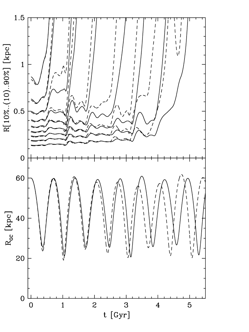
Figure 12:

Figure 13:

Figure 14:

Figure 15:

Figure 16:

Figure 17:

Figure 18:

Figure 19: