Structure and Dynamics of Magnetized Interstellar Clouds: Super-Alfvénic Turbulence?

Abstract

This review summarizes the argument for molecular clouds being dominated by turbulence, most likely super-Alfvénic turbulence. Five lines of observational evidence are given: molecular linewidths and line shapes, nonequilibrium chemical abundances, fractal cloud shapes, measurements of the dispersion of dust extinction through clouds, and Zeeman measurements of the field strength. Recent models by Padoan & Nordlund are summarized, that show that super-Alfvénic turbulence appears consistent with these observations. I then present recent computations of my own, with numerical resolution as high as $256^{3}$ zones, confirming the basic picture proposed by Padoan & Nordlund, but showing that the decay timescales they quote are actually too long. My computations show that decaying turbulence loses its kinetic energy with a $\sim 1/t$ dependence on time regardless of whether the turbulence is subsonic, supersonic, isothermal, adiabatic, unmagnetized or magnetized. Finally, the implications for star formation and turbulence theory are discussed.

Max-Planck-Institut für Astronomie, Königstuhl 17, D-69117 Heidelberg, Germany

1. Introduction

Astronomers have understood qualitatively for at least half a century that the interstellar gas may be in a turbulent state (e. g.  von Weizsäcker 1951). Coming to grips with this understanding in quantitative models nonetheless remains an unfinished task, though not for lack of attempts. Rather, until very recently, most models have had to be, perforce, fully analytic, without guidance from either laboratory or numerical work. Interstellar gas is magnetized, strongly compressible, low viscosity, and has rms velocities far higher than its thermal sound speed. Achieving these conditions in terrestrial laboratories would require extreme measures: even fusion reactors are so small that kinetic instabilities dominate the dynamics. Three-dimensional numerical models with anything approaching adequate resolution have only become possible in this decade: the first transsonic, hydrodynamical model with 256³ grid points, still neglecting magnetic fields, was published by Porter, Pouquet, & Woodward in 1992, and no magnetohydrodynamic (MHD) model with this resolution has yet appeared in the refereed literature, although I will present some preliminary results from such models in this paper, that I hope to have submitted before this paper is published.

The best observed regions of interstellar gas are molecular clouds such as the Orion Molecular Cloud, as their high density allows the formation of CO and other emitting species that can be followed in great detail in mm-wave observations. Molecular clouds appear distinctly clumpy in both position and velocity space, leading to many attempts to characterize them in terms of discrete clumps in a uniform background medium, a viewpoint that can lead to misleading results, as I will show below. The temperatures inferred from line ratios suggest that the observed line widths reflect motions far faster than the local sound speed. Whether these hypersonic velocities produce shocks or not depends on the strength of the magnetic field, which has only been determined in a very small number of regions in molecular clouds, and so remains quite uncertain. A preprint by Padoan & Nordlund (1997; hereafter PN) that I will discuss in this paper puts forward a persuasive argument for the turbulence actually being super-Alfvénic as well as supersonic.

The lifetimes of molecular clouds have been inferred to be several $\times 10^{7}$ yr from the total fraction of gas mass in the Galaxy in the form of molecular gas, and from the lifetimes of the young stars associated with them (Blitz & Shu 1980). The argument has been made that shock formation due to the observed hypersonic velocities would dissipate the energy of the clouds so quickly that the entire clouds would collapse and form stars in a time not much longer than their free-fall times,

$$t_{ff}=(1.4\times 10^{6}\mbox{ yr})(2n(\mbox{H}_{2})/10^{3}\mbox{ cm}^{-3})^{-1/2},$$ (1)

where $n(\mbox{H}_{2})$ is the number density of molecular hydrogen (Goldreich & Kwan 1974, Field 1978).

Three approaches have been taken to try to solve this problem. One, first taken by Arons & Max (1975), is to argue that strong enough magnetic fields will prevent shocks from occurring, and so lengthen the dissipation time. The second, taken by, for example, Scalo & Pumphrey (1982) is to argue, on the basis of clump models, that hydrodynamic turbulence will actually dissipate more slowly than expected. Finally, at Schloß Ringberg, I presented results from PN that showed that MHD turbulence decays nearly as fast as hydrodynamical turbulence. Since then I have done models confirming that result in principle, but showing that all sorts of turbulence appear to decay even faster than they reported, with a time dependence proportional to $\sim 1/t$. If turbulence supports molecular clouds against star formation, it must be constantly driven, by stellar outflows (e. g. Silk & Norman 1980), photoionization (McKee 1989, Bertoldi & McKee 1996), galactic shear (Fleck 1981), or some combination of these or other sources.

2. Review of Molecular Cloud Models

Broadly speaking, four different descriptions of molecular cloud structure have been proposed. The first, and most straightforward, is that the clouds consist of discrete clumps travelling on ballistic orbits under the influence of gravity, colliding occasionally with other clumps. A second description, really a more sophisticated version of the first, has the density distributed in a fractal distribution, but still focusses on self-gravity as the dominant force. The third description invokes subsonic or sub-Alfvénic turbulence, while finally, recent models have invoked supersonic, super-Alfvénic turbulence.

The simplest models of clumpy, turbulent clouds describe the clouds as made up of a large number of spherical gas fragments moving through a lower-density surrounding medium (Scalo & Pumphrey 1982), possibly threaded by a magnetic field (Elmegreen 1985). Scalo & Pumphrey showed that if all collisions were completely inelastic, with any two fragments that came into contact sticking and dissipating their relative energy, the energy would be dissipated on order of a dynamical time $t_{D}=R/\langle v\rangle$, where R is a typical cloud size and $\langle v\rangle$ is the root mean square velocity in the cloud. If the turbulent velocities are fast enough to support the cloud against gravitational collapse, then the resulting estimated dynamical time is just of order the free-fall time $t_{ff}$ (Field 1978). It appears now that this is, in fact, a reasonable estimate of how fast turbulent energy will be dissipated.

However, the picture of turbulence consisting of isolated spherical clumps, when taken literally, has led to worse estimates of the dissipation time scale. For example, Scalo & Pumphrey (1982) then tried to extend their model by taking the geometry of the cloud collisions into account, noting that off-center collisions of spherical clouds would tend not to dissipate all of their energy. The outer parts of each cloud would simply slide by without being strongly influenced by the impact. This reduced the energy dissipation in their model by an order of magnitude, bringing it into rough agreement with cloud lifetimes, but not with more detailed models of turbulence as I discuss below. Elmegreen (1985) included magnetic fields in an otherwise similar model, again reaching the conclusion that dissipation could be much reduced, again in disagreement with more realistic models of magnetized turbulence. The fundamental flaw of such models appears to be the neglect of the space-filling character of even supersonic turbulence, which leads to rapid dissipation of the turbulent energy.

This space-filling character can be described as a fractal structure. Subsonic, incompressible turbulence is measured to have fractal dimension $D=2.3$ (Sreenivasan 1991, also see Sreenivasan & Antonia 1997). That is, measuring the volume of some tracer at different resolutions, the measured volume changes as the resolution changes, as if the tracer occupied a space of dimension intermediate between 2 and 3. It remains unclear whether supersonic, magnetized turbulence has the same fractal dimension, or indeed whether it has constant fractal dimension at all (Chappell & Scalo 1997). Certainly cloud catalogs have been used to derive a fractal dimension $D\sim 2.3$ (Elmegreen & Falgarone 1994). An analytic model of an isothermal molecular cloud that includes just the fractal density distribution and self-gravity has been presented by Pfenniger & Combes (1994), while numerical models are presented by Klessen, Burkert, & Bodenheimer (or some permutation thereof) in these proceedings.

Strong magnetic fields are certainly observed in masers in the densest regions of molecular clouds, and simple flux-conservation arguments suggest that the interstellar field of 3–5 $\mu G$ should be compressed to tens of $\mu G$ in large regions of molecular clouds. Arons & Max (1975) first suggested that MHD waves might drive the observed supersonic motions. Zweibel & Josafatsson (1983) computed the decay rates of such waves and found, in fact, that they decayed within a free-fall time. McKee & Zweibel (1995) and Zweibel & McKee (1995) have shown that as long as such MHD waves are strong, they can support clouds against gravitational collapse. They make the additional prediction that, in that case, the magnetic fields should be in equipartition with the kinetic energy of the gas motions. Gammie & Ostriker (1996) have done 1D numerical models of MHD wave support and dissipation. They find relatively slow dissipation rates for the waves, but our 3D models discussed below suggest that this is due to their imposed symmetry. We have reproduced their results in 1D, but find that in 1D, travelling shocks tend to combine, reducing the dissipation rate, while in 3D, oblique collisions constantly produce vorticity and new shocks.

Attempts to directly detect fields in molecular clouds using OH Zeeman measurements have met with surprisingly limited success, however (Troland et al. 1996), suggesting that magnetic fields may not be as strong as expected. Furthermore, the observed clumpy, possibly fractal, density structure of the clouds is hard to produce with MHD waves. They will only be important if the magnetic energy density exceeds the kinetic energy density. However, in that case, the field will adopt a simple geometry, tending to unfold any tangles or kinks in the field lines. Density enhancements will tend to form sheets perpendicular to the field lines, but not isolated clumps (PN). This leads to the suggestion that super-Alfvénic motions may dominate the structure of molecular clouds, producing structure fairly similar to that seen in simulations of supersonic, unmagnetized turbulence.

3. Observational Evidence

There are at least five lines of observational evidence that support the description of molecular clouds being at least turbulent, and probably supersonically turbulent. The most important is, of course, the dynamical information gleaned from observations of tracer molecules, especially isotopes of CO chosen to be optically thin in the regions observed. Second, examination of the chemistry required to produce the observed abundances of molecules suggests that the individual clumps are out of chemical equilibrium, and must therefore be relatively young. Third, the boundaries of clouds observed in the infrared or in CO emission have fractal properties similar to those of incompressible turbulent flows. Fourth, recent measurements of the dispersion of dust extinction through dark clouds can be naturally reproduced by supersonic turbulent models. Finally, Zeeman measurements of magnetic fields yield values low enough that the observed linewidths correspond to super-Alfvénic motions.

The first clue to the dynamics of molecular clouds is of course the supersonic widths observed in CO lines. I will not attempt to give a full review of these observations, but merely mention two of the major results that are directly relevant. First, Larson (1981) described correlations between linewidth, size, and density of clouds that have guided much subsequent research. Taken at face value, these relations lead to the conclusion that the effective equation of state for the gas in molecular clouds is logotropic (Lizano & Shu 1989), a result that does not agree with turbulent models of the molecular cloud gas (Vázquez-Semadeni, Cantó, & Lizano 1997). However, this may reflect the limited validity of Larson’s Laws, rather than the state of the gas (see, for example, Scalo [1990] or Vázquez-Semadeni, Ballesteros-Paredes, & Rodríguez [1997]). Second, the non-Gaussian shapes of the observed lines have been used to compare models of turbulence with the observations (Falgarone & Phillips 1990). Turbulence is thought to produce intermittency that in turn will produce such non-Gaussian lineshapes, specifically with more power in the wings of the lines than would be expected in a Gaussian.

It has been known for some time that attempts to model the equilibrium chemistry of molecular cloud cores yielded the puzzling result that the early time ($10^{5}$–$10^{6}$ yr) nonequilibrium results appeared more consistent with the observations than the final equilibrium state. A first attempt to understand this was made by Prasad, Heere, & Tarafdar (1991), who used a simple model of core collapse with varying field strengths to follow the combined evolution of the chemistry and the dynamics. Xie, Allen, & Langer (1995) used a mixing-length description of diffusion to try to model chemistry in a turbulent cloud, finding a better match to observations when significant turbulence was included. Bergin et al. (1997) use observations of three cloud cores to come to conclusions similar to Prasad et al. (1991): that the observed chemistry can only be explained by cores with ages of order $10^{5}$ yr. Such young cores are a natural consequence of a turbulent flow in the presence of a background radiation field that keeps low density material in a state typical of the diffuse ISM. Then the only material that will begin to evolve to high-density, shielded, equilibrium states is material that has been swept up in short-lived, turbulent clumps.

Attempts to describe the shapes of molecular clouds at different scales led to the discovery that their boundaries in total column density behave as fractals with a fractal dimension of $D\sim$ 1.3–1.4 (Beech 1987, Dickman, Margulis, & Horvath 1990). Careful examination of the edges of molecular clouds taking into account their velocity structure using high-resolution CO observations by Falgarone, Phillips, & Walker (1991) confirmed this result. Sreenivasan (1991) presents an extensive review of results from terrestrial observations of incompressible hydrodynamical turbulence that shows this dimension to be typical of two-dimensional slices through turbulence. While these results are very suggestive, the relationship between incompressible turbulence and the compressible, magnetized turbulence presumably characteristic of molecular clouds remains uncertain, as does the relationship between two-dimensional slices, and projections of the full three-dimensional distribution into a position-velocity cube.

Background stars can be observed in the near infrared through regions with optical extinction as high as 30 magnitudes. By observing the infrared colors of these stars, their dust reddening can be measured, and so the column density along the line of sight to the star can be derived. Lada et al. (1994) developed this method and applied it to the dark cloud IC 5146. They binned the region into boxes of size 1.5’ in order to measure the mean extinction, and found the very interesting correlation shown in Figure 1: the dispersion in the

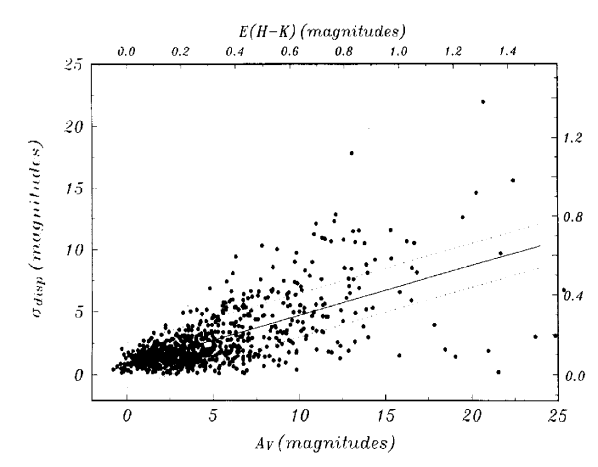
Figure 1.: Comparison of $\sigma_{disp}$, the dispersion in extinction measure across each box, with $A_{V}$, the mean extinction in each box, for the dark cloud IC 5146 (Lada et al. 1994). Also plotted is the linear, least-squares fit to the data.

extinction increases roughly linearly with the mean value. They showed that simple models of cloud structure such as uniform density within each box or isolated clumps drastically failed to reproduce this observation, as shown in Figure 2, but that they could reproduce the observations with

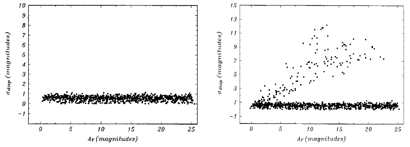
Figure 2.: Two simple models of dispersion in extinction versus mean extinction from Lada et al. (1994). In the left model, extinction varies from box to box, but is uniform in each box, while in the right model foreground stars are added to the stellar population used as sample points.

a power-law variation of column density across each box. Although this column density distribution is quite artificial, a log-normal probability distribution function of density, possibly characteristic of isothermal, supersonic turbulence, has also been shown to reproduce the observed correlation by Padoan, Jones, & Nordlund (1997b), while PN have used direct numerical simulation to reproduce the observation with a weak-field MHD computation, as I will discuss below.

Measurements of the Zeeman effect in OH emission lines from molecular clouds by Crutcher et al. (1993) and Troland et al. (1996) reveal surprisingly low average field strengths $|\vec{B}|_{\parallel}\leq 10\mu$G. If the fields were in equipartition with the kinetic energy, however, the field strengths should be of order 100 $\mu$G (Troland et al. 1996). Several different explanations are suggested by Troland et al., including the possibility that the clouds really are in the state of super-Alfvénic turbulence that a naive interpretation of the results would suggest. They point out however, that unfavorable geometries, tangled fields, or OH abundance changes at high densities could account for the limited observations to date.

4. Models of Supersonic Turbulence

Full hydrodynamical models of molecular clouds were first performed in 2D by Passot, Pouquet & Woodward (1988), showing that even transsonic flows developed the filamentary density enhancements characteristic of molecular clouds. They progressed to 3D in Falgarone et al. (1994), where they simulated observations of the $512^{3}$, transsonic, adiabatic, decaying turbulence simulations of Porter, Pouquet, & Woodward (1994). Models of strongly supersonic, driven turbulence with an isothermal equation of state are briefly referred to in Padoan, Nordlund, & Jones (1997d), although full description is there deferred to a paper still in preparation by Nordlund & Padoan, so it remains unclear how the additional physics actually improves the fit to the observations.

The most important new piece of physics, though, is the inclusion of magnetic fields. Stone (1995; also see Ostriker 1997) and Balsara, Crutcher, & Pouquet (1997) have published preliminary results from 3D models, while Gammie & Ostriker (1996) thoroughly modelled a turbulent, strongly magnetized, molecular cloud in 1D. PN have made a major advance in the field by performing 3D MHD simulations of turbulence in both strongly magnetized and weakly magnetized clouds.

PN used an Eulerian MHD code to model decaying, isothermal turbulence in a box with periodic boundary conditions at a numerical resolution of $128^{3}$ grid points. Their code uses a staggered grid; is fifth order in space and third order in time; uses hyper-diffusive fluxes; and resolves shocks with an artificial viscosity and current sheets with an artifical resistivity. Although the high order of the code is an advantage for smooth flows, eliminating diffusivity except at scales very close to the grid scale, the advantage is lost in flows with shocks or other discontinuities. The discontinuities are resolved over several zones by the artificial viscosity or resistivity just as they would be in a lower-order code; meanwhile the higher order method greatly increases the complexity and computational cost of the code. I present below preliminary models done with ZEUS-3D, which is only second order in space and first order in time, but that use $256^{3}$ zones, or eight times the number of zones of the PN results.

Nevertheless, the interpretation of the two runs presented in PN forces the serious consideration of their suggestion that the turbulent motions in molecular clouds are actually strongly super-Alfvénic. The two runs are started with a solenoidal perturbation of the velocity with root-mean-square (rms) amplitude of Mach 5 and maximum wavenumber of two—that is, the initial perturbations are large and smooth, rather unlike the final turbulent state that has perturbations at all scales. The justification for this is that they believe the driving forces to be from galactic shear, and so coming from large scales initially (Nordlund, private comm., 1997). Self-gravity and ambipolar diffusion are neglected. The field begins uniform and vertical.

The strong field run has initial Alfvén number $A=\langle v\rangle/v_{A}=1$. The initial velocity perturbations were set purely perpendicular to the magnetic field to simulate an initial distribution of Alfvén waves. Although at the end Alfvén waves remain the strongest component, motions parallel to the field have increased to about half the velocity of the perpendicular motions. Advection perpendicular to the field is strongly suppressed, resulting in the formation of sheet-like high-density regions perpendicular to the field. The field remains close to uniform throughout the run, as it is strong enough to resist tangling, as would be true for any field in equipartition with the gas motions.

The weak field run has initial rms Alfvén number $A=10$, with uniform velocity perturbations. Now the gas motions are strong enough to overwhelm the field and it is swept along as the gas forms into the clumps and filaments typical of supersonic hydrodynamic turbulence. The field does dominate initially in the densest swept-up regions, but even in them, advection along field lines can increase the mass-to-flux ratioes significantly over time. Field strengths and directions vary greatly across the region, and the typical morphology is more filamentary or clumpy than sheet-like.

These clear differences between the weak and strong field runs can be compared to the observations. The weak field run reproduces the observations better than the strong field run in at least three ways. First, the clumpy morphology matches the morphology observed in, for example, CO maps. Second, the clumpiness produces column density dispersions that match the Lada et al. (1994) results better than the relatively uniform sheets of the strong-field run, as shown in Figure 3.

Figure 3.: Comparison between dispersion of extinction values and mean extinction values in regions across the numerical models presented by PN. Experiment A is the weak field model, which reproduces the observations shown in Figure 1 significantly better than Experiment B, the strong field model. The values of the extinction were measured at random locations siumulating the random position of a star behind the cloud.

Third, the variation in magnetic field strength with density in the weak field run is better able to reproduce the observed correspondence of magnetic field with density than the strong field run, in which the field remains uniform regardless of the density, as shown in Figure 4. This comes from the model very naturally, because

Figure 4.: Magnetic field strength versus density after one dynamical time in the weak (left) and strong (right) field numerical models of PN, showing that the weak field model reproduces the observed variation of field with density, while the strong field model has the same field strength regardless of local density everywhere. The magnetic field is expressed in units such that $\vec{B}=1$ implies $v_{A}=1$ and $c_{s}=1$ for the mean density $\langle n\rangle$. The bars show the $1\sigma$ dispersion of values in each density bin.

in the strong field case, the field is strong enough to resist compression, and so maintains a roughly uniform strength everywhere, while in the weak field case, the field is carried with the flow, increasing in strength in the same regions the density increases.

Since the meeting, Padoan and his collaborators have submitted papers in which they begin to directly compare their observations with observations in molecular lines. Padoan et al. (1997a) describes a non-LTE radiative transfer computation that they apply to the results of the PN computations to generate simulated observed spectra. They note that the resulting spectra and maps resemble the observations in: morphology; intermittency in the wings of the spectra; smooth central peaks in the integrated lines; multiple components along individual lines of sight; statistical moment distributions; and the linewidth-intensity relation. Padoan et al. (1997c) make comparisons between these simulated observations and actual observations of the Perseus Molecular Cloud, drawing similar conclusions.

I have now reproduced and extended the PN computations myself, using ZEUS (Stone & Norman 1992a, b), and find the same morphology, as described above. However, I find that their decay timescales are strongly dependent on their very smooth initial conditions. Fully developed supersonic turbulence actually appears to decay significantly faster than they claim, whether or not it is dominated by magnetic fields. The problem is that most of the time covered by the computations reported in their paper is taken up by the transition from their smooth initial condition to a turbulent state, so that the actual behavior of the turbulence is only seen at the very end of their runs. In Figure 5 I compare the density distribution shortly after start for a run with maximum wavenumber two, as used by PN, and a run with maximum wavenumber eight. Eventually both runs reach equivalent states, but the run with low wavenumber takes several dynamical times to do so; this initial transient should not be taken as representative of turbulent behavior. We do agree with their ultimate conclusion that the inclusion of magnetic fields does not greatly change the decay timescale of the turbulence, as shown in the right panel of Figure 6, but disagree on what that timescale is.

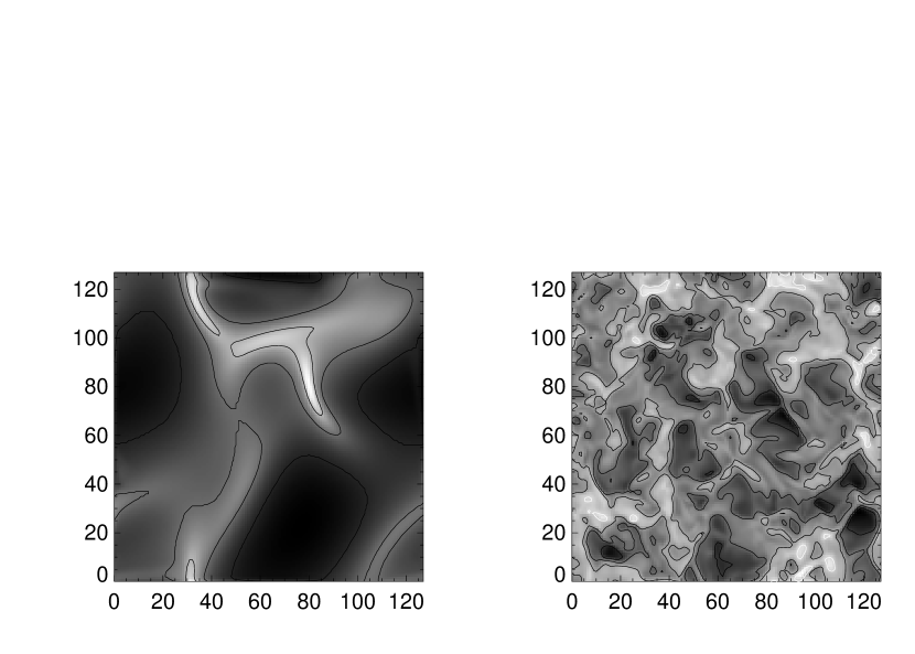
Figure 5.: Comparison of log density for slices through Mach 5 decaying turbulence started with different initial conditions, at a time of $10^{-2}L/c_{s}$, where $L$ is the box size and $c_{s}$ the sound speed. Initial conditions included only wavenumbers up to two on the left, while the initial conditions on the right included wavenumbers up to eight, demonstrating the long transition period required for a low-wavenumber initial condition to reach a fully turbulent state. These computations were performed on a $128^{3}$ grid using ZEUS-3D. The same greyscale is used for both images, covering two orders of magnitude in density.

Our computations have, rather surprisingly, revealed this timescale to be quite universal: undriven turbulence decays as $t^{-\alpha}$, with $\alpha$ in the range $1<\alpha<1.4$, whether the turbulence is subsonic, supersonic, hydrodynamic, magnetically dominated, isothermal or adiabatic, as demonstarted in Figure 6. This result is very well converged as demonstrated in the isothermal, hydrodynamical case in the left panel of this Figure.

Figure 6.: (left) Resolution study for decaying, supersonic, isothermal, hydrodynamic turbulence with initial rms Mach number 5, and numerical resolutions of $32^{3}$ (dotted), $64^{3}$ (short dashed), $128^{3}$ (long dashed), and $256^{3}$ (solid) zones. Time is given in units with $L/c_{s}=20$, where $L=2.0$ is the size of the box and $c_{s}=0.1$ is the sound speed. The initial conditions included perturbations up to a maximum wavenumber of eight. (right) Comparison of decay of kinetic energy for models with different physics at a resolution of $256^{3}$ zones and the same parameters as above: (solid) isothermal hydrodynamics, (dotted) adiabatic hydrodynamics, with adiabatic index $\gamma=1.4$, (short dashed) weakly magnetized, with initial rms Alfvén number $A=5$, (dot-dashed) moderately magnetized, with $A=1$, and (long dashed) strongly magnetized, with $A=0.05$. All lose kinetic energy proportional to $t^{-1}$, similar to the well-resolved hydrodynamic model.

This result is also consistent with experimental measurements (Comte-Bellot & Corrsin 1966, Warhaft & Lumley 1978) and theoretical models (Lesieur 1997) of incompressible turbulence. It is nevertheless quite unexpected, since those theoretical models relied heavily on the specific properties of incompressible hydrodynamic turbulence, rather than universal properties extending across all the types of turbulence we have now simulated.

5. Implications

5.1. Star Formation

If molecular clouds are in a state of driven, super-Alfvénic turbulence, I would outline a scenario for star formation that addresses a number of questions that remained unanswered in the standard scenario of star-formation primarily mediated by ambipolar diffusion in quasi-static cores (e. g.  Mouschovias 1991). One of the reasons that the standard scenario was proposed was to solve the problem of explaining why molecular clouds did not collapse into stars within a single free-fall time.

Under the new scenario, the clouds are supported against collapse by turbulence driven either from galactic shear or local stellar energy sources. Periodically the violent density fluctuations produced by super-Alfvénic shocks will form clumps greater than the local Jeans mass, which will then begin to gravitationally collapse until they are supported by their magnetic fields. If the gravitational binding of these clumps is sufficiently strong, they will no longer be influenced by the surrounding turbulent flow, and can thereafter evolve as described by the standard scenario, producing low mass stars.

Rarely, however, the turbulent converging flows will also produce density concentrations much larger than a local Jeans mass that are immediately magnetically supercritical. Accretion down field lines driven by the external velocity field can raise the central mass-to-flux ratioes of these clumps high enough to collapse without going through a quasi-static phase. This would produce at least intermediate mass stars and perhaps even high mass stars, although there the question of how the countervailing radiation pressure is overcome remains open.

Because they form in a turbulent medium, a wide range of rotational velocities would be expected for both small and large cores. This would lead to a wide range of fragmentation behavior (e. g.  Burkert & Bodenheimer 1996), and a stellar initial mass function that can not be simply derived from from the observed core or clump initial mass function. I note that the attempt by Padoan et al. (1997d) to derive an initial mass function (IMF) from the probability density function of density in supersonic turbulence has been strongly criticized for this and other reasons by Scalo et al. (1997). My personal suspicion is that Adams & Fatuzzo (1996) must come closer to the truth in trying to describe the initial mass function as the result of many random variables operating together. The turbulent production of the parent cores might provide much or all of the necessary randomization. However, they, too, end up with a log-normal IMF that does not necessarily agree well with the observations (Scalo et al. 1997). Sreenivasan (1991, p. 592) points out that the failing assumption here is that all the processes will be distributed so that the central-limit theorem holds, and that turbulent intermittance produces rare but large events that do not follow that theorem. He suggests that a multifractal formalism might provide a way forward, as has now begun to be explored by Chappell & Scalo (1997).

5.2. Turbulence

Our new computations, presented in Figures 6, showing that undriven turbulence decays as approximately $1/t$, emphasize that such turbulence will lose its kinetic energy quickly, regardless of the details of the state of the gas. As the gas in molecular clouds is observed to have significant kinetic energy, that kinetic energy must be supplied from somewhere on a more or less continuous basis. If turbulence supports molecular clouds against star formation, it must be constantly driven, by stellar outflows (e. g. Silk & Norman 1980), photoionization (McKee 1989, Bertoldi & McKee 1996), galactic shear (Fleck 1981), or some combination of these or other sources.

Our computations also suggest that significant progress must be possible in the theory of turbulence, as we have uncovered a general behavior that does not depend on the details of the cascade of energy down to the dissipative scale. Our results must, of course, be compared to experiment, and verified with more sophisticated numerical models—our models do not, for example, include an explicit model for diffusivity, but merely rely on numerical diffusivity to diffuse energy at the smallest scales. The excellent convergence shown in the first panel of Figure 6 suggests, however, that as is usually assumed in classical incompressible turbulence theory, the details of the dissipative process matter rather less than its presence only at the smallest scales.

Acknowledgments.

Original work presented in this paper was done in collaboration with R. Klessen, A. Burkert, and M. D. Smith. Computations were performed at the Rechenzentrum Garching of the Max-Planck-Gesellschaft. I thank E. Vazquez-Semadeni for interesting discussions of turbulence, and P. Padoan for generously allowing the use of figures from his work prior to publication. In preparation of this review I have made extensive use of NASA’s Astrophysics Data System Abstract Service.

References

Adams, F. C., & Fatuzzo, M. 1996, ApJ, 464, 256

Arons, J., & Max, C. E. 1975, ApJ, 196, L77

Balsara, D. S., Crutcher, R. M., & Pouquet, A. 1997, in Star Formation Near and Far, eds. S. S. Holt & L. G. Mundy (Woodbury, NY: American Institute of Physics Press), 89

Beech, M. 1987, Astroph. Sp. Sci. 133, 193

Bergin, E. A., Goldsmith, P. F., Snell, R. L., & Langer, W. D. 1997, ApJ, 482, 285

Bertoldi, F., & McKee, C. F. 1996, in Amazing Light, ed. R. Y. Chiao (New York: Springer), 41

Blitz, L., & Shu, F. H. 1980, ApJ, 238, 148

Burkert, A., & Bodenheimer, P. 1996, MNRAS, 280, 1190

Chappell, D. W., & Scalo, J. 1997, preprint (astro-ph/9707102)

Comte-Bellot, G. & Corrsin, S. 1966, J. Fluid Mech., 25, 657

Crutcher, R. M., Troland, T. H., Goodman, A. A., Heiles, C., Kazès, I., & Myers, P. C. 1993, ApJ, 407, 175

Dickman, R. L., Margulis, M., & Horvath, M. A. 1990, ApJ, 365, 586

Elmegreen, B. G. 1985, ApJ, 299, 196

Elmegreen, B. G., & Falgarone, E. 1994, ApJ, 471, 816

Falgarone, E., Lis, D. C., Phillips, T. G., Pouquet, A., Porter, D. H., & Woodward, P. R. 1994, ApJ, 436, 728

Falgarone, E., & Phillips, T. G. 1990, ApJ, 359, 344

Falgarone, E., Phillips, T. G., & Walker, C. K. 1991, ApJ, 378, 186

Field, G. B. 1978, in Protostars & Planets, ed. T. Gehrels (Tucson: Univ. of Arizona Press), 243

Fleck, R. C., Jr. 1981, ApJ, 246, L151

Gammie, C. F., & Ostriker, E. C. 1996, ApJ, 466, 814

Goldreich, P., & Kwan, J. 1974, ApJ, 189, 441

Lada, C., Lada, E., Clemens, D. P., & Bally, J. 1994, ApJ, 429, 694

Larson, R. B. 1981, MNRAS, 194, 809

Lesieur, M. 1997, Turbulence in Fluids, 3rd ed. (Dordrecht: Kluwer), 245

Lizano, S., & Shu, F. 1989, ApJ, 342, 834

McKee, C. F. 1989, ApJ, 345, 782

McKee, C. F., & Zweibel, E. G. 1995, ApJ, 440, 686

Mouschovias, T. Ch. 1991, in The Physics of Star Formation and Early Stellar Evolution, eds. C. J. Lada & N. D. Kylafis (Dordrecht: Kluwer), 449

Ostriker, E. 1997 in Star Formation Near and Far, eds. S. S. Holt & L. G. Mundy (Woodbury, NY: American Institute of Physics Press), 51

Padoan, P., Bally, J., Billawala, Y., Juvela, M., & Nordlund, Å. 1997a, ApJ, submitted

Padoan, P., Jones, B. J. T., & Nordlund, Å, 1997b. ApJ, 474, 730

Padoan, P., Juvela, M., Bally, J., & Nordlund, Å. 1997c, ApJ, submitted

Padoan, P., & Nordlund, Å. 1997, ApJ, submitted (astro-ph/970616) (PN)

Padoan, P., Nordlund, Å, & Jones, B. J. T. 1997d, MNRAS, in press (astro-ph/9703110)

Passot, T., Pouquet, A., & Woodward, P. 1988, A&A, 197, 228

Pfenniger, D., & Combes, F. 1994, A&A, 285, 94

Porter, D. H., Pouquet, A, & Woodward, P. R. 1992, Phys. Rev. Lett. 68, 3156

Porter, D. H., Pouquet, A, & Woodward, P. R. 1994, Phys. Fluids, 6, 2133

Prasad, S. S., Heere, K. R., & Tarafdar, S. P. 1991, ApJ, 373, 123

Scalo, J. M. 1990, in Physical Processes in Fragmentation and Star Formation, eds. R. Capuzzo-dolcetta, C. Chiosi, & A. D. Fazio (Dordrecht: Kluwer), 151

Scalo, J. M., & Pumphrey, W. A. 1982, ApJ, 258, L29

Scalo, J., Vázquez-Semadeni, E., Chappell, D., & Passot, T. 1997, ApJ, submitted (astro-ph/9710075)

Silk, J., & Norman, C. 1980, in Interstellar Molecules, IAU Symposium 87, ed. B. H. Andrew (Dordrecht: Reidel), 165

Sreenivasan, K. R. 1991, Ann. Rev. Fluid Mech., 23, 539

Sreenivasan, K. R., & Antonia, R. A. 1997, Ann. Rev. Fluid Mech. 29, 435

Stone, J. M. 1995, in Clouds, Cores, and Low Mass Stars, eds. D. Clemens & R. Barvainis, ASP Conference Series Vol. 65, (Dordrecht: Kluwer)

Stone, J. M., & Norman, M. L. 1992a, ApJS, 80, 753

 . 1992b, ApJS, 80, 791

Troland, T. H., Crutcher, R. M., Goodman, A. A., Heiles, C., Kazès, I., & Myers, P. C. 1996, ApJ, 471, 302

Vázquez-Semadeni, E., Ballesteros-Paredes, J., & Rodríguez, L. F. 1997, ApJ, 474, 292

Vázquez-Semadeni, E., Ballesteros-Paredes, J., & Rodríguez, L. F. 1997, ApJ, 474, 292

Vázquez-Semadeni, E., Cantó, J., & Lizano, S. 1997, ApJ, submitted (astro-ph/9708148)

von Weizsäcker, C. F. 1951, ApJ, 114, 165

Warhaft, Z. & Lumley, J. L. 1978, J. Fluid Mech. 88, 659

Xie, T., Allen, M., & Langer, W. D. 1995, ApJ, 440, 674

Zweibel, E. G., & Josafatsson, K. 1983, ApJ, 270, 511

Zweibel, E. G., & McKee, C. F. 1995, ApJ, 439, 779