Modelling of the nonthermal flares in the galactic

microquasar GRS 1915+105

A. M. Atoyan^1,2 and F. A. Aharonian¹

¹ Max-Planck-Institut für Kernphysik, Postfach 103980, D-69029 Heidelberg, Germany

² Yerevan Physics Institute, Alikhanian Brothers 2, 375036 Yerevan, Armenia

Abstract

The microquasars recently discovered in our Galaxy offer unique opportunity for a deep insight into the physical processes in relativistic jets observed in different source populations. We study the temporal and spectral evolution of the radio flares detected from the relativistic ejecta in the microquasar GRS 1915+105, and propose a model which suggests that these flares are due to synchrotron radiation of relativistic electrons suffering adiabatic and escape losses in fastly expanding plasmoids (the radio clouds). Analytical solutions to the kinetic equation for relativistic electrons in the expanding magnetized clouds are found, and the synchrotron radiation of these electrons is calculated. Detailed comparison of the calculated radio fluxes with the ones detected from the prominent flare of GRS 1915+105 during March/April 1994 provides conclusive information on the basic parameters in the ejecta, such as the absolute values and temporal evolution of the magnetic field, speed of expansion, the rate of continuous injection of relativistic electrons into and their energy-dependent escape from the clouds, etc. The data of radio monitoring of the pair of resolved ejecta enable unambiguous determination of parameters of the bulk motion of counter ejecta and the degree of asymmetry between them, as well as contain important information on the prime energy source for accelerated electrons, in particular, may distinguish between the scenarios of bow shock powered and relativistic magnetized wind powered plasmoids. Assuming that the electrons in the ejecta might be accelerated up to very high energies, we calculate the fluxes of synchrotron radiation up to hard X-rays/soft $\gamma$-rays, and inverse Compton GeV/TeV $\gamma$-rays expected during radio flares, and discuss the implications which could follow from either positive detection or flux upper limits of these energetic photons.

Key words: radiation mechanisms: nonthermal – radio continuum: stars – stars: individual: GRS 1915+105 – gamma-rays: theory – galaxies: jets

e-mails:
A.Atoyan – atoyan@fel.mpi-hd.mpg.de
F.Aharonian – aharon@fel.mpi-hd.mpg.de

1 Introduction

The hard X-ray transient GRS 1915+105 discovered in 1992 (Castro-Tirado et al. 1992) belongs to the class of galactic black hole (BH) candidate sources characterized by an estimated mass of the compact object $M\geq 3M_{\odot}$, strong variability of the electromagnetic radiation, with the spectra extending to energies beyond $100\,\rm keV$ (e.g. see Harmon et al. 1994). The invoking similarity of these sources with AGNs, the objects powered by the accreting BHs of essentially larger mass scales, has recently found a new convincing evidence, after the discovery of apparent superluminal jets in GRS 1915+105 (Mirabel & Rodriguez 1994, hereafter MR94), and in another hard X-ray transient, GRO J1655-40 (Tingay et al. 1995, Hjellming & Rupen 1995). The existence of relativistic jets in these galactic sources, called “microquasars”, makes them unique cosmic laboratories for a deeper insight into the complex phenomenon of the jets common in those powerful extragalactic objects (Mirabel & Rodriguez 1995). Indeed, being much closer to us than AGNs, the microquasars offer an opportunity for monitoring of the jets in a much shorter spatial and temporal scales. Furthermore, the parameter $L_{\rm Edd}/d^{2}$, where t$L_{\rm Edd}\simeq 1.3\times 10^{38}(M/M_{\odot})\,\rm erg/s\,$ is the Eddington luminosity (an indicator of the potential power of the source), and $d$ is the distance to the source, is typically by 2-4 orders of magnitude higher for the galactic BH candidates than for AGNs. This enables detection of the galactic superluminal jets with Doppler factors even as small as $\delta\leq 1$, in contrast to the case of jets in blazars (AGNs with jets close to the line of sight), for detection of which strong Doppler boosting of the radiation, due to $\delta\gg 1$, is generally needed. Importantly, for the jets with aspect angles close to $90^{\circ}$ (which is the case in both GRS 1915+105 and GRO J1655-40), the Doppler factors of the approaching and receding components are comparable, so both these components may be detectable (see Mirabel & Rodriguez 1995).

In this paper we present the results of theoretical study of the nonthermal flares of GRS 1915+105, which are observed in the radio (MR94; Mirabel & Rodriguez 1995; Rodriguez et al. 1995; Foster et al. 1996) and possibly also infra-red (Sams et al. 1996; Fender et al. 1997) bands, and can be expected at higher photon energies as well, if the electrons in the ejecta are accelerated up to very high energies (VHE). The main part of the paper is devoted to the explanation of the radio flares observed, which provide important information about the principal parameters and processes in the radio emitting plasmoids (i.e. the clouds containing relativistic electrons and magnetic fields). In Section 2 we deduce, on the basis of qualitative consideration, the principal scenario for interpretation of these flares. In Section 3 we obtain analytical solutions to the kinetic equation which describes the temporal evolution of relativistic electrons in an expanding magnetized medium. In Section 4 we carry out detailed comparison of the fluxes of synchrotron radiation emerging from the model radio clouds with the temporal and spectral characteristics of the fluxes observed during the prominent March/April 1994 flare of GRS 1915+105 (MR94), which provides conclusive constraints for the model parameters of the ejecta. The data of radio monitoring of the two (approaching and receding) ejecta present particular interest. We show that these data not only enable unambiguous determination of the aspect angle and the speed of propagation of the twin ejecta (which perhaps are a little asymmetrical, as follows from the observed flux ratio of the counter components), but also contain an important information about the prime energy source for continuous energization of the plasmoids.

For any reasonable assumption about the magnetic field in the ejecta, the energy spectrum of relativistic electrons should extend at least up to energies of a few GeV. It is not excluded, however, that the electrons in the ejecta are accelerated beyond these energies. Therefore, after determination of the range of basic parameters of the expanding plasmoids, in Section 5 we speculate that in GRS 1915+105, similar to the case of BL Lacs (e.g. Urry & Padovani 1995; Ghisellini & Maraschi 1997), the electrons may be accelerated beyond TeV energies, $E\geq 10^{12}\,\rm eV$, and discuss the fluxes of synchrotron radiation which could then extend up to X-ray/$\gamma$-ray energies, as well as the fluxes of the inverse Compton (IC) $\gamma$-rays expected in the high and very high energies. In Section 6 we summarize the main results of the paper.

2 Basic estimates

2.1 Radio fluxes during outbursts

Observations of GRS 1915+105 show that the radio emission of the source in its active state is characterized by the increase of the radio emission at $\nu\sim(1-10)\,\rm GHz$ from the flux level $S_{\nu}\leq 10\,\rm mJy$ to $S_{\nu}\sim 100\,\rm mJy$ (the plateau state, according to Foster et al. 1996), on top of which the episodes of radio flares, with durations from days to a month and fluxes up to $\sim 1\,\rm Jy\,$, are superimposed. The spectra in the plateau state are flat or inverted, $\alpha_{\rm r}\leq 0$ (approximating $S_{\nu}\propto\nu^{-\alpha_{\rm r}}$), which is a typical indicative for a strong synchrotron self-absorption in the source (e.g. Pacholczyk 1970). The radio flares, which most probably are related with the events of ejection of radio clouds, are distinguished by very rapid, less than a day, rise of the fluxes by several times, which then decay on timescales of days or more. Remarkably, already at the rising stage of the flares the spectra reveal transition from optically thick ($\alpha_{\rm r}\leq 0$) to optically thin ($\alpha_{\rm r}>0$) emission. Initially, when the fluxes are at the maximum level, the spectra are typically hard, with $\alpha_{\rm r}\sim 0.5$, which may then steepen to $\alpha_{\rm r}\sim 1$.

Convincing examples of such spectral behavior are given by Rodriguez et al (1995) where the detailed data of radio monitoring of GRS 1915+105 at different wavelengths during 5 months from 1 December 1993 to 30 April 1994 are summarized. Thus, from Table 1 of Rodriguez et al. (1995) it is seen that the spectrum of the flare on December 6.0, 1993, measured with VLA radio telescopes simultaneously at 5 different frequencies from $\approx 1.47\,\rm GHz$ to 22.49 GHz was self-absorbed in the range of $1.47\leq\nu\leq 4.89\,\rm GHz$ ($\alpha_{\rm r}\approx-0.73$), whereas at higher frequencies it corresponded to optically thin synchrotron emission, with the mean slope $\alpha_{\rm r}\simeq 0.52$ in the range of $4.89\leq\nu\leq 22.49\,\rm GHz$. On that day the flux at $\nu\approx 4.89\,\rm GHz$ was $S_{\nu}\approx 500\,\rm mJy$ . Meanwhile, on November 29.97 the fluxes were at the level of $\simeq 100\,\rm mJy$, and the spectrum was inverted in the range up to at least $15\,\rm GHz$. By December 6.6 the fluxes have increased further, reaching $S_{\nu}=1083\,\rm mJy$ at 3.28 GHz. Comparison with the flux measured simultaneously by IRAM telescope at $\nu=234\,\rm GHz$ (Rodriguez et al. 1995) shows that in this broad range the spectrum was ‘optically thin’, with $\alpha_{\rm r}=0.51$, indicating that the source during $\leq 14$ hours became transparent at 9 cm band.

An example of gradual steepening of initially hard spectra, with $\alpha_{\rm r}\sim 0.5$ at the stage of flare maximum, is provided by the outburst on 11 December 1993, when the fluxes measured by Nancay telescope at 21 and 9 cm have increased to 1319 and 901 mJy, respectively ($\alpha_{\rm r}\simeq 0.45$). On the next day the fluxes have decreased by factor of 2, while the spectrum steepened to $\alpha_{\rm r}\simeq 0.6\,$. Gradual steepening of the radio spectra in time is obvious also in the multiwavelength VLA data taken on December 14, 16 and 17, when the spectral slope between 4.89 and 22.49 GHz was changing as $\alpha_{\rm r}\simeq 0.72,\,0.83$ and 1.1, respectively (see Rodriguez et al. 1995).

Similar spectral evolution, although on significantly larger timescales, was observed for the prominent strong radio outburst of 19 March 1994, when for the first time a pare of counter ejecta were resolved, and superluminal motion in the Galaxy was discovered (MR94). On March 24 the spectral index at $\lambda\sim 3.5\,\rm cm$ was $\alpha_{\rm r}\simeq 0.5\,$, which by April 16 steepened to $\alpha_{\rm r}\simeq 0.8\,$. For an estimated distance $d=12.5\pm 1.5\,\rm kpc$ to GRS 1915+105 , the apparent velocities of the approaching and receding ejecta made $1.25\pm 0.15$ and $0.65\pm 0.08$ speed of light, respectively, using which the real speed $\beta\simeq 0.92$ of the ejecta moving in the opposite directions at an angle $\theta\simeq 70^{\circ}$ to the line of sight was inferred (MR94).

Importantly, since both radio emitting components of this strong and long-lived flare were resolved, the data of radio monitoring of this flare presented in MR94 contain a unique information about the processes in the jets. Thus, the detection of the receding component enables measurement of the flux ratio $S_{\rm a}/S_{\rm r}$ of the approaching and receding ejecta. In the case of identical jets, the ratio of the flux densities measured at equal angular separations of the jets from the core is

$$\frac{S_{\rm a}}{S_{\rm r}}=\left(\frac{1+\beta\cos\theta}{1-\beta\cos\theta}\right)^{j+\alpha_{\rm r}}\;,$$ (1)

where $j=3$, if the fluxes are produced in the moving discrete radio clouds, but $j=2$ for the brightness ratio of continuous stationary jets (e.g. see Lind & Blandford 1985). The radio patterns of the March-April flare clearly show motion of two discrete components, but not a stationary jet emission. Then, for the deduced values of $\beta\simeq 0.92$ and $\theta=70^{\circ}$, equation (1) predicts the flux ratio $S_{\rm a}/S_{\rm r}\simeq 12$, while $S_{\rm a}/S_{\rm r}=8\pm 1$ is observed (MR94). This discrepancy between the observed and expected flux ratios can be interpreted as an indication of shocks propagating with the speed $\beta\simeq 0.92$ in the continuous fluid of radio emitting plasma which is steaming with a velocity $\beta_{\rm f}\simeq 0.7$ (Bodo & Ghisellini 1995). However, it is possible also to explain (Atoyan & Aharonian 1997) the observed flux ratio in terms of motion of discrete radio sources with the speeds coinciding with the deduced pattern speed, if one would allow for the twin ejecta be similar, but not necessarily identical, as implied in equation (1). In Section 4 we will show that the ‘discrepancy’ between the observed and expected flux ratios are easily removed by a small asymmetry between the intrinsic parameters of the ejecta, e.g. by small difference in the velocities $\beta_{\rm a}$ and $\beta_{\rm r}$ of the approaching and receding clouds. Then, deviations of $S_{\rm a}/S_{\rm r}$ from the ‘expected’ value can be rather considered as a measure of asymmetry between the twin ejecta.

2.2 Radio electrons

Generally, gradual transition from self-absorbed to optically thin spectra at progressively lower frequencies is a typical indicator of the synchrotron radiation of an expanding radio cloud. Power-law radiation spectra with $\alpha_{\rm r}\simeq 0.5$ imply power-law distribution of relativistic electrons $N(\gamma)\propto\gamma^{-\alpha_{\rm e}}$ with the exponent $\alpha_{\rm e}=2\,\alpha_{\rm r}+1\simeq 2$. Since these radio spectra span a broad interval of frequencies from $\sim 1\,\rm GHz$ up to $\leq 250\,\rm GHz$, the electron distribution should be power-law within some interval of energies $\gamma_{1}\leq\gamma\leq\gamma_{2}\,$, with the ratio of Lorentz factors $\gamma_{2}/\gamma_{1}>10$. To estimate the range of basic parameters of radio clouds, such as the magnetic field $B$, size $R$, speed of expansion $v_{\rm exp}$, etc., in this section we will suppose pure power-law electron distribution, $N(\gamma)=A_{0}\gamma^{-2}$, extending from $\gamma_{1}=1$ up to $\gamma_{2}=\gamma_{\rm max}$, with a sharp cut-off above $\gamma_{\rm max}$, i.e. $N(\gamma>\gamma_{\rm max})=0$. For this spectrum of electrons $A_{0}$ actually corresponds to the total number of relativistic electrons, $N_{\rm e}=A_{0}$, and the total energy in the electrons is $W_{\rm e}=A_{0}\,m_{\rm e}c^{2}\ln\gamma_{\rm max}$.

Characteristic frequency of synchrotron photons emitted by an electron with Lorentz factor $\gamma$ in the magnetic field B is $\nu_{\rm s}\simeq 0.3\times(1.5\nu_{\rm\,B}\,\gamma^{2})$, where $\nu_{\rm\,B}=eB\sin\vartheta/2\pi m_{\rm e}c$, and $\vartheta$ is the pitch angle (e.g. Ginzburg 1979). For the mean $\overline{\sin\vartheta}=\sqrt{2/3}$, the frequency

$$\nu_{\rm s}\simeq 10^{6}\,B\gamma^{2}\;\rm Hz\,,$$ (2)

where $B$ is in Gauss. Since the magnetic fields expected in the cloud $B\sim(0.03-0.3)\,\rm G$ (see below), for production of synchrotron photons at $\nu\sim 300\,\rm GHz$, electrons with $\gamma\sim$ few times $10^{3}$ are required. In the case of synchrotron origin of the IR jet observed by Sams et al. (1996), or of the rapid IR flares detected by Fender et al. (1997) in GRS 1915+105, relativistic electrons with $\gamma\gg 10^{4}$ are to be supposed. However, in the first part of this paper, where we study the radio fluxes, we will not speculate with such possibility and will limit the range of relativistic electrons under consideration with $\gamma_{\rm max}=10^{4}$.

2.3 Magnetic fields, size, and speed of expansion of radio clouds

In the case of an isotropic source with luminosity $L^{\prime}(\nu^{\prime})$ in its rest frame, an observer at a distance $d$ would detect the flux $S_{\nu}=\delta^{3}L^{\prime}(\nu/\delta)/4\pi d^{2}$, where $\delta=\sqrt{1-\beta^{2}}/(1-\beta\cos\theta)$ is the Doppler factor of the source moving with a speed $\beta$ at an angle $\theta$ to the line of sight (e.g. Lind & Blandford 1985). For distances $d_{\ast}\equiv d/12.5{\,\rm kpc}\simeq 1$, the fluxes expected from an optically thin cloud are

$$S_{\nu}\simeq 2\times 10^{-39}\,A_{0}\,\delta^{7/2}\,B^{3/2}\,\nu^{-1/2}\,d_{\ast}^{-2}\;\rm mJy\;.$$ (3)

Introducing the ratio $\eta=w_{\rm e}/w_{\rm B}$ of the energy densities of relativistic electrons $w_{\rm e}=3W_{\rm e}/4\pi R^{3}$ to the energy density of the magnetic field $w_{\rm B}=B^{2}/8\pi$ in the cloud, the coefficient $A_{0}$ can be expressed as $A_{0}=2\times 10^{50}\,\eta\,B^{2}R_{15}^{3}$, where $R_{15}$ is the characteristic radius $R$ of the cloud in units of $10^{15}\,\rm cm$. Since the radio fluxes observed at $\nu\sim 10\,\rm GHz$ reach the level $\sim 500\,\rm mJy$ (for strong flares), the magnetic field in the emission region should be

$$B=7.7\times 10^{-2}\,\delta^{-1}\,\eta^{-2/7}R_{15}^{-6/7}d_{\ast}^{4/7}S_{\ast}^{2/7}\;\rm G\;,$$ (4)

where $S_{\ast}\equiv S_{\rm 10\,GHz}/500\,\rm mJy$.

The cloud’s radius $R$ can be estimated from the requirement of optical transparency of the source with respect to synchrotron self absorption. Calculation of the absorption coefficient for the supposed power-law spectrum of electrons is straightforward (e.g. Ginzburg 1979), resulting in $\kappa_{\nu}=4.4\times 10^{15}\eta B^{4}\nu^{-3}\,\rm cm^{-1}$. Using equation (4), the size $R$ of the cloud can be expressed in terms of the opacity $\tau_{\nu}=R\,\kappa_{\nu}$ at a given frequency $\nu$:

$$R_{15}=\,0.46\,\delta^{-28/17}\eta^{-1/17}d_{\ast}^{16/17}S_{\ast}^{8/17}\tau_{\nu}^{-7/17}\nu_{\rm GHz}^{-21/17}\;,$$ (5)

where $\nu_{\rm GHz}\equiv\nu/1\,\rm GHz$. Then from equation (4) follows that

$$B\simeq 0.15\,\delta^{7/17}\eta^{-4/17}d_{\ast}^{-4/17}S_{\ast}^{-2/17}\tau_{\nu}^{6/17}\nu_{\rm GHz}^{18/17}\;\rm G.$$ (6)

For the ejecta in GRS 1915+105 the Doppler factor $\delta\simeq 0.6$ (MR94), so the optical transparency $\tau_{\nu}\leq 1$ at frequencies $\nu\sim(1.4-3)\,\rm GHz$ requires a magnetic field at the stage of flare maximum $B\sim(0.2-0.3)$ Gauss, if the energy densities of relativistic electrons and magnetic fields in the ejecta would be at the equipartition level $\eta\sim 1$.

Due to rather weak dependence of $B$ on the opacity $\tau_{\nu}$, the equipartition magnetic field $B_{\rm eq}$ could be significantly less than $0.2\,\rm Gauss$ only if $\tau_{\nu}\leq 0.1$. However, to reach even $\tau_{\nu}=1$ in a few days after ejection, the clouds should expand with a very high speeds comparable with the speed of light. Indeed, from equation (5) follows that the characteristic size of the clouds ejected on 19.8 March 1994, should increase to $R\simeq 8\times 10^{14}\tau_{1.4\,\rm GHz}^{-0.41}\,\rm cm$ by 24.3 March, $\Delta t\simeq 4.5\,\rm days$ after the ejection event, when the flare was detected by Nancy telescope (Rodriguez et al. 1995). Then, since the intrinsic time in the rest frame of the cloud $\Delta t^{\prime}=\delta\,\Delta t$, a speed of expansion $v_{\rm exp}>0.1\times c$ is to be supposed to provide $\tau_{1.4\,\rm GHz}\leq 1$. Expansion speeds even higher could be needed for the flares which may be weaker, but become transparent during $\Delta t\leq 1\,\rm day$. For example, for the radio flare reported by Gerard (1996), apparent evolution of the fluxes, measured at 9 and 21 cm, from an inverted spectrum to the one with $\alpha_{\rm r}\simeq 0.5$ occurred between 9.0 and 10.0 of July 1996, when the flux at 21 cm has increased from $S_{\rm 1.4\,GHz}<30\,\rm mJy$ to $S_{\rm 1.4\,GHz}=140\,\rm mJy$. Using equation (5), an expansion speed $v_{\rm exp}\geq 0.2\,c$ (!) is found. Thus, transition of the flares from optically thick to thin spectral forms on timescales of days implies that the radio clouds are expanding with velocities $v_{\rm exp}\geq(0.1-0.2)\,c$. This estimate agrees with the clouds expansion speed deduced from the observations, and suggests that the lack of red-shifted optical lines from GRS 1915+105 might be due to their large Doppler broadening (Mirabel et al. 1997).

2.4 Steepening of the radio spectra: implications

The observed gradual steepening of the radio spectra from initial $\alpha_{\rm r}\sim 0.5$ to $\alpha_{\rm r}\sim 1$ at the stage of fading of the flares, requires a steepening of the energy distribution of the parent electrons from the power-law exponent $\alpha_{\rm e}\sim 2$ to $\alpha_{\rm e}\sim 3$. The steepening of the electron spectral index by factor of 1 is usually attributed to the synchrotron (or inverse Compton) energy losses of the electrons, $P_{\rm s}(\gamma)\propto\gamma^{2}$, and for extragalactic jets the models of this kind were considered in a number of papers (e.g., Marscher 1980; Königl 1981; Bloom & Marscher 1996; etc). In the case of GRS 1915+105, however, such an interpretation of the radio data is impossible. Indeed, the synchrotron energy loss time of an electron with energy $\gamma$ is

$$t_{\rm s}(\gamma)\simeq 7.7\times 10^{8}\,\gamma^{-1}B^{-2}\;\rm s.$$ (7)

Using equation (2), the time needed for modification of the electron spectra, in the range of energies responsible for the synchrotron radiation at frequencies $\nu$, is found:

$$t_{\rm s}(\nu)\simeq 2.4\times 10^{7}\,\nu_{\rm GHz}^{-1/2}B^{-3/2}\;\rm s.$$ (8)

Thus, in the magnetic fields limited by equation (6), the synchrotron losses of the electrons cannot be responsible for the steepening of the radio spectra, since even for frequencies $\nu\sim 10\,\rm GHz$ they would require timescales larger than few years.

There are two principle possibilities to explain the observed spectral evolution. The first one is to assume that the relativistic electrons are continuously injected into the cloud with a spectrum $Q(\gamma,t)\propto\gamma^{-\alpha_{\rm inj}}$, with the power-law index $\alpha_{\rm inj}=2$ during the first $(1-3)$ days, which later on steepens to $\alpha_{\rm inj}\geq 3$ so as to provide the steepening of the prompt distribution of electrons $N(\gamma,t)$ to the power-law index $\alpha_{\rm e}\sim 3$. The second option is to assume energy-dependent escape of electrons from the cloud, while the injection spectrum would not necessarily steepen. Note that in this case as well one needs a continuous injection of the electrons, since otherwise for any escape-time $\tau_{\rm esc}(\gamma)$ the escape of electrons would result in a distribution $N(\gamma,t)$ with a sharp (exponential) cut-off, instead of power-law modification, above some $\gamma^{\prime}$ defined from the equation $\tau_{\rm esc}(\gamma^{\prime})=t$ (see Section 3). Thus, in both cases a proper interpretation of the spectral steepening during the flare implies continuous injection of relativistic electrons into the clouds.

In principle, neither of those two options can be excluded without specification of $Q(\gamma,t)$ and detailed calculation of the electron distribution $N(\gamma,t)$. However, there are some arguments in favor of the escape of relativistic electrons as the main reason for the steepening of radio spectra. Indeed, let us suppose that the electron escape is negligible. Then, in order to modify the electron distribution from the power-law index $\alpha_{\rm e}\sim 2$ at $t_{1}\simeq(1-3)\,\rm days$ to $\alpha_{\rm e}\rightarrow 3$ at $t\sim 2\,t_{1}$ (as observed), the injection of electrons with the steep spectrum $\alpha_{\rm inj}\geq 3$ should proceed at least with the same rate $Q(\gamma,t)$ as initially. However, contrary to this requirement, strong steepening of the injection spectrum generally indicates that the efficiency of particle acceleration is essentially suppressed, so significant decline of the injection rate $Q(\gamma,t)$ would have to be expected. Meanwhile, assuming fast escape of relativistic electrons from the cloud, the old ‘hard spectrum’ electrons could be replaced with a freshly injected ‘soft’ ones on timescales $\sim\tau_{\rm esc}$. Moreover, since $N(\gamma,t)\sim Q(\gamma,t)\,\tau_{\rm esc}$ (for $t\gg\tau_{\rm esc}$), then an energy-dependent escape, $\tau_{\rm esc}(\gamma)\propto\gamma^{\Delta}$ with $\Delta\leq 1$, could provide the required steepening of $N(\gamma,t)$ even for the same hard injection spectrum $Q\propto\gamma^{-2}$ as initially. This is an important possibility, since as we shall see later, the decline of $S_{\nu}(t)$ observed during March-April 1994 (MR94) implies substantial injection of relativistic electrons into the radio clouds at all stages of the flare evolution.

2.5 Energetics

The energy $W_{\rm B}$ of the magnetic field in the radio cloud can be estimated using equation (4):

$$W_{\rm B}\simeq 9.9\times 10^{41}\,\delta^{-2}\eta^{-4/7}R_{15}^{9/7}d_{\ast}^{8/7}S_{\ast}^{4/7}\;{\rm erg}\,.$$ (9)

The energy of relativistic electrons $W_{\rm e}=\eta W_{\rm B}$, therefore the total energy $W_{\rm tot}=W_{\rm e}+W_{\rm B}\propto(\eta^{3/7}+\eta^{-4/7})$ reaches the minimum at $\eta=4/3$, i.e. around equipartition between magnetic field and relativistic electrons in the cloud (e.g. Pacholczyk 1970). For the ejecta in GRS 1915+105 with $\delta\simeq 0.6$, the minimum energy in radio electrons at the stage of flare maximum can be estimated as $W_{\rm e}\sim 3\times 10^{42}\,\rm erg$, which requires continuous injection of the electrons with the mean power $P_{\rm inj}\simeq(1-3)\times 10^{37}\,\rm erg/s$ during $\Delta t^{\prime}\sim 1-3\,\rm days$. This estimate is in agreement with the one obtained by Liang & Li (1995), however, it does not take into account the adiabatic energy losses of electrons in the rapidly expanding cloud. As it is shown by accurate numerical calculations in Section 4, the adiabatic losses result in an increase of the electron injection needed to the level of $P_{\rm inj}\sim 10^{38}\,\rm erg/s$. Note that the power needed for bulk acceleration of the ejecta in GRS 1915+105 is estimated as $P_{\rm jet}\sim(1-5)\times 10^{38}\,\rm erg/s$ (Meier 1996).

The value of $P_{\rm inj}\sim 10^{38}\,\rm erg/s$ corresponds to the minimum power of relativistic electrons to be injected into the cloud. In the case of deviation of the magnetic field $B$ in the cloud from its ‘equipartition’ value $B_{\rm eq}$, the energy requirements would be significantly higher. Defining $B_{\rm eq}$ as a magnetic field for which $\eta=1$, from equation (6) follows that $\eta=(B/B_{\rm eq})^{-17/4}$. It means that a decrease of $B$ by an order of magnitude is to be compensated by an increase of $\eta$ by four orders of magnitude, and correspondingly the increase of $W_{\rm e}\propto\eta^{3/7}$ by almost 2 orders of magnitude, to provide the same flux $S_{\ast}$. Thus, assuming a magnetic field $B_{0}\sim 0.03\,\rm G$ at times $t\sim 3\,\rm days$ after ejection (when the cloud’s radius $R\sim 10^{15}\,\rm cm$), instead of $B_{\rm eq}\simeq(0.2-0.3)\,\rm G$, one has to suppose $P_{\rm inj}\sim 10^{40}\,\rm erg/s$, which significantly exceeds the maximum luminosity of GRS 1925+105 observed in the X-rays (Greiner et al. 1996; Harmon et al. 1997). So, $B_{0}\geq 0.03$ should be considered as a rather conservative lower limit for the characteristic magnetic field in the radio clouds at stages of flare maximum.

Increasing magnetic fields by an order of magnitude beyond equipartition field $B_{\rm eq}$, we would decrease $P_{\rm inj}$ down to $10^{36}\,\rm erg/s$. But now the energy in the magnetic field would strongly increase, so in order to account for these magnetic fields, we would have to suppose a total power in the jet $P_{\rm jet}\geq 10^{40}\,\rm erg/s$. Moreover, for the fields exceeding $B_{\rm eq}$ even by factor of 2, the magnetic pressure in the cloud would significantly exceed the one of the relativistic electrons, in which case one would have to explain why a strongly magnetized clouds are expanding with sub-relativistic speeds (in the opposite case of $\eta\ll 1$ the answer is obvious).

For the estimated energy $W_{\rm e}\simeq 3\times 10^{42}\eta^{3/7}\,\rm erg$, and the supposed spectrum $N(\gamma)=A_{0}\gamma^{-2}$ in the range $1\leq\gamma\leq 10^{4}$, the total number of relativistic electrons in the cloud is $N_{\rm e}=A_{0}\simeq 4\times 10^{47}\eta^{3/7}$. Assumption of equal amount of protons results in the cloud’s mass $M_{\rm cl}\simeq 7\times 10^{23}\eta^{3/7}\,\rm g$. In the equipartition state this estimate is by an order of magnitude smaller than the one in Mirabel & Rodriguez (1995). Note, however, that the magnetic field used by Mirabel & Rodriguez is $B\simeq 0.05\,\rm G$, which is by factor $\sim 5$ smaller than $B_{\rm eq}$. For these magnetic fields, which cannot be excluded (moreover, seem quite possible, see below), the parameter $\eta\sim 10^{3}$, resulting in estimated mass $M_{\rm cl}\simeq 10^{25}\,\rm g$.

The kinetic energy of a cloud moving with the bulk Lorentz-factor $\Gamma\simeq 2.5$ is estimated as $W_{\rm kin}=(\Gamma-1)M_{\rm cl}c^{2}\simeq 10^{45}\eta^{3/7}\,\rm erg$, i.e. essentially more than $W_{\rm e}$. This is explained by the fact that the mean energy per relativistic electron is $\overline{\gamma}=\ln{\gamma_{\rm max}}\simeq 10$, while the assumtion of equal amount of protons in the cloud immediately increases the energy by factor of $(\Gamma-1)m_{\rm p}/m_{\rm e}\overline{\gamma}\simeq 300$. Then for acceleration of the ejecta in a day or shorter timescales, a power $P_{\rm jet}\gg 10^{40}\,\rm$ would be needed. Obviously, this rather uncomfortable requirement significantly softens if one assumes $e^{+}-e^{-}$ pair plasma (e.g. Liang & Li 1995; Meier 1996). Note, however, that it is quite possible to reduce the required power in the jet down to the level $\sim 10^{38}\,\rm erg/s$, while still assuming electron-proton plasma in the ejecta. Indeed, if the spectrum of the electrons flattens below some $\gamma_{1}\leq 100$ (for $B\sim 0.1\,\rm G$ the synchrotron radiation of these electrons is below GHz domain), then the total number of electrons and protons may be 2 orders of magnitude less than estimated above, resulting in the proportional reduction of the estimated kinetic energy $W_{\rm kin}$ of the ejecta.

2.6 Evolution of the magnetic field in time

An important information about the evolution of basic parameters in the radio clouds is found from the analysis of the observed rate of decline of the flare $S_{\nu}(t)\propto t^{-1.3}$ during March-April 1994 (MR94). Generally, $S_{\nu}(t)$ depends on the temporal evolution of the total number of radio electrons and of the magnetic field $B(t)$. Conclusions concerning possible behavior of $B(t)$ could be inferred from the condition of ’freezing’ of the magnetic field lines into the highly conductive fluid. This implies that $B/\rho\propto\Delta l$, where $\rho$ is the plasma mass density, and ${\Delta l}$ is a fluid element along the magnetic field line (see Landau & Lifshitz 1963). The plasma density depends on time as $\rho(t)\propto M_{\rm cl}(t)/[R(t)]^{3}$. Assuming now that:

(a) there is no strong turbulent eddies in the cloud, so the length of a fluid element in the expanding medium scales as $\Delta l(t)\propto R(t)$; and

(b) the mass of the cloud is constant,

the magnetic field would be $B\propto R^{-2}\propto t^{-2}$, as long as $R\simeq v_{\rm exp}\,t$. Then from equation (3) follows that the radio flux will drop as $S_{\nu}\propto N_{\rm e}(t)t^{-3}$. Therefore, to account for the observed decline of radio flux, one would have to assume an increase of the total number of relativistic electrons as fast as $N_{\rm e}\propto t^{1.7}$. Even neglecting adiabatic energy losses, such a behavior of $N_{\rm e}$ implies in-situ acceleration/injection of the electrons with the rate increasing as $Q(t)\propto t^{0.7}$, resulting in very hard requirements to be imposed on the jet energetics at the late stages. Moreover, the dependence of $B\propto R^{-2}$ results in $W_{\rm B}\propto R^{-1}$, so the total energy of the magnetic field would be extremely high, $W_{\rm B}>(10^{44}-10^{46})\,\rm erg$, if extrapolating backward from $W_{\rm B}\sim 10^{42}\,\rm erg$ at the stage of flare maximum to earlier stages, when $R\ll 10^{15}\,\rm cm$.

To avoid these problems, we have to suppose that at least one of the assumptions (a) or (b) above does not hold. If a turbulence is developed in the plasma, then in addition to stretching due to cloud’s radial expansion, the fluid lines will be stretched in turbulent eddies, so $\Delta l\propto R^{1+a}$ with $a>0$, resulting in $B(R)\propto R^{-2+a}$ (a slower decline due to turbulent dynamo effect). If the mass of the cloud is not constant, but rather is accumulated in time as $M_{\rm cl}\propto t^{b}$, then $B\propto t^{-2+b}$ (additional ‘compression’ effect). So, the magnetic field can be approximated as $B\propto R^{-m}\propto t^{-m}$, and an index $m<2$ would indicate that the magnetic fields are effectively created/supplied in/into the radio clouds. Since $W_{\rm B}\propto R^{3-2m}$, a power-law index $m<1.5$ will eliminate the energetical problems for initial stages of cloud’s evolution. On the other hand, in the case of $m<1$ similar problems appear again, but now for later stages when $R\gg 10^{15}\,\rm cm$. Thus, the range of $1\leq m<1.5$ seems to be most reasonable for this parameter. Then the observed decline $S_{\nu}(t)\propto t^{-1.3}$ can be qualitatively explained, assuming that the total number of radio electrons in the cloud increases as $N_{\rm e}\propto t^{n}$ with an index $n\simeq 1.5m-1.3>0$. Even neglecting adiabatic and escape losses of the electrons, one would need continuous injection of radio electrons with $Q(\gamma,t)\propto t^{\,n-1}$, which means that the injection may be stationary or gradually decreasing, but substantial at all stages of the flare.

2.7 The principal scenario

Summarizing this Section, the following scenario for the radio flares in GRS 1915+105 can be proposed. At the first stages of the outburst, the radio emitting plasma forming a pair of radio clouds is ejected at relativistic speeds from the vicinity of the compact object, presumably, a black hole in the binary. While moving at relativistic speeds $\beta\simeq 0.9$ (at least, for the 19 March 1994 event) in the opposite directions, the twin clouds (with similar, but not necessarily identical parameters) are also expanding with a high speeds, $v_{\rm exp}\sim(0.1-0.2)c$, to reach a size $R\sim(0.5-1)\times 10^{15}\,\rm cm$ and become optically transparent for synchrotron self-absorption in a few days after expulsion. At that times the equipartition magnetic field in the clouds $B_{\rm eq}\sim(0.2-0.3)\,\rm G$ is expected, but it may be also several times smaller, which implies a strong impact of the electrons on the dynamics of the expanding clouds. Relativistic electrons are continuously injected into the emission region with a spectrum $Q(\gamma,t)\sim\gamma^{-2}$, and characteristic power $P_{\rm inj}\sim 10^{38}\,\rm erg/s$ or more, depending on the magnetic field $B\leq B_{\rm eq}$. These electrons may be due to, e.g., in-situ acceleration at the bow shock front ahead of the cloud, or a relativistic wind of magnetized plasmas propagating in the jet region, and pushing the clouds forward against the ram pressure of the external medium. An important point is that, simultaneously with injection, the electrons also escape from the cloud on energy-dependent timescales $\tau_{\rm esc}(\gamma)$, which modifies the electron distribution $N(\gamma,t)$, and explains the steepening of the radio spectra of the fading flare to $\alpha_{\rm r}\sim 1$. The decline of the flare is due to combination of decreasing magnetic field in the expanding cloud, decline of the injection rate $Q(\gamma,t)$, as well as adiabatic energy losses of radio electrons and their escape from the cloud.

3 Relativistic electrons in an expanding medium

3.1 Kinetic equation

For calculations of the synchrotron and inverse Compton fluxes expected in the framework of above described scenario, we have to find energy distribution function $N\equiv N(\gamma,t)$ of the electrons in this essentially nonstationary conditions. The kinetic equation describing the evolution of relativistic electrons which we consider in this section, is a well known partial differential equation (e.g. Ginzburg & Sirovatskii 1964):

$$\frac{\partial N}{\partial t}\,=\,\frac{\partial}{\partial\gamma}(PN)\,-\,\frac{N}{\tau}\,+\,Q\;.$$ (10)

The Green’s function solution to this equation in the case of time-independent energy losses and constant escape time $\tau(\gamma,t)=const$ was found by Syrovatskii (1959). However, in an expanding magnetized cloud under consideration we have to suppose that all parameters depend on both energy $\gamma$ and time $t$, i.e. $Q\equiv Q(\gamma,t)$ is the injection spectrum, $\tau\equiv\tau(\gamma,t)$ is characteristic escape time of a particle from the source, and $P\equiv P(\gamma,t)=-(\partial\gamma/\partial t)$ is the energy loss rate.

Strictly speaking, equation (10) corresponds to a spatially homogeneous source where the energy gain due to in-situ acceleration of particles is absent. Actually, however, it has much wider applications, and in particular, it seems to be quite sufficient in our case. Indeed, in a general form the equation describing evolution of the local (i.e. at the point r) energy distribution function $f\equiv f(\gamma,{\bf r},t)$ of relativistic particles can be written as (e.g. Ginzburg & Syrovatskii 1964):

$$\frac{\partial f}{\partial t}={\rm div}({\sf D}_{\rm r}{\bf grad}f)-{\rm div}({\bf u}_{\rm r}f)+\frac{\partial}{\partial\gamma}(P_{\rm r}f)-\frac{\partial}{\partial\gamma}(b_{\rm r}f)+\frac{\partial^{2}}{\partial\gamma^{2}}(d_{\rm r}f)\;,$$ (11)

where all parameters depend also on the radius-vector r. First two terms in the right side of this equation describe diffusive and convective propagation of particles, the last two terms correspond to the acceleration of the particles through the first and second order Fermi mechanisms. If there are internal sources of particle injection and sink (such as production and annihilation), then the terms similar to the last two ones in equation (10) should be added as well.

Let us consider a source where the region of effective particle acceleration can be separated from the main emission region. It seems to be the case for radio clouds in GRS 1915+105, where probable site for in-situ acceleration of electrons is a relatively thin region around either the bow shock front formed ahead of the cloud, or possibly a wind termination shock formed behind of the cloud, in the contact of the relativistic wind in the jet region with the cloud, as discussed below in this paper. Meanwhile the main part of the observed flux should be produced in a much larger volume $V_{0}$ of the post-shock region in the cloud, since the synchrotron cooling time of radio electrons is orders of magnitude larger than the dynamical times of the source. Since acceleration efficiency (parameters $b_{\rm r}$ and $d_{\rm r}$) should significantly drop outside of the shock region, after integration of equation (11) over the volume $V_{0}$ the last two terms can be neglected.

The integration of the left side of equation (11) results exactly in $\partial N/{\partial t}$. Integration of the two propagation terms in the right side of equation (11) gives the net flux of particles, due to diffusion and convection, across the surface of the emission region. Obviously, these terms are expressed as the difference between the total numbers of particles injected into and escaping from the volume $V_{0}$ per unit time, so the last two terms of equation (10) are found (internal sources and sinks, if present, are also implied). At last, integration of the energy loss term in equation (11) is reduced to the relevant term of equation (10), where $P$ corresponds to the mean energy loss rate per a particle of energy $\gamma$, i.e. $P=\int{P_{\rm r}f{\rm d}{{}^{3}}r}/\int{f{\rm d}{{}^{3}}r}$. Under the volume $V_{0}$ of the cloud we understand the region, filled with relativistic electrons and enhanced magnetic field, where the bulk of the observed radiation is produced.

Thus, equation (10) is quite applicable for the study of sources with ongoing in-situ acceleration, as long as the volume $V_{0}$, where the bulk of nonthermal radiation is produced, is much larger than the volume $\Delta V$ of the region(s) in the source responsible for effective acceleration of the electrons. We should mention here that solutions for a large number of particular cases of the Fokker-Planck partial differential equation (which includes the term $\propto\bar{d_{\rm r}}$ for stochastic acceleration), corresponding to different combinations of terms responsible for time-dependent adiabatic and synchrotron energy losses, stochastic and regular acceleration, have been long ago obtained and qualitatively discussed by Kardashev (1962). However, only solutions for energy-independent escape of relativistic particles were considered, while in our study it is a key feature for proper description of the spectral evolution of the radio flares. Another important point is that the Fokker-Planck equation generally may contain singularity, so transition from the solutions of that equation (if known), which are mostly expressed through special functions, to the case of $\bar{d_{\rm r}}\rightarrow 0$ may not always be straightforward (for comprehensive discussion of the problems related with singularities in the Fokker-Planck equation, as well as general solutions for time-independent parameters see Park & Petrosian 1995, and references therein). Meanwhile, substitution of the acceleration terms by effective injection terms in the regions responsible for the bulk of nonthermal radiation, allows us to disentangle the problems of acceleration and emission of the electrons, and enables analytical solutions to the first order equation (10) which are convenient both for further qualitative analysis and numerical calculations.

3.2 Time-independent energy losses

Suppose first that the escape time is given as $\tau=\tau(\gamma,t)$, but the energy losses are time-independent, $P=P(\gamma)$. The Green’s function solution $G(\gamma,t,t_{0})$ to equation (10) for an arbitrary injection spectrum $N_{0}(\gamma)$ of electrons implies $\delta$-functional injection $Q(\gamma,t)=N_{0}(\gamma)\,\delta(t-t_{0})$ at some instant $t_{0}$. At times $t>t_{0}$ it actually corresponds to the solution for the homogeneous part of equation (10), with initial condition $G(\gamma,t_{0}+0,t_{0})=N_{0}(\gamma)$, while $G(\gamma,t_{0}-0,t_{0})=0$. Then for the function $\,F\,=\,PG\,$ this equation is reduced to the form

$$\frac{\partial F}{\partial t}=\frac{\partial F}{\partial\zeta}-\frac{F}{\tau_{1}(\zeta,t)}\;,$$ (12)

if introducing, instead of the energy $\gamma$, a new variable

$$\zeta=g(\gamma)\equiv\int_{\gamma_{\ast}}^{\gamma}{\frac{{\rm d}\gamma_{1}}{P(\gamma_{1})}}\;$$ (13)

where $\gamma_{\ast}$ is some fixed energy. Formally, $\zeta$ has a meaning of a time needed for a particle with energy $\gamma$ to cool down to energy $\gamma_{\ast}$ (so for convenience one may suppose $\gamma_{\ast}=1$). The function $\tau_{1}(\zeta,t)=\tau[\varepsilon(\zeta),t]$, where $\varepsilon$ is the inverse function to $g(\gamma)$ which expresses the energy through $\zeta$, i.e. $\gamma=\varepsilon(\zeta)$. The initial condition for $F(\zeta,t)$ reads

$$F(\zeta,t_{0})=P[\varepsilon(\zeta)]\,N_{0}[\varepsilon(\zeta)]\equiv U(\zeta)\;.$$ (14)

Transformation of equation (12) from variables $(\zeta,\,t)$ to $(s=\zeta+t,\,u=t)$ results in a partial differential equation over only one variable for the function $F_{1}(s,u)=F(\zeta,t)$:

$$\frac{\partial F_{1}}{\partial u}=-\frac{F_{1}}{\tau_{1}(s-u,u)}\;,$$ (15)

with the initial condition $F_{1}(s,u_{0})=U(s-u_{0})$ found from equation (14). Integration of equation (15) is straightforward:

$$F_{1}(s,u)=U(s-u_{0})\,\exp\left[-\int_{u_{0}}^{u}\frac{{\rm d}u_{1}}{\tau_{1}(s-u_{1},u_{1})}\right]\;\cdot$$ (16)

In order to come back from variables $(s,\,u)$ to $(\gamma,\,t)$, it is useful to understand the meaning of the function $\varepsilon(s-x)$ which enters into equation (16) via equation (14) for $U$ and the escape function $\tau_{1}\rightarrow\tau$. Since $\varepsilon$ is the inverse function to $g$, then for any $z$ in the range of definition of this function we have $z=g[\varepsilon(z)]$. Then, taking into account that $s=\zeta+t$ and $\zeta=g(\gamma)$, for $z=s-x$ we obtain $t-x=g[\varepsilon(s-x)]-g(\gamma)$. For the function $g$ defined by equation (13), this equation results in

$$t-x=\int_{\gamma}^{\Gamma_{x}(\gamma,t)}{\frac{{\rm d}\gamma_{1}}{P(\gamma_{1})}}\;$$ (17)

where $\Gamma_{x}(\gamma,t)$ corresponds to $\varepsilon(s-x)$ after its transformation to the variables $(\gamma,t)$. Thus, for a particle with energy $\gamma$ at an instant $t$, the function $\varepsilon(s-x)$ is the energy $\Gamma_{x}\equiv\Gamma_{x}(\gamma,t)$ of that particle at time $x$, i.e. it describes the trajectory of individual particles in the energy space.

Expressing equation (16) in terms of the Green’s function $G=F/P$, the solution to equation (10) for an arbitrary $\tau(\gamma,t)$, but time-independent energy losses of particles is found:

$$G(\gamma,t,t_{0})=\frac{P(\Gamma_{t_{0}})N_{0}(\Gamma_{t_{0}})}{P(\gamma)}\exp\left[-\int_{t_{0}}^{t}\frac{{\rm d}x}{\tau(\Gamma_{x},x)}\right]\cdot$$ (18)

Note that this is not a standard Green’s function in the sense that the injection spectrum was supposed as an arbitrary function of energy $N_{0}(\gamma)$, and not necessarily a delta-function. Actually, it describes the evolution of relativistic particles with a given distribution $N_{0}(\gamma)$ at $t=t_{0}$. The solution for an arbitrary continuous injection spectrum is readily found after substitution $N_{0}(\gamma)\rightarrow Q(\gamma,t_{0}){\rm d}t_{0}$ into equation (18) and integration over ${\rm d}t_{0}$:

$$N(\gamma,t)=\frac{1}{P(\gamma)}\int_{-\infty}^{t}{P(\Gamma_{t_{0}})Q(\Gamma_{t_{0}},t_{0})\exp\left[-\int_{t_{0}}^{t}\frac{{\rm d}x}{\tau(\Gamma_{x},x)}\right]}\,{\rm d}t_{0}\;,$$ (19)

with the function $\Gamma$ defined via equation (17). In the particular case of time and energy independent escape, $\tau(\gamma,t)=const$, this solution coincides with the one given in Syrovatskii (1959) and Ginzburg & Syrovatskii (1964) in the form of double integral over $t_{0}$ and $\Gamma$, if equation (19) is integrated over energy with the use of general relations

$$\frac{\partial\Gamma_{x}}{\partial t}=-\frac{\partial\Gamma_{x}}{\partial x}=P(\Gamma_{x})\;,$$ (20)

which follow from equation (17).

It worths brief discussion of some specific cases of equation (19). Let the escape of particles be energy dependent but stationary, $\tau(\gamma,t)\rightarrow\tau(\gamma)$, and consider first the evolution of $N(\gamma,t)$ when the energy losses are negligible, so $\Gamma_{x}\simeq\gamma$ for any $t$. Assuming for convenience that the form of injection spectrum does not change in time, i.e. $Q(\gamma,t)=Q_{0}(\gamma)q(t)$ with $q(t<0)=0$ (i.e. injection starts at t=0), equation (19) is reduced to

$$N(\gamma,t)=Q_{0}(\gamma)\tau(\gamma)\int_{0}^{t/\tau(\gamma)}{q[t-\tau(\gamma)z]\,e^{-z}\,{\rm d}z}\;.$$ (21)

For stationary injection $q(t\geq 0)=1$ the integral results in simple $(1-e^{-t/\tau})$, so $N(\gamma,t)\simeq Q_{0}(\gamma)\,t$ until $t<\tau(\gamma)$, and then the escape of electrons modifies the particle distribution, compared with the injection spectrum, as $N(\gamma,t)\simeq Q_{0}(\gamma)\,\tau(\gamma)$. In the case of $\tau(\gamma)\propto\gamma^{-\Delta}$ it results in a power-law steepening of the injection spectrum by factor of $\Delta$. This is a well known result of the leaky-box models in the theory of cosmic rays. In the case of nonstationary injection, however, the modification of $Q(\gamma)$ is different. In particular, for an impulsive injection $q(t)=\delta(t)$ it is reduced to a sharp cut-off of an exponential type above energies $\gamma_{t}$ found from $\tau(\gamma_{t})\simeq t$. We remind, that this qualitative feature has been used in the previous Section to argue that for interpretation of the steepening of radio spectra during the flares by escape, one needs continuous injection of electrons.

For a stationary injection of particles, equation (19) can be transformed to the form

$$N(\gamma,t)=\frac{1}{P(\gamma)}\int_{\gamma}^{\Gamma_{0}}{Q_{0}(\Gamma)\exp\left[-\int_{\gamma}^{\Gamma}\frac{{\rm d}z}{P(z)\tau(z)}\right]{\rm d}\Gamma}$$ (22)

using equation (20). In the case of $\tau\rightarrow\infty$ (absence of escape) and large $t$, when $\Gamma_{0}\equiv\Gamma_{0}(\gamma,t)\rightarrow\infty$, equation (22) comes to familiar steady state solution for distribution of particles in an infinite medium. If the synchrotron (or IC) energy losses of electrons dominate, $P=p_{2}\gamma^{2}$, then $\Gamma_{0}=\gamma/(1-p_{2}t\gamma)$. In this case $N(\gamma,t)\sim t\,Q_{0}(\gamma)$ until $p_{2}t\gamma\leq 1$, and then the radiative losses result in a quick steepening of a stationary power-law injection spectrum by a factor of 1. Meanwhile, in the case of impulsive injection the modification of the initial spectrum of electrons is reduced to an exponential cut-off at $\gamma\geq 1/p_{2}t$ (see Kardashev 1962).

3.3 Expanding cloud

Energy losses of relativistic electrons in an expanding medium become time-dependent. For the radio electrons in GRS 1915+105 only adiabatic losses due to expansion of the cloud are important. The adiabatic energy loss rate is given as $P_{\rm ad}=v\gamma/R$, where $R$ is the characteristic radius of the source, and $v$ is the speed of spherical expansion (e.g. Kardashev 1962). For the electrons of higher energies, however, the synchrotron losses may dominate. For the magnetic field we suppose $B=B_{0}(R_{0}/R)^{-m}$, where $B_{0}$ and $R_{0}$ are the magnetic field and the radius of the cloud at the instant $t_{0}$. Thus, the total energy losses can be written as

$$P\,=\frac{\gamma}{R}\left(p_{1}\,+\,p_{2}\frac{\gamma}{R^{\mu}}\right)\;,$$ (23)

where $\mu=2m-1$. For adiabatic losses $p_{1}=v$, but we keep the constants $p_{1}$ and $p_{2}$ in the parametric form in order to enable other losses with similar dependence on $\gamma$ and $R$ as well. Here we will suppose that expansion speed $v=\rm const$, and consider evolution of the particles injected impulsively at instant $t_{0}$ with the spectrum $G(\gamma,t_{0})=N_{0}(\gamma)$, as previously.

Since the energy losses depend on time via the radius $R(t)=R_{0}+v(t-t_{0})$, it is convenient to pass from variable $t$ to $R$. Then for the function $\Phi=\gamma G(\gamma,R)/R$ equation (10) reads:

$$R\frac{\partial\Phi}{\partial R}=\gamma\frac{\partial}{\partial\gamma}\left[\left(a_{1}+a_{2}\frac{\gamma}{R^{\mu}}\right)\Phi\right]\,-\,\left(1+\frac{\gamma}{v\,\tau}\right)\Phi\;,$$ (24)

where $a_{1}=p_{1}/v$, $a_{2}=p_{2}/v$, and for $\tau$ now we imply the function $\tau(\gamma,R)$. Transformation of this equation from variables $(\gamma,R)$ to $(\psi=\ln(\gamma/R^{\mu}),\,\xi=\ln R)$ results in the equation

$$\frac{\partial\Phi_{1}}{\partial\xi}=\frac{\partial}{\partial\psi}[(\mu+a_{1}+a_{2}e^{\psi})\Phi_{1}]\,-\,\left[1+\frac{e^{\xi}}{v\,\tau_{1}(\psi,\xi)}\right]\Phi_{1}\;,$$ (25)

where $\Phi_{1}\equiv\Phi_{1}(\psi,\xi)$ and $\tau_{1}(\psi,\xi)=\tau(e^{\psi+\mu\xi},e^{\xi})$. The initial condition at $\xi_{0}=\ln R_{0}$ reads $\Phi(\psi,\xi_{0})=R_{0}^{\mu-1}e^{\psi}N_{0}(R_{0}^{\mu}e^{\psi})$. Thus, we come to the equation formally coinciding with the one considered above, with ‘time’ ($\xi$) independent ‘energy’ ($\psi$) losses $P_{\ast}(\psi)=\mu+a_{1}+a_{2}e^{\,\psi}$, and arbitrary ‘escape’ function $\tau_{\ast}(\psi,\xi)=(1+e^{\xi}/v\,\tau_{1})^{-1}$. The solution to this equation is analogous to equation (18):

$$\Phi_{1}(\psi,\xi)=R_{0}^{\mu-1}\,e^{\Psi_{0}}\frac{1+c_{\ast}e^{\Psi_{0}}}{1+c_{\ast}e^{\psi}}N_{0}(R_{0}^{\mu}e^{\Psi_{0}})\exp\left[\xi_{0}-\xi-\int_{\xi_{0}}^{\xi}\frac{e^{z}{\rm d}z}{v\,\tau_{1}(\Psi_{z},z)}\right]\;\;,$$ (26)

where $c_{\ast}=a_{2}/(\mu+a_{1})$, $\Psi_{0}\equiv\Psi_{\xi_{0}}$, and $\Psi_{x}\equiv\Psi_{x}(\psi,\xi)$ is characteristic trajectory of a particle in the ‘energy’ space $\psi$, which is readily calculated from equation (17) for the given $P_{\ast}$:

$$\Psi_{x}(\psi,\xi)=-\ln[(c_{\ast}+e^{-\xi})e^{(\mu+a_{1})(\xi-x)}-c_{\ast}]$$ (27)

Returning now to the variables $\gamma$ and $R$, the evolution of particles with the energy distribution $N_{0}(\gamma)$ at the instant $R=R_{0}$ is found:

$$G(\gamma,R,R_{0})=\left(\frac{R_{0}}{R}\right)^{a_{1}}\frac{\Gamma_{R_{0}}^{2}}{\gamma^{2}}N_{0}(\Gamma_{R_{0}})\exp\left[-\frac{1}{v}\int_{R_{0}}^{R}\frac{{\rm d}r}{\tau(\Gamma_{r},r)}\right]\;\cdot$$ (28)

The energy $\Gamma_{r}\equiv\Gamma_{r}(\gamma,R)$ corresponds to the trajectory of a particle with given energy $\gamma$ at the instant $r=R$ in the $(\Gamma,r)$ plane, and can be represented as $\Gamma_{r}=\gamma\,\Lambda(\gamma,R,r)$ where

$$\Lambda(\gamma,R,r)=\frac{\left(\frac{R}{r}\right)^{a_{1}}}{1+\frac{c_{\ast}\,\gamma}{R^{\mu}}\left[1-\left(\frac{R}{r}\right)^{\mu+a_{1}}\right]}\;\cdot$$ (29)

In the formal case of $\mu+a_{1}\rightarrow 0$, when $c_{\ast}=a_{2}/(\mu+a_{1})\rightarrow\infty$, equation (29) tends to the limit $\Lambda^{\prime}=(R/r)^{a_{1}}/[1+a_{2}\gamma R^{a_{1}}\ln(R/r)]$. Note that for large $\gamma$ the radiative losses may limit the trajectory of relativistic electrons at some $r_{\ast}\geq R_{0}$, when $\Lambda(\gamma,R,r_{\ast})\rightarrow\infty$. For these energies $\Gamma_{R_{0}}$ in equation (28) should be taken as $\infty$, but $G(\gamma,R,R_{0})=0$ as far as $N_{0}(\infty)=0$.

In the general case of continuous injection of relativistic particles with the rate $Q(\gamma,t)\rightarrow Q(\gamma,R)$, the evolution of their energy distribution during expansion of the cloud between radii $R_{0}$ and $R\geq R_{0}$ is found, using equation (28):

$$N(\gamma,R)=G(\gamma,R,R_{0})+\frac{1}{v}\int_{R_{0}}^{R}\left(\frac{r}{R}\right)^{a_{1}}\Lambda^{2}(\gamma,R,r)Q(\Gamma_{r},r)\exp\left[-\frac{1}{v}\int_{r}^{R}\frac{{\rm d}z}{\tau(\Gamma_{z},z)}\right]{\rm d}r\;.$$ (30)

Here $G(\gamma,R,R_{0})$ given by equation (28) describes the evolution of those particles which have already been in the cloud by the instant $R_{0}$, while the second term describes the particles being injected during the time interval $(t_{0},t)$. The substitution $R=R_{0}+v(t-t_{0})$ results in an explicit expression for $N(\gamma,t)$. If the source is expanding with a constant velocity $v$ starting from $t=0$, such a substitution results in formal changes $R\rightarrow t$, $R_{0}\rightarrow t_{0}$, $r\rightarrow t^{\prime}$, and ${\rm d}r=v{\rm d}t$ in equation (30). If only the adiabatic losses are important, i.e $a_{1}=1$ and $a_{2}=0$, equation (29) is reduced to a simple $\Lambda=t/t_{0}\,$, and

$$N(\gamma,t) = \frac{t}{t_{0}}\,N_{0}\left(\frac{t}{t_{0}}\gamma\right)\exp\left(-\int_{t_{0}}^{t}\frac{{\rm d}x}{\tau(t\gamma/x,x)}\right)\,+$$ (31)

$$\int_{t_{0}}^{t}\frac{t}{z}\,Q\left(\frac{t}{z}\gamma,z\right)\exp\left(-\int_{z}^{t}\frac{{\rm d}x}{\tau(t\gamma/x,x)}\right){\rm d}z\;.$$

For the energy-independent escape, $\tau(\gamma,t)=\tau(t)$, a similar equation can be obtained from the relevant Green’s function solution found by Kardashev (1962) in his case ”stochastic acceleration + adiabatic losses + leakage” (the single combination of terms in that work where the escape term was included), if one tends the acceleration parameter to zero.

It is seen from equation (31) that for a power-injection $Q(\gamma)\propto\gamma^{-\alpha_{\rm inj}}$ with $\alpha_{\rm inj}>1$ the contribution of the first term quickly decreases, so at $t\gg t_{0}$ only contribution due to continuous injection is important. This term is easily integrated assuming stationary injection and approximating $\tau=\tau_{0}\gamma^{-\delta}(t/t_{0})^{s}$, with $\delta$ and $s\geq 0$. In the case of $s<1$, the energy distribution of electrons at $t\gg\tau(\gamma,t)$ comes to $N(\gamma,t)=Q(\gamma)\times\tau(\gamma,t)$, similar to the case of non-expanding source. If $s\geq 1$, the condition $t\gg\tau(\gamma,t)$ can be satisfied only for large enough $\gamma$, so only at these energies the energy-dependent escape of particles from an expanding cloud can result in a steepening of $N(\gamma,t)$.

At the end of this section we remind that equation (30) is derived under assumption of a constant expansion speed $v$. However, it can be readily used in the numerical calculations for any profile of $v(t)$, if approximating the latter in the form of step functions with different mean speeds $\bar{v_{\rm i}}$ in the succession of intervals $(t_{\rm i},t_{{\rm i}+1})$. Similar approach can be implemented, if needed, also for modelling of an arbitrary profile of the magnetic field $B(R)$.

4 Modelling of the March 19 radio flare

In the framework of the scenario qualitatively described in Section 2, and using the results of Section 3, in this Section we study quantitatively the time evolution of the fluxes of 19 March 1994 radio flare of GRS 1915+105 detected by Mirabel & Rodriguez (1994) and Rodriguez et al (1995). This prominent flare presents particular interest from several aspects:

(a) until now it remains a unique outburst of GRS 1915+105 where both ejecta have been clearly resolved in VLA data and parameters of superluminal ejecta calculated (MR94);

(b) it was very long-lived flare observed during $>40\,\rm days$;

(c) it was very strong outburst, with the reported accuracy of flux measurements $\simeq 5\,\%$.

(d) time evolution of the fluxes from both ejecta at $\sim 10\,\rm GHz$, as well as of the total fluxes at $1.4-3.3\,\rm GHz$ are known.

4.1 Model parameters

For calculation of the fluxes expected in the observer frame we approximate the principal model parameters as the following functions of energy $\gamma$ and time $t^{\prime}$ in the rest frame of spherically expanding cloud:

(i) Speed of expansion is taken as

$$v_{\rm exp}(t^{\prime})=\frac{v_{0}}{(1+t^{\prime}/t_{\rm exp})^{k}}\;\cdot$$ (32)

For $k>0$ this form of $v_{\rm exp}(t^{\prime)}$ enables deceleration of the cloud’s expansion at times $t^{\prime}\geq t_{\rm exp}$. The radius of the cloud is

$$R(t^{\prime})=\frac{v_{0}\,t_{\rm exp}}{1-k}\left[\left(1+\frac{t^{\prime}}{t_{\rm exp}}\right)^{1-k}\,-\,1\,\right]\;\cdot$$ (33)

For numerical calculations we approximate the profile of $v_{\rm exp}(t^{\prime})$ with the mean $v_{\rm i}$ in the succession of short time intervals $t_{\rm i+1}-t_{\rm i}\ll t_{\rm i}$, as explained above.

(ii)  The mean magnetic field is supposed to be decreasing with the radius $R$ as

$$B(t^{\prime})\,=\,B_{0}\,(R/R_{0})^{-m}$$ (34)

Here $R_{0}$ is the cloud’s radius at the intrinsic time $t_{0}^{\prime}=2.7\,\rm days$ after ejection (March 19.8). This time in the rest frame of the approaching cloud corresponds to the observer’s time $t_{0}=t_{0}^{\prime}/\delta=4.8\,\rm days$ when the flare was detected by the VLA telescope (March 24.6).

(iii)  The injection rate of the electrons into each of the twin clouds is taken in the form of $Q(\gamma,t^{\prime})=\,Q_{0}(\gamma)\,q(t^{\prime})$, with

$$q(t^{\prime})=(1+t^{\prime}/t_{\rm inj})^{-p}\;,$$ (35)

which enables the decline of injection rate at $t^{\prime}\geq t_{\rm inj}$, and

$$Q_{0}(\gamma)\propto\gamma^{-\alpha_{\rm inj}}e^{-\gamma/\gamma_{\rm c}}\;.$$ (36)

In this section we do not specify the exponential cut-off energy $\gamma_{\rm c}$, assuming only that $\gamma_{\rm c}\geq 10^{4}$ to account for the radio data. The coefficient of proportionality in equation (36) is chosen so as to provide the total flux $655\,\rm mJy$ detected at $8.42\,\rm GHz$ on March 24.6 (MR94).

(iiii)  The escape time $\tau$ is approximated after following considerations. Let $\lambda_{\rm sc}$ is the mean scattering length of the electrons in the cloud. Then the diffusion coefficient ${\sf D}\simeq\lambda_{\rm sc}c/3$, and the characteristic escape time can be estimated as $\tau\sim R^{2}/2{\sf D}\simeq 1.5R^{2}/c\lambda_{\rm sc}$. If the diffusion would be close to the Bohm limit, which corresponds to $\lambda_{\rm sc}$ about of the Larmor radius $r_{\rm L}=m_{\rm e}c^{2}\gamma/eB$ of particles, then $\tau\propto R^{2-m}\gamma$. In this case, however, the escape time of $\gamma\leq 10^{3}$ electrons from the radio cloud with $R_{0}\sim 10^{15}\,\rm cm$ and $B_{0}\sim 0.1\,\rm G$ would exceed $10^{6}\,\rm yr$. Thus, in order to provide escape times of order of a day, the diffusion of GeV electrons in the clouds should proceed many orders of magnitude faster than in the Bohm limit. Assuming that the scattering of the electrons is due to plasma turbulent waves with energy density $w_{\rm turb}$, the frequency of collisions, $c/\lambda_{\rm sc}\,$, would be $\propto w_{\rm turb}$. A widely used approximation $w_{\rm turb}\propto B^{2}/8\pi$ results in $\tau\propto R^{2(1-m)}$. However, in principle $w_{\rm turb}$ may drop faster than the energy density of the magnetic field. Therefore it seems reasonable to approximate $\lambda_{\rm sc}$ as

$$\lambda_{\rm sc}/R=C_{\lambda}\,(R/R_{0})^{u}\,(\gamma/\gamma_{\ast})^{\Delta}\;,$$ (37)

with the index $u$ being a free parameter. Then the relation $u\simeq 2m-1$ would correspond to the rate of decrease $w_{\rm turb}\propto w_{\rm B}$, while larger values of $u$ could indicate a faster decay of the turbulence. For the normalization energy we take $\gamma_{\ast}=2\times 10^{3}$ (i.e. $E_{\ast}=1\,\rm GeV$). Since $\tau$ cannot be less than the time of rectilinear escape of electrons from the cloud, we come to

$$\tau(\gamma,R)=\frac{R}{c}\left[1+\frac{3}{2C_{\lambda}}\left(\frac{R}{R_{0}}\right)^{-u}\left(\frac{\gamma}{\gamma_{\ast}}\right)^{-\Delta}\right]\;\cdot$$ (38)

For estimation of $C_{\lambda}$, we remind that at times of flare maximum $t^{\prime}\simeq t_{0}$ the electron distribution $N(\gamma,t^{\prime})$ in the range of $\gamma\sim 300$ should be not modified by the escape, which requires $\tau(300,R_{0})\geq t_{0}\sim R_{0}/v_{0}$. Meanwhile at $t^{\prime}\sim$ few times $t_{0}$ the steepening of the radio spectrum is significant (see MR94), so $\tau[300,R(3t_{0})]\leq 3\,t_{0}$. These two requirements result in a rough estimates $C_{\lambda}\sim(0.3-1)$ if $t_{\rm exp}\gg t_{0}$, and $C_{\lambda}\sim(0.1-1)$ if $t_{\rm exp}\leq t_{0}$. Therefore, characteristic scattering of the radio electrons should occur on the lengthscales $\lambda_{\rm sc}\sim(0.01-1)\,R$. Since in the case of $\Delta\simeq 1$ the energy dependent term in equation (38) quickly decreases with increasing energy, for the electrons with $\gamma\gg\gamma_{\ast}$ the escape time is energy-independent, $\tau\simeq R/c$, so rather unusual spectra of relativistic electrons in the ejecta can be expected.

Thus, the principal parameters of our model are: $v_{0}$, $t_{\rm exp}$ and $k$ for the speed of expansion, $B_{0}$ and $m$ for the magnetic field, $\alpha_{\rm inj}$, $t_{\rm inj}$ and $p$ for the electron injection spectrum, $C_{\lambda}$, $u$ and $\Delta$ for the electron escape time. Some of these parameters, as $\alpha_{\rm inj}\simeq 2$ or $\Delta\simeq 1$, can be fixed rather well using the arguments discussed in Section 2. To define the range of freedom of other parameters, especially of those which describe the time evolution of the flare, detailed quantitative calculations are needed.

4.1.1 Initial speed of expansion

To show the range of possible variations of $v_{0}$, in Fig. 1 we present the total fluxes of synchrotron radiation which could be expected in the observer frame at $t_{0}=4.8\,\rm days$ after ejection of the radio clouds, calculated for 3 different expansion speeds $v_{0}$, and assuming 2 different magnetic fields $B_{0}$. It is seen that in the case of $B_{0}=0.2\,\rm G$, when magnetic field and relativistic electron energy densities are on the equipartition level, $w_{\rm B}\simeq w_{\rm e}$, the values of $v_{0}\simeq(0.1-0.2)\,c\,$ can explain the observed fluxes. Assumption of $B_{0}=0.05\,\rm G$ results in a better agreement of calculated and observed fluxes for $v_{0}=0.1\,c$ (dashed curves), but the values of $v_{0}\sim 0.05\,c$ still are not acceptable.

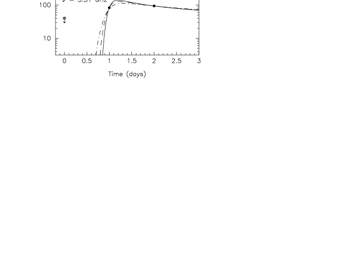
Figure 2: The temporal evolution of the fluxes at 1.41 GHz and 3.31 GHz for the radio flare of GRS 1915+105 observed by Nancy telescope between July 8.0 and July 10.0, 1996 (Gerard 1996), calculated for 3 different expansion speeds: $v_{0}=0.2\,c$ (solid curves), $0.15\,c$ (dashed curves), and $0.1\,c$ (dot-dashed curves). Correspondingly, 3 different ejection times – July 8.8, July 8.73, and July 8.6, are supposed to fit the fluxes detected (full dots) at 3.31 GHz on July 9.0 and July 10.0. The instant $t=0$ corresponds to July 8.0. The open dots show the flux upper limits on July 8 and July 9.

In order to show that such high expansion speed of radio clouds is a common feature for the flares of GRS 1915+105, in Fig. 2 we present evolution of the fluxes calculated for the flare observed on July 8-10 (Gerard 1996), when between July 9 and July 10 apparent transition of the spectra in $1.4-3.3\,\rm GHz$ band from optically thick to thin forms has occured. All curves in Fig. 2 are normalized to the flux $94\,\rm mJy$ at $3.31\,\rm GHz$ observed on July 10.0 (the time $t=0$ in Fig. 2 corresponds to July 8.0). By appropriate choice of the time of ejection it is possible to explain both the flux $83\,\rm mJy$ detected at $3.31\,\rm GHz$, and the flux upper limit at $1.41\,\rm GHz$ on July 9.0 . However, the flux $140\,\rm mJy$ detected on July 10 at $1.41\,\rm GHz$ can be explained only assuming high speed of expansion of radio clouds. As it follows from Fig. 2, for $v_{0}=0.2\,c$ and $0.15\,c$ there is a good agreement between the observed and calculated fluxes, whereas in the case of $v_{0}=0.1\,c$ the calculated flux $S_{\rm 1.4\,GHz}\simeq 105\,\rm mJy$ is significantly below of the $\pm 20\,\rm mJy$ flux error limits for the Nancay measurements (see Rodriguez et al. 1995). In Fig. 2 the magnetic field at the time $t_{0}=1\,\rm day$ is $B_{0}=0.35\,\rm G$, which corresponds to the equipartition field for this flare. Decreasing $B_{0}$ down to $\sim 0.02\,\rm G$, when $w_{\rm e}/w_{\rm B}\geq 10^{5}$ (!), it is possible to fit the measured fluxes with $v_{0}\simeq 0.1\,c$, but not significantly less than that. Thus, even for relatively weak flares one has to suppose very high speeds of expansion of radio clouds, $v_{0}\simeq(0.1-0.2)\,c$.

4.1.2 Magnetic field

Accurate numerical calculations confirm the estimates in Section 2 for the equipartition magnetic field $B_{\rm eq}\sim(0.2-0.3)\,\rm G$ at times of flare maximum, as well as the fact of fast increase of the ratio $\eta=w_{\rm e}/w_{\rm B}$ and required initial injection power $P_{\rm inj}=m_{\rm e}c^{2}\,\int\gamma\,Q_{0}(\gamma){\rm d}\gamma$ of relativistic electrons in the case of $B_{0}<B_{\rm eq}$. For example, the fluxes corresponding to the case of $v_{0}=0.2\,c$ in Fig. 1 require $P_{\rm inj}=1.2\times 10^{38}\,\rm erg/s$ (in the energy range $\gamma\leq 10^{4}$) if $B_{0}=0.2\,\rm G$, and $P_{\rm inj}=10^{39}\,\rm erg/s$ if $B_{0}=0.05\,\rm G$. Note that for a fixed $B_{0}\,$, but different values of other model parameters the values of $P_{\rm inj}$ may change, within factor of $\sim 3$, due to different rates of adiabatic and escape losses. Thus, for the fluxes shown in Fig. 1 in the case of $B_{0}=0.2\,\rm G$, but $v_{0}=0.1\,c$, the injection power $P_{\rm inj}=4.9\times 10^{37}\,\rm erg/s$ is needed.

In Fig. 3 we show the temporal evolution of the fluxes calculated for a fixed $B_{0}=0.2\,\rm G$ but 3 different values of the power-law index $m$ in equation (34), and assuming that electron escape is negligible. One might conclude from Fig. 3 that for proper interpretation of the observed decline of $S_{\nu}(t)$ the index $m$ is to be about $1.2-1.3$. However, the upper panel in Fig. 3 clearly shows that without energy-dependent escape there is no spectral steepening of the fluxes at later stages of the flare, as observed. The dotted curve in Fig. 3, which is calculated for $m=1$ assuming energy-dependent escape, shows noticeable, but still insufficient, evolution of the spectral index $\alpha_{\rm r}$. Simultaneously, the decline of radio fluxes becomes faster, and now well agrees with the observed slope of $S_{\nu}(t)$. Thus, most probably, the decrease of magnetic field in the expanding clouds occurs with the power-law index $m\simeq 1$. Interestingly, for this value of $m$ one could expect that during the cloud’s expansion the ratio $\eta=w_{\rm e}/w_{\rm B}$ remains at some fixed level, $\eta(t)\sim\,\rm const$. Indeed, the magnetic field energy density in a cloud, expanding with some mean $\overline{v_{\rm exp}}$, is decreasing $\propto t^{-2m}$, while the time behavior of the energy density of relativistic electrons can be roughly estimated as $w_{\rm e}\propto\overline{q}\,t/R^{3}\propto t^{-2}$, so $\eta\propto t^{2(m-1)}\sim\,\rm const$. A slow decline of $\eta(t)$ could be expected due to escape of the electrons. Numerical calculations support this conclusion.

4.1.3 Time profiles of the expansion/injection and escape rates

Although the dotted curve in Fig. 3 reveals noticeable steepening of the radio spectrum, it does not explain the spectral index $\alpha_{\rm r}\simeq 0.84$ measured on April 16 (MR94). Our attempts to fit the observed spectra with a constant speed of cloud’s expansion, $v_{\rm exp}(t)=\,\rm const$, failed. As we discussed in Section 3.3, the energy dependent escape of relativistic electrons may result in significant steepening of $N(\gamma,t)$ only on timescales $t\gg\tau(\gamma,t)$. Meanwhile, the spectral index $\alpha_{\rm r}\sim 0.5$ on March 24 implies $\tau(\gamma,t)\geq t$ at $t\simeq t_{0}$. Then, for the escape time given by equation (38), it is difficult to expect sufficiently fast increase of the ratio $t/\tau$ on timescales of few times $t_{0}$, if the cloud would expand with a constant speed.

In order to enable a faster escape of the electrons, one has to assume that expansion of the clouds at times $t\geq t_{0}$ significantly decelerates, which implies $t_{\rm exp}\leq t_{0}^{\prime}$. Simultaneously, the injection rate of relativistic electrons should also decrease, since otherwise due to a slower drop of the magnetic field in time (for decelerated expansion) the decline of $S_{\nu}(t)$ would be significantly slower than observed. The study of possible correlations of the model parameters in Eqs. (32) and (35) which could explain the evolution of both $S_{\nu}(t)$ and $\alpha_{\rm r}(t)$, reveals that the best fits are reached when $t_{\rm exp}\sim$ few days, $k\sim(0.7-1)$, and more importantly, when the time profiles of the injection rate and the speed of expansion are connected with equations $p\simeq 2\,k$ and $t_{\rm inj}\sim(1-2)\,t_{\rm exp}\,$. In Fig. 4 we show the spectra calculated for $t_{\rm exp}=2\,\rm days$ and $k=0.75$, assuming different combinations of the ratios $t_{\rm inj}/t_{\rm exp}$ and $p/k$. Note that for both curves corresponding to $p=2k$ (solid and dotted lines) it is possible to reach a better agreement with the observed slope of $S_{\nu}$ by a better choice of $C_{\lambda}$ or $u$. Meanwhile, in the cases of $p=k$ and $p=3k$ (dashed and dot-dashed curves) the discrepancy between the calculated and measured fluxes may be reduced only if one assumes $t_{\rm inj}\ll t_{\rm exp}$ for $p=k$, or $t_{\rm inj}\gg t_{\rm exp}$ for $p=3k$ . Actually, it would correspond to simulation of the relation $p\simeq 2k$ by means of changing the ratio between $t_{\rm inj}$ and $t_{\rm exp}$ for $q(t)$ and $v_{\rm exp}(t)$.

For the escape rate, the calculations show that generally the value of parameter $C_{\lambda}$ in equation (38) may vary in the range of $(0.1-1)$, and the power-law index $u$ should be $\sim 1.5$, which is somewhat larger than $2m-1\simeq 1$. As discussed above, it implies that the turbulent energy density in the expanding ejecta decreases faster than $w_{\rm B}$.

Thus, the model parameters can be fixed as follows: $\alpha_{\rm inj}\approx 2$, $\Delta\approx 1$, $m\approx 1$, the expansion speed $v_{0}\simeq(0.1-0.3)\,c$, depending on $B_{0}\simeq(0.03-0.3)\,\rm G$ at the time $t=t_{0}$, the characteristic expansion time $t_{\rm exp}\sim$ few days (in the cloud’s rest frame), $t_{\rm inj}\sim 1.5\,t_{\rm exp}$, and $p\simeq 2k$ with $k\simeq(0.7-1)\,$.

4.2 Injection powered by a beam in the jet region ?

The relation $p\simeq 2k$, with $t_{\rm inj}\sim 1.5\,t_{\rm exp}$, implies an interesting interpretation for the primary source of power for continuous injection/acceleration of relativistic electrons. Namely, this kind of temporal behavior of $q(t^{\prime})$ corresponds, in particular, to a scenario when the power $p_{\rm inj}$ of relativistic electrons injected into the cloud per unit surface area decreases with time as $p_{\rm inj}\propto(t{{}^{\prime}})^{-2}$. Then at initial stages, when the cloud expands with a constant speed $v_{\rm exp}(t^{\prime})\simeq v_{0}$, the injection rate $q(t^{\prime})\propto R^{2}p_{\rm inj}=\,\rm const$. At times $t^{\prime}\sim t_{\rm exp}$, when the expansion starts to decelerate, $q(t^{\prime})$ also starts to decline. As follows from equation (33), at times $t^{\prime}\gg t_{\rm exp}$ the radius $R(t^{\prime})\propto(t^{\prime}/t_{\rm exp})^{1-k}$ for $k<1$, and $R(t^{\prime})\propto ln(t^{\prime}/t_{\rm exp})\sim\,\rm const$ for $k=1$. Therefore, in the case of $k\leq 1$, the total injection power at $t^{\prime}\gg t_{\rm exp}$ will be $q(t^{\prime})\propto(t^{\prime}/t_{\rm exp})^{-2k}$, i.e. $p=2k$ as needed. Interestingly, it is possible to understand also, why $t_{\rm inj}$ in equation (35) is somewhat larger than $t_{\rm exp}$: an expanding cloud needs some time of order of $\Delta t^{\prime}\sim t_{\rm exp}$ after the beginning of deceleration for a significant deviation of $R(t^{\prime})$ from the linear behavior, $v_{0}\,t^{\prime}\,$. This interpretation of the time profile of $q(t^{\prime})$ suggests an injection function in the form

$$q_{\rm b}(t^{\prime})=R^{2}(t^{\prime})/(v_{0}t^{\prime})^{2}\;.$$ (39)

Although the discussion above related to $k\leq 1$, the time evolution of radio fluxes observed during the March/April 1994 flare can be explained with the injection rate given by equation (39) even for the values of $k$ somewhat larger than $1$. In Fig. 5 we present the fluxes calculated for the injection rate $q_{\rm b}(t^{\prime})$ for a fixed $t_{\rm exp}$, assuming 3 different values of the index $k$ in the range $(0.7-1.3)$. The values of $v_{0}$ are chosen so as for different $k$ the cloud’s radius $R_{0}$ is the same. Then in all 3 cases the spectral indexes $\alpha_{\rm r}$ at the instant $t_{0}$ practically coincide.

Remarkably, the decline of the specific injection rate $p_{\rm inj}\propto t^{-2}$ suggests a scenario where the injection of electrons is powered by a conically beamed continuous flux of energy from the central engine. Such a beam may be supposed in the form of relativistic wind of magnetized relativistic plasmas and/or electromagnetic waves (Poynting flux) propagating in the conical jet region. Then the energy flux density on the surface of a cloud departing from the central source at a constant speed $\beta$ would decrease $\propto t^{-2}$, as long as the total energy flux propagating in the jet were on a constant level. In this scenario the relativistic electrons may be supposed either directly supplied by the beam, or they may be accelerated on the reverse shock front terminating the wind, or both of these possibilities. Here we would notice that the most probable scenario for explanation of relativistic electrons in the Crab Nebula up to $10^{15}\,\rm eV$ implies their acceleration on the reverse shock, at a distances $\sim 0.1\,\rm pc$, which terminates the ultrarelativistic magnetized wind of (predominantly) $e^{+}-e^{-}$ plasma produced by the pulsar (e.g. Kennel & Coroniti 1984; Arons 1996).

Note that in the framework of the scenario where the bow shock ahead of the ejecta is supposed to be responsible in-situ acceleration of radio electrons, interpretation of $p_{\rm inj}\propto t^{-2}$ law is not so straightforward, especially if one takes into account that the ejecta detected during the March/April flare of GRS 1915+105 did not show any noticeable deceleration. However, we cannot exclude such a possibility, which would require a detailed study, involving a spatial profiles of the density and temperature distributions of the ambient gas. Nevertheless, for convenience further on we will refer to equation (39) as to the case of ”beam injection”, and will use this injection profile which allows us to reduce the number of free model parameters.

4.3 Pair of radio clouds

So far we considered the temporal evolution of the total fluxes of the March/April 1994 radio flare of GRS 1915+105. Below we discuss what kind of information can be found in the radio data when both approaching and receding radio components are resolved, as it is the case for GRS 1915+10 (MR94), as well as for the second of presently known superluminal jet microquasar GRO J1655-40 (Tingay et al. 1995; Hjellming et al. 1995).

4.3.1 Flux ratio: an asymmetry between ejecta

When the pair of oppositely moving radio clouds can be resolved, then in addition to the equation for the observed angular speed $\mu_{\rm a}$ of the approaching cloud, two more equations become available, namely, the equation for the angular speed of receding cloud $\mu_{\rm r}$, and the equation for the ratio of the flux densities detected from two sources. The first two equations are well known, and in general case, allowing for the parameters of the ejecta to be different, for a source at a distance $d$ they can be written as

$$\mu_{\rm a}=\frac{\beta_{\rm a}\sin\theta_{\rm a}}{1-\beta_{\rm a}\cos\theta_{\rm a}}\,\frac{c}{d}\;\;,$$ (40)

$$\mu_{\rm r}=\frac{\beta_{\rm r}\sin\theta_{\rm r}}{1+\beta_{\rm r}\cos\theta_{\rm r}}\,\frac{c}{d}\;\;,$$ (41)

where $\beta_{\rm a,r}$ and $\theta_{\rm a,r}$ are the speeds and the angles of propagation of the approaching and receding ejecta. Note that for convenience in equation (41) we have substituted $\theta_{\rm r}\rightarrow 180^{\circ}-\theta_{\rm r}$, so that $\theta_{\rm a}=\theta_{\rm r}$ for the ejecta moving in strictly opposite directions.

The equation for the flux ratio of the counter jets being considered, it should be said that usually it is supposed in the form of equation (1), where the index $j=3$ for the flux ratio expected from the pair of discrete radio clouds, while the value of $j=2$ gives the brightness ratio of continuous stationary jets, both at equal angular separations $\phi_{\rm a}=\phi_{\rm r}$ from the core (e.g. Lind & Blandford 1985). Note, however, that equation (1) is valid only if the jets are absolutely identical, which implies $\beta_{\rm a}=\beta_{\rm r}=\beta$ and $\theta_{\rm a}=\theta_{\rm r}=\theta$, as well as equal intrinsic luminosities $L_{\rm a}^{\prime}=L_{\rm r}^{\prime}$ of the jets. In this case Eqs. (1), (40) and (41) are not independent, and predict that $(S_{\rm a}/S_{\rm r})_{\phi}=(\mu_{\rm a}/\mu_{\rm r})^{j+\alpha_{\rm r}}$. Then, for the observed values of $\mu_{\rm a}=17\pm 0.4\,\rm mas/day$, $\mu_{\rm r}=9.0\pm 0.1\,\rm mas/day$ and $\alpha_{\rm r}=0.84\pm 0.04$ (MR94), in the case of moving radio clouds ($j=3$) one would expect the flux ratio $(S_{\rm a}/S_{\rm r})_{\phi}=13.1\pm 1.7$, whereas $S_{\rm a}/S_{\rm r}=8\pm 1$ is observed. Remaining in the framework of assumption of identical jets, this discrepancy between the observed and expected flux ratios of the pair of ejecta in GRS 1915+105 can be explained (Bodo & Ghisellini 1995) only if the real speed of radio-emitting plasma (fluid) in the jets would be different from the speed $\beta\simeq 0.92$ of the observed radio patterns attributed, in that case, to propagation of the shocks in the fluid.

Meanwhile, it is possible to explain the observed flux ratio in terms of pattern speeds coinciding with the speeds of the radio clouds, if we suppose that the twin ejecta are similar, but not absolutely identical, allowing for some asymmetry between them (Atoyan & Aharonian 1997). An asymmetry between the ejecta implies validity of at least one of the inequalities $L_{\rm a}^{\prime}\neq L_{\rm r}^{\prime}\,$, $\theta_{\rm a}\neq\theta_{\rm r}\,$, or $\beta_{\rm a}\neq\beta_{\rm r}\,$. Using the relation $S(\nu)=\delta^{3+\alpha_{\rm r}}\,S^{\prime}(\nu)$ between the apparent and intrinsic fluxes of a relativistically moving plasmoids, instead of equation (1), we can write the equation for the flux ratio of the pair of plasmoids at equal intrinsic times

$$\left(\frac{S_{\rm a}}{S_{\rm r}}\right)_{t^{\prime}}\equiv\frac{S_{\rm a}}{S_{\rm r}}=\left(\frac{\Gamma_{\rm r}}{\Gamma_{\rm a}}\right)^{3+\alpha_{\rm r}}\left(\frac{1+\beta_{\rm r}\cos\theta}{1-\beta_{\rm a}\cos\theta}\right)^{3+\alpha_{\rm r}}\,\frac{L_{\rm a}^{\prime}}{L_{\rm r}^{\prime}}\;,$$ (42)

where $\Gamma_{\rm a,r}=1/\sqrt{1-\beta_{\rm a,r}^{2}}$ are the Lorentz factors of bulk motion of the ejecta.

Since a directly measurable quantity is the ratio $(S_{\rm a}/S_{\rm r})_{\phi}$ at equal angular separations $\phi_{\rm a}=\phi_{\rm r}=\phi$, using which the flux ratio $S_{\rm a}/S_{\rm r}$ at equal intrinsic times $t_{\rm a}^{\prime}=t_{\rm r}^{\prime}=t^{\prime}$ can be deduced, the relation between these two flux ratios is to be found. In the frame of observer the ratio of times corresponding to equal angular separation of the sources from the core is $(t_{\rm a}/t_{\rm r})_{\phi}=\mu_{\rm r}/\mu_{\rm a}$, while the ratio of apparent times $t_{\rm a,r}=t^{\prime}/\delta_{\rm a,r}$ corresponding to the same intrinsic time $t^{\prime}$ is $(t_{\rm a}/t_{\rm r})_{t^{\prime}}=\delta_{\rm r}/\delta_{\rm a}$. Using equations (40) and (41), the relation between the ratios of the apparent times corresponding to equal angular separations and equal intrinsic times is found:

$$\left(\frac{t_{\rm a}}{t_{\rm r}}\right)_{\phi}=\Lambda\,\left(\frac{t_{\rm a}}{t_{\rm r}}\right)_{t^{\prime}}\;\;,$$ (43)

where

$$\Lambda=\frac{\Gamma_{\rm r}\,\beta_{\rm r}\,\sin\theta_{\rm r}}{\Gamma_{\rm a}\,\beta_{\rm a}\,\sin\theta_{\rm a}}\;\;\cdot$$ (44)

Then, for the power-law approximation of temporal evolution of the fluxes $S_{\rm a,r}\propto t^{-\kappa}$, the relation between the flux ratios at equal intrinsic times and equal angular separations reads

$$\frac{S_{\rm a}}{S_{\rm r}}\,=\,\Lambda^{\kappa}\,\left(\frac{S_{\rm a}}{S_{\rm r}}\right)_{\phi}\;\cdot$$ (45)

Thus, in the case of symmetrical jets these two ratios coincide, as expected. But generally they are somewhat different, depending on the parameters of the asymmetrical ejecta, which can be derived from the system of equations (40)–(42) for a given flux ratio at equal intrinsic times $S_{\rm a}/S_{\rm r}$, which then can be compared with the measured ratio $(S_{\rm a}/S_{\rm r})_{\phi}$.

Analytical solutions to equations (40)–(42) are found and discussed in detail elsewhere (Atoyan & Aharonian 1997). Due to strong dependence of the ratio $S_{\rm a}/S_{\rm r}$ on the ratio of Lorentz-factors of the bulk motion $\Gamma_{\rm a}/\Gamma_{\rm r}$, equation (42), even the flux ratio $S_{\rm a}/S_{\rm r}\sim 6$ can be easily explained with a very small difference in the speeds of propagation of counter ejecta $\beta_{\rm a}$ and $\beta_{\rm r}$ (see Fig. 6). This implies that an asymmetry in the speeds of ejecta can be considered as the prime reason for the discrepancy between the measured and ‘expected’ flux ratios in GRS 1915+105, although some asymmetry in the intrinsic radio luminosities $L_{\rm a}^{\prime}$ and $L_{\rm r}^{\prime}$, due to somewhat different content of relativistic electrons and/or magnetic fields in the clouds, is possible as well. Any significant difference in the angles of propagation $\theta_{\rm a}$ and $\theta_{\rm r}$ is less probable (at least, the ejecta move in strictly opposite directions on the sky, see MR94).

In Fig. 7 we show the time evolution of the fluxes which could be expected from the approaching (south) and receding (north) radio clouds, in the case of 3 different flux ratios at equal intrinsic times: $S_{\rm a}/S_{\rm r}=7,\;9$ and 13. It is seen, that although the total fluxes (as previously, normalized to the flux observed on March 24) in all cases coincide, the south-to-north partition of these fluxes is essentially different, and for the flux ratio $S_{\rm a}/S_{\rm r}=7$ rather good agreement of the calculated fluxes with the ones detected from both ejecta is reached. The parameters of the bulk motion of approaching and receding ejecta in that case are equal to $\beta_{\rm a}=0.926$, $\beta_{\rm r}=0.902$ and $\theta=70.2^{\circ}$, resulting in the Doppler factors $\delta_{\rm a}=0.55$ and $\delta_{\rm r}=0.33\,$. From equation (45) follows (for the index $\kappa\simeq 1.3$ deduced from observations, MR94) that the flux ratio $S_{\rm a}/S_{\rm r}=7$ at equal intrinsic times of the clouds corresponds to the flux ratio at equal angular separations $(S_{\rm a}/S_{\rm r})_{\phi}=8.6$, which is in agreement with the measured flux ratio $(S_{\rm a}/S_{\rm r})_{\phi}=8\pm 1$.

4.3.2 Synchronous afterimpulses far away from the core ?

It is seen from Fig. 7 that all data points for the total flux of the ejecta, except for the last one (on April 30), deviate from the calculated total flux no more than $10\,\%$, which is not too far from the reported accuracy $\sim\!5\,\%$ of the fluxes measured by the VLA telescopes (MR94). The excess $\sim\!25\,\%$ of the total flux on April 30 could be also explained, if one takes into account the second ejection event occurred around April 23 (see MR94). Meanwhile, when we separate the fluxes measured from the south and north ejecta, the agreement becomes much worse. In particular, this relates to the fluxes of both components on April 9 (corresponding to $t=21\,\rm days$), and to the flux of receding component on April 16 (i.e. $t=28\,\rm days$). Changing a little the model parameters, e.g. assuming a faster escape of the electrons, it is possible to reach a better agreement with the flux measured from the receding cloud on April 9. However, the discrepancy $\sim\!(30-40)\,\%$ for the two other data points cannot be reduced in that way, so another explanation of these fluxes is needed.

We would like to believe that this discrepancy is connected with a significant increase of the fluxes between April 4 and 5 detected by the Nancay telescope. It is seen from Table 1 in Rodriguez et al (1995), that during 24 hours between these 2 days, corresponding to $t=16-17\,\rm days$ after the ejection event, the fluxes at both $1.41\,\rm GHz$ and $3.3\,\rm GHz$ have suddenly increased by $\sim 30\,\%$. Although the VLA was not observing GRS 1915+105 on that days, the ‘echo’ of that increase could be present in the flux detected by VLA from the approaching component on the next observation date, on April 9. The flux from the receding component being considered, one should expect a significant delay between the times of observations of that event from the south and north radio clouds, if this increase was due to a powerful bidirectional afterimpulse from the central source which would have reached the two clouds at equal intrinsic times $t_{\rm a}^{\prime}=t_{\rm r}^{\prime}=t^{\prime}$, and therefore, at different apparent times $t_{\rm a}=t^{\prime}/\delta_{\rm a}$ and $t_{\rm r}=t^{\prime}/\delta_{\rm r}$. In Fig. 8 we show the fluxes calculated for practically the same model parameters as in Fig. 7, but assuming that there was an additional short impulse of injection of relativistic electrons into both clouds during $\Delta t^{\prime}\leq 1\,\rm day$ around intrinsic time $t^{\prime}=9\,\rm days$ after ejection (solid curves). For the calculated Doppler factors of counter ejecta $\delta_{\rm a}=0.55$ and $\delta_{\rm r}=0.33$, this intrinsic time corresponds to the apparent times $t_{\rm a}=16.4\,\rm days$ and $t_{\rm r}=27.2\,\rm days$ for the approaching and receding clouds, respectively, i.e. just between April 4-5 and April 15-16. It is seen from Fig. 8 that the agreement of the calculated fluxes with the measured ones now becomes better. Note that the last two data points (on April 30) in Fig. 8 cannot be explained by another afterimpulse, since they coincide in time. The excess fluxes on that day are, most probably, connected with the second pair of plasmoids ejected around April 23 (see MR94).

If such interpretation of the data is not just an artifact, but corresponds to reality, implications for the physics of jets may be very important. It would mean that both clouds are energized by the central source being even far away from it, at distances $\gg 10^{16}\,\rm cm$ (!), or otherwise we have to rely upon a mere coincidence of equal intrinsic times, as well as amplitudes, of additional injection of relativistic particles from the bow shocks ahead of two counter ejecta, which somehow would impulsively increase the rate of transformation of their kinetic energy to the accelerated electrons. Energization of the clouds from the central source implies that continuous relativistic flux of energy (the beam), in the form of relativistic wind of particles and/or electromagnetic fields, should propagate in the jet region. Then the injection of relativistic electrons into the clouds could be supplied directly through this wind and/or the wind termination reverse shock on the back side of the clouds.

It should be noted, that in principle the excess of the radio fluxes on April 9 and April 16 from approaching and receding clouds, respectively, could be explained also by the synchronous increase of the magnetic fields in both clouds by $\sim 40\,\%$ (the dotted curves in Fig. 8), but not of the injection rate of relativistic electrons. The principle difference between the ‘magnetic’ and ‘electronic’ afterimpulses consists in different behavior of the spectral index $\alpha_{\rm r}$: if the injection of relativistic electrons proceeds smoothly, the spectral index at a given frequency evolves also smoothly, while the ‘electronic’ afterimpulse can result in significant hardening (variations) of the spectral index $\alpha_{\rm r}$. Thus, the data of multi-frequency radio monitoring of the clouds will be able to distinguish between these two options.

Interestingly, some indication for temporary hardening of the radio spectra during April 4 to April 6, i.e. coincident with the time of the supposed ‘afterimpulse’, can be found in the data of observations of the March 19 flare at frequencies 1.41 and 3.28 GHz (Rodrtiguez et al. 1995). This effect can be seen in Fig. 9 where we compare our calculations with all radio data available for the March 19 flare. For the reported accuracy of the Nancy fluxes $\sim 5\,\%\,$ (Rodriguez et al. 1990), the agreement between calculated and measured fluxes at low frequencies is worse than at 8.4 GHz. At these frequencies some allowance is to be made for possible contribution (flickering) of the unresolved central source into the detected total flux, which, in particular, may have significant impact on the correct determination of the power-law spectral index $\alpha_{\rm r}$. Nevertheless, it should be said that while at 8.4 GHz the predicted fluxes well agree with the VLA data, at low frequencies they agree with the measurements only qualitatively, being systematically higher (by $\sim 20\,\%$) than the fluxes measured by Nancy.

Another important feature seen in the Nancy data, is the observed non-smooth decline of the flare, with noticeable variation on timescale of days on the $S_{\nu}\,t$ plot. If not attributed to the flickering of the central source, this may indicate that perhaps the continuous energization of the radio clouds is not as smooth as supposed in our model calculations. Obviously, for interpretation of the multiwavelength radio data with accuracy $\sim 5\,\%$, one needs more accurate theoretical models, which would take into account more complex behavior of the injection and escape of relativistic electrons, as well as the spatial non-homogeneity of the radio clouds.

5 Predictions for nonthermal radiation at high energies

In the study of radio spectra of GRS 1915+105, in the previous sections we did not specify the maximum energies of the accelerated electrons, assuming only that the power-law distribution of the electrons injected into the expanding clouds extend to energies beyond several GeV, to account for the radio flares of GRS 1915+105 detected. Meanwhile, it is not excluded that the relativistic electrons in the jets of microquasars are accelerated to much higher energies, similar to the case of jets in the X-ray selected BL Lacs, where the ultrarelativistic electrons are shown up via the synchrotron X-rays and inverse Compton TeV $\gamma$-rays (e.g. Urry & Padovani 1995; Ghisellini & Maraschi 1997). Therefore, after determination from the radio data the range of model parameters of the ejecta in GRS 1915+105, below we consider the fluxes of the synchrotron and IC radiations which could be expected at higher photon frequences, provided that the spectra of injected electrons would extend beyond TeV energies.

5.1 The synchrotron radiation beyond radio domain

Interpretation of the IR (K-band) jet observed from GRS 1915+105 by Sams et al. (1995) in terms of synchrotron radiation suggests that the injection spectrum of the electrons extends beyond tens of GeV. Besides, the injection of relativistic electrons should continue with rather high rate during the first $t\simeq 10\,\rm days$ or more, which are needed for the ejecta to reach the distances $\gg 10^{16}\,\rm cm$ from the core as observed. The requirement of continuous injection is in agreement with the conclusions derived from radio data, however, there are also some problems, connected with the interpretation of the absolute values of the fluxes of the IR jet.

The reported flux of the IR jet corresponds to the level of maximum radio fluxes observed during the strong flares, extrapolated to the K-band with the power-law index $\alpha_{\rm r}\simeq 0.5$. This typically implies relativistic electrons with power law index $\alpha_{\rm e}\simeq 2$. Meanwhile, although there were no observations in the radio band at the time of detection of the IR jet, typically at $t\geq 10\,\rm days$ after the ejection the radio flares are already at the decreasing stage, when the electron distribution in the GeV range is to be significantly modified, to account for the steep radio spectra at this stage. This is demonstrated in Fig. 10 where by heavy lines we show the temporal evolution of the spectra of electrons in the clouds, calculated so as to provide the flux 655 mJy at 3.5 cm on $t_{0}=4.8\,\rm days$ after ejection, as previously. Note that the flattening of the electron spectra above 10 GeV corresponds to the region where electron escape becomes energy independent, being defined essentially by their flight time across the cloud. In Fig. 11 we show the spectra of synchrotron radiation of these electrons at 3 different times $t$. It is seen that at $t=10\,\rm days$ the synchrotron flux in the IR band is by an order of magnitude less than the flux detected by Sams et al (1996).

To explain the observed high IR flux, we note that the radiation spectra shown by solid curves in Fig. 11, correspond to the emission of relativistic electrons inside the clouds with the mean magnetic field $B(t)$ and radius $R(t)$. Meanwhile, the electrons escaping from the region of high magnetic field, i.e. the cloud, do not immediately disappear, but rather should spend some time at distances comparable with $R$, before departing to large distances from the cloud. In Fig. 10 the thin lines correspond to the energy distribution of the electrons $N^{\prime}(\gamma)$ which have already left the cloud, but still are in the region $\leq 3\,R(t)$. The calculations are done assuming that outside of the cloud the electrons propagate with characteristic radial velocity $\sim\!c/3$ spiraling along the magnetic field lines. The thin lines in Fig. 11 show the synchrotron spectra of those electrons calculated for the magnetic field otside the cloud $B^{\prime}(t)=0.5\,B(t)$. Remarkably, at later stages of the flare the synchrotron radiation flux due to the escaped electrons may be comparable or even exceeding the radiation of the cloud in the IR/optical region, while in the radio domain the radiation produced in the cloud dominates at all timescales. Note that at $t=10\,\rm days$ the total nonthermal IR flux predicted in Fig. 11 is only by factor of $3$ smaller than the one observed.

The results presented in Fig. 11 indicate that the radiation spectra calculated in the framework of more realistic, spatially inhomogeneous, model for the entire synchrotron emission region could be able to explain the steepening of the radio spectra simultaneously with the high IR fluxes much better than the simplified homogeneous cloud model does. Another possibility to increase the flux of synchrotron photons in the IR without contradiction with the observed steepening of the radio spectra, is connected with the assumption of somewhat harder injection spectrum of relativistic electrons, with the power law index $\alpha_{\rm inj}\simeq(1.8-1.9)$.

If the electrons in the jets of GRS 1915+105 are accelerated beyond TeV energies, the contribution of the synchrotron photons may become important also in the X-ray/$\gamma$-ray domain. Most probable origin of the bulk of observed X-rays in this strong X-ray transient source, with the peak luminosities during the flares exceeding $10^{39}\,\rm erg/s$ (e.g. Greiner et al. 1996), is the thermal accretion plasma around the black hole. However, since the observed X-ray spectra are rather steep, with a typical power-law index $\alpha_{\rm x}\simeq 3$ in the region of tens of keV (Harmon et al. 1997), the hard synchrotron radiation of the jets may show up at higher photon energies. It is seen in Fig. 11 that during the first several hours after ejection, when the cloud is still opaque for synchrotron radiation at GHz frequencies, the synchrotron fluxes at energies $\geq 100\,\rm keV$ may dominate over the extrapolation of thermal component. This may result in a significant flattening of the overall spectrum at $E\sim 100\,\rm keV$. Although an existence of such feature in the spectrum of GRS 1915+105 could be seen only marginally (e.g. see Sazonov et al. 1994), in the case of the second microquasar, GRO J1655-40, the X-ray spectra clearly extend up to several hundreds of keV (see Harmon et al. 1995). Interestingly, hard tails of the X-ray spectra are a characteristic feature of other representatives of the population of galactic BH candidates as well, such as Cyg X-1 (Ling et al. 1997) or 1E1740.7-2942 (Churazov et al. 1993; Wallyn et al. 1996). Extending this spectral feature to the extragalactic jet sources, it is worth noting that recently variable hard X-ray spectrum well beyond 100 keV has been detected by BeppoSAX during the recent strong flare of the BL Lac source Mrk 501 (Pian et al. 1997).

5.2 Inverse Compton gamma-rays

Straightforward evidence for acceleration of relativistic electrons beyond TeV energies in the jets of GRS 1915+105 could be provided by detection of the IC $\gamma$-rays at very high energies (VHE), $E_{\gamma}\geq 100\,\rm GeV$. Calculations in the framework of synchrotron-self-Compton model show that during the strong flares one may expect detectable fluxes of VHE $\gamma$-rays, if the magnetic field in the ejected plasmoids would be significantly below of the equipartition level. In Fig. 12 we show the spectra of the synchrotron and IC radiations expected from GRS 1915+105 at $t=0.1\,\rm day$ after the ejection event, calculated for the same model parameters as in Fig. 11, except for somewhat higher exponential cut-off energy, $E_{\rm c}=20\,\rm TeV$, assuming 3 different magnetic fields $B_{0}$ at the instant $t_{0}$. It is seen that for the magnetic field $B_{0}=0.2\,\rm G$, when the ratio of the electron to magnetic energy densities, $\eta=w_{\rm e}/w_{\rm B}$, is at the level close to the equipartition (see Fig. 13), the fluxes of the IC $\gamma$-rays are rather small, whereas assumption of the fields $B_{0}\leq 0.1\,\rm G$ results in a significant increase of the IC $\gamma$-rays .

Such a strong dependence of the expected IC $\gamma$-ray fluxes on the magnetic field is explained by strong dependence of the synchrotron radiation flux on the magnetic field, $S_{\nu}\propto B^{1+\alpha_{\rm r}}$ (e.g., Ginzburg 1979). For magnetic fields smaller by factor of 2, one actually requires an increase of the injection rate of the electrons by factor of $\sim 3$ to provide the same (observed) radio flux. Therefore, assumption of different magnetic fields $B_{0}$ corresponds to assumption of different injection power of relativistic electrons, as shown in Fig. 13. The change of the magnetic field $B_{0}$ has an additional strong impact on the intensity of IC $\gamma$-rays, since for a given field of the soft photons (normalized to the observed radioflux), the increase of the magnetic field by factor of $a$ results in the decrease of the ratio of the photon to magnetic field energy densities by factor of $a^{2}$. Therefore, the share of the injection power of VHE electrons which is channeled into the IC $\gamma$-rays , is essentially reduced.

In Fig. 14 we show the time evolution of the integral fluxes of the IC $\gamma$-rays calculated for the same parameters as in Fig. 11, but for 2 different energies of the exponential cut-off in the spectrum of injected electrons: $E_{\rm c}=20\,\rm TeV$ (solid curves), and $E_{\rm c}=1\,\rm TeV$ (dashed curves). The spectra of the hard X-rays/soft $\gamma$-rays due to synchrotron radiation of electrons in the case of $E_{\rm c}=20\,\rm TeV$ are also shown (dot-dashed curves). The supposed magnetic field $B_{0}=0.05\,\rm G$ requires the ‘beam injection’ power of the electrons $P_{\rm inj}\simeq 4\times 10^{39}\,\rm erg/s$. Fig. 14 shows that in the case of acceleration of the electrons in the ejecta beyond 10 TeV, the synchrotron photons during the flare dominate up to $10\,\rm MeV$ over the flux of IC $\gamma$-rays. The flux of VHE $\gamma$-rays may be on the level of the Crab flux during several hours after ejection of the radio clouds. In a few days the flux drops to the level of 0.1 Crab, which is still detectable by current Imaging Cherenkov telescopes in the Northern hemisphere (CAT, HEGRA, Whipple), but afterwards the source becomes invisible.

Note that this conclusion does not principally change, even if we take into account the contribution due to IC scattering of the electrons after their escape from the cloud (shown in Fig. 14 by thin lines, and calculated under the same assumptions as for Fig. 11), which at these times may become comparable with the flux produced inside of the clouds. The fast drop of the flux of IC $\gamma$-rays is connected with the decrease of the total flux of the background photons, and fast expansion of the clouds, both resulting in a drastic decrease of the density of target photons (most importantly, from the radio to submillimeter domains). Note that contribution due to upscattering of the far IR radiation of the dust, which is possibly present in the vicinity of GRS 1915+105 (Mirabel et al. 1997), remains very small even if the energy density of the dust radiation would be as high as the one of the blackbody radiation, and the radiation temperature be small, $T\sim 100\rm\,K$, which is most favorable for the IC production of the VHE $\gamma$-rays.

The fluence which could be expected at high and very high energies on different timescales during the strong outburst is plotted in Fig. 15. For the Imaging Cherenkov telescopes, with the atmospheric shower collection area $\geq 10^{8}\,\rm cm^{2}$, one could expect up to several tens of $\gamma$-rays with $E\geq 300\,\rm GeV$ during few hours of observations (one night) on the first day of the outburst. In the range of high energies, $E\geq 100\,\rm MeV$, the timescales when the fluxes remain on a high level, do not exceed several hours. For a detector as EGRET aboard of Compton Gamma Ray Observatory, with effective detection area $\sim 10^{3}\,\rm cm^{2}$, the total number of photons expected during that time do not exceed few tens. Meanwhile, for the angular resolution of the EGRET $\sim(3-5)^{\circ}$, the number of background photons above 100 MeV due to diffuse background (Hunter et al. 1997) in the direction of GRS 1915+105 ($l=45.37^{\circ},\;b=-0.2^{\circ}$) during the same time is by factor of 2-3 more. Continuation of the observations beyond the first day cannot noticeably improve the statistics of the high-energy photons due to essential drop of the signal at $t\geq 1\,\rm day$ after ejection (see top panel in Fig. 15). Thus, the EGRET could detect such flares from GRS 1915+105, in the best case, only marginally. However, the future GLAST detector, with 2 orders of magnitude higher sensitivity due to essentially larger effective area and better angular resolution of the photons (e.g. see Bloom 1996), will be able to detect the $\gamma$-ray flares correlated with (or slightly preceding) the radio flares from GRS 1915+105 even if the electrons in the clouds are accelerated only to 10 GeV energy range.

6 Discussion

The data of radio monitoring of the galactic microquasars, which provide a unique opportunity to follow the evolution of the fluxes from the pair of relativistic ejecta on conveniently short time scales, contain large information on the basic parameters and processes in relativistic jets.

The temporal evolution of the radio flares in GRS 1915+105, with apparent transition of the observed fluxes from synchrotron self-absorbed to optically thin spectral forms at the fast rising stage, and later on decline of the fluxes on time scales of days, strongly suggests that the flares are produced in fastly expanding radio clouds ejected from the core (MR94; Rodriguez et al. 1995; Foster et al. 1996). The estimates of the characteristic parameters of the clouds show that in a few days after ejection the clouds should reach the size $R\leq 10^{15}\,\rm cm$, which implies the expansion speeds $\sim(0.1-0.2)\,c\,$ in the rest frame of the ejecta. This estimate is in agreement with the the expansion speed deduced by Mirabel et al. (1997) from the observations of the twin radio plasmoids of 19 March 1994 outburst, and implies extremely large broadening of the emission lines produced, if any, in the clouds, which could effectively prevent their detection in the IR band.

Estimates of the equipartition magnetic field in the clouds result in the values $B_{\rm eq}\simeq 0.2-0.3\,\rm G$ at the stage of maximum of radio flares. The synchrotron cooling time of GeV electrons in such magnetic fields is orders of magnitude larger than characteristic timescale of days during which the radio spectra steepen from the power-law index $\alpha_{\rm r}\sim 0.5$ to $\alpha_{\rm r}\sim 1$. Thus, radiative losses cannot be responsible for this effect. We argue that for explanation of the observed steepening of radio spectra, a continuous injection of relativistic electrons into the radio clouds is needed, the prime reason for the fast modification of the energy distribution of the electrons being the energy dependent escape (due to diffusion and/or drift) of the electrons from the clouds. Note that simultaneous injection and escape of the electrons implies that these two processes proceed from different sides of the cloud, presumably, in the axceal direction for the injection and predominantly transverse direction for the escape.

In the case of magnetic fields close to the equipartition level, $B\simeq B_{\rm eq}$, the energy $W_{\rm B}+W_{\rm el}\sim 10^{43}\,\rm erg$ accumulated in the form of relativistic electrons and magnetic fields in the clouds in a few days after ejection is needed. This implies continuous injection of relativistic electrons with the initial power $P_{\rm inj}\sim 10^{38}\,\rm erg/s$. However, the injection is to be essentially more powerful, $P_{\rm inj}\geq 10^{39}\,\rm erg/s$, if the magnetic fields were smaller than the equipartition field by a factor of $2$ or more. In that case the pressure of relativistic electrons would essentially dominate over the magnetic energy density in the clouds, and could explain, at least qualitatively, fast expansion of the clouds with subrelativistic speeds $v_{\rm exp}\geq 0.1\,c$.

Significant information about the processes in relativistic ejecta in GRS 1915+105 becomes available after detailed comparison of the radio data of the prominent 19 March 1994 outburst (MR94) with the results of accurate model calculations of temporal evolution of the fluxes, produced by relativistic electrons in fastly expanding magnetized clouds. The observed rate of decline of the radio fluxes can be explained if the magnetic field declines with increasing radius of the cloud as $B\propto R^{-m}$ with the index $m\simeq 1$ (see Fig. 3). This implies that the total energy of the magnetic field in the cloud is increasing as $W_{\rm B}\propto R$, so it should be either effectively created in the cloud (presumably, due to turbulent dynamo action) or supplied from outside. Interestingly, a similar dependence of the magnetic field in the conical jet, $B\propto r^{-1}$, but where $r$ is the jet cross-section radius (and not the cloud’s radius, as in our case) have been found by Ghisellini, Maraschi & Treves (1985) for the BL Lac objects. Obviously, these two approximations result in the same behavior of the cloud’s magnetic field on time, $B\propto 1/t$, as long as the cloud expands with a constant speed $v_{\rm exp}(t)\sim v_{0}$, but for timescales $t>t_{\rm exp}$ the decline of $B(t)$ becomes different (slower).

The steepening of the radio spectra from the power-law index $\alpha_{\rm r}\simeq 0.5$ on March 24 to the index $\alpha_{\rm r}\simeq 0.84$ on April 16 can be explained, if both the injection of the electrons and expansion of the cloud would decelerate in a few days after ejection. For interpretation of the temporal evolution of both the spectral index and the fluxes of the March 19 outburst, the model parameters in equations (32) and (35), which describe the time profiles of the expansion speed of the clouds, $v_{\rm exp}(t^{p}rime)$, and of the injection rate of relativistic electrons, $q(t^{\prime})$, should be connected as $t_{\rm inj}\sim(1-2)\,t_{\rm exp}$ and $p\sim 2\,k$, with $k\sim(0.7-1)$ (see Fig. 4). Remarkably, relations of this kind can be provided, if we assume that the electron injection is powered by the continuous beam of energy, in the form of magnetized relativistic wind of particles and/or electromagnetic waves, propagating in the region of conical jet. Fig. 5 shows that the ‘beam injection’ profile $q_{\rm b}(t)$ can readily explain the temporal evolution of the total radio fluxes observed at $8.42\,\rm GHz$ (MR94).

The data of radio monitoring of the pair of counter ejecta in GRS 1915+105 not only allow determination of both the speed $\beta\simeq 0.92$ and angle $\theta\simeq 70^{\circ}$ of propagation of the ejecta (MR94), but also contain principal information of a new quality, which cannot be found in the radio data when only the approaching jet is detected. Indeed, interpretation of the measured flux ratio $(S_{\rm a}/S_{\rm r})_{\phi}\sim 8$ of the pair of radio condensations in terms of a real motion of a pair of radio clouds implies some asymmetry between the intrinsic parameters of the jets in GRS 1915+105. Fig. 6 shows that, e.g., a small difference in the speeds of propagation of the ejecta would be enough to account even for a flux ratio $(S_{\rm a}/S_{\rm r})_{\phi}\sim 6$, which is by factor of 2 smaller than the flux ratio to be expected from identical counter ejecta. Asymmetrical ejection of the pair of plasmoids generally would require, just from the momentum conservation law, a transfer of a significant recoil momentum to the core of ejection, which is the third object in the interacting system ”two jets + core”. Comparison of this momentum with the integrated momentum (absolute values) of the gas orbiting in the inner accretion disk, which is the most probable site responsible for production of relativistic ejecta (e.g., Blandford & Payne 1982; Begelman et al. 1984), suggests (Atoyan & Aharonian 1997) that asymmetrical ejection of pair of plasmoids would be able to induce significant structural changes, or even destruction, of the inner disk, resulting in a temporary reduction/termination of the fuel supply into this region responsible for the thermal X-rays.

Thus, in the framework of this scenario, the onset of subcritical/supercritical accretion would correspond to the active state of the source, with the X-ray flares which can proceed both with and without powerful ejection events and, therefore, observable radio flares (Foster et al. 1996; Tavani et al. 1996). Powerful ejection of the radio emitting material may be accompanied by significant destruction of the inner accretion zone, which may lead to a strong decline of the X-ray fluxes simultaneously with production of relativistic ejecta. The time lag, up to few days, between the decline of the X-ray fluxes and appearance of strong radio flares, as observed in both superluminal microquasars GRS 1915+105 (Foster et al. 1996; Harmon et al. 1997) and GRO J1655-40 (Tingay et al. 1995; Harmon et al. 1995; Hjellming & Rupen 1995), corresponds to the time needed for expansion of the clouds to become optically transparent with respect to synchrotron self-absorption. Depending on the time needed for the recovery of the inner accretion disk after ejection, the radio flares may appear just in the dips between subsequent X-ray flares, as frequently observed (e.g. Harmon et al. 1997).

The data on the radio flux evolution of the pair of resolved ejecta contain important information on the mechanisms of continuous energization of the plasmoids. The interpretation of the $\sim 30\,\%$ excess of the fluxes detected at $8.42\,\rm GHz$ from the approaching and receding ejecta of GRS 1915+105 on April 9 and April 16, respectively, as the result of synchronous short-term increase (‘afterimpulse’) of the injection rate of relativistic electrons into both clouds, as discussed in Section 4, implies continuous energization of the clouds by the central source. Then, the energy is to be supplied up to distances $\geq 3\times 10^{16}\,\rm cm$ by bidirectional beam, presumably in the form of relativistic wind of particles and electromagnetic fields, emerging from the core. Note that the discussed above relations between parameters of the injection rate and cloud’s expansion, which can be provided by the ‘beam injection’ profile given by equation (39), can be regarded as another indication of injection of a real beam into the clouds.

Confirmation of this scenario by future multiwavelength radio observations, if GRS 1915+105 will give us an opportunity to trace another pair of powerful and long lived jets similar to 19 March 1994 event, would suggest significant softening of the enormous energetical requirements rising in the conventional relativistic jet scenario which implies the kinetic energy of the bulk motion of the ejecta be the energy reservoir for in-situ acceleration of the electrons on the bow shocks formed ahead of the ejecta. Indeed, the total energy of the radio electrons injected into the clouds during first few days with the power $P_{\rm inj}\sim 10^{39}\,\rm erg/s$ is about $W_{\rm inj}\sim 3\times 10^{44}\,\rm erg$, and this energy is by a factor of $3$ larger for all duration of the 19 March flare. If this amount of energy were due to kinetic energy of the bulk motion, $W_{\rm kin}$, then the latter would be estimated as at least by another factor of 3 higher than $W_{\rm inj}$, since there was not revealed any deceleration of the bulk motion of the plasmoids beyond April 1994 (see MR94). Thus, $W_{\rm kin}\geq 3\times 10^{45}\,\rm erg$ would be needed. Assuming that this amount of energy is transferred to the bulk motion ‘impulsively’, during a very short timescale (since relativistic speeds imply that in a hundred of seconds the ejecta will be far away from not only the inner accretion disk, but the entire binary), one has to suppose enormous power for acceleration of the ejecta, $P_{\rm jet}\gg 10^{43}\,\rm erg/s$.

Meanwhile, in the scenario which implies continuous energy supply by the beam, the beam power is to be about $P_{\rm inj}$, i.e. comparable with the super-Eddington luminosities observed during the X-ray flares (e.g. Greiner et al. 1996). Moreover, such a beam of relativistic energy can push the cloud forward against the ram pressure of the external medium, therefore at initial stages the plasmoids may move even with some acceleration, until they would acquire enough mass and kinetic energy to continue the flight ballistically. Depending on the parameters of the external medium, the stage of significant acceleration of the ejecta could last, presumably, up to several days, which may be not enough to see this effect. Note that for GRO J1655-40, which is essentially closer to us, the possibility to resolve initial acceleration, perhaps, could be better. Remarkably, in the beam model the acceleration of electrons may occur through the relativistic wind and/or the wind termination shock on the reverse (i.e. facing the central engine) side of the cloud , although a possible contribution due to acceleration on the bow shock ahead of the cloud should not be excluded as well.

Predictions for the fluxes expected beyond radio domain due to synchrotron and inverse Comton radiation mechanisms essentially depend on the maximum energy of accelerated electrons. Assumption of the electrons accelerated beyond 10 GeV would be enough for explanation of the IR jet of GRS 1915+105 observed by Sams et al (1996), and strongly variable IR flares detected by Fender et al (1997). Electrons with energies $\sim 1\,\rm TeV$ produce synchrotron X-rays in the keV band, but even in the case of injection of relativistic electrons with $P_{\rm inj}\sim 3\times 10^{39}\,\rm erg/s$ (this corresponds to $B_{0}\simeq 0.05\,\rm G$), the flux of these photons cannot exceed $\sim\!10\,\%$ of the thermal X-rays of the accretion disk.

However, synchrotron radiation may show up in the range of hard X-rays/soft $\gamma$-rays, if the spectrum of electrons extends to energies $\geq 10\,\rm TeV$. In that case during first several hours (up to 1 day) after the ejection event, the hard synchrotron X-ray fluxes in the range of $E\geq 100\,\rm keV$ could significantly exceed the steep fluxes of thermal X-rays. In the case of $P_{\rm inj}>10^{39}\,\rm erg/s$ (i.e. if the magnetic fields in the clouds are by factor of 2-4 smaller than the equipartition field) the fluxes on the level $I(\geq 100\,\rm keV)>10^{-3}\,\rm ph/cm^{2}s$ can be expected, which could be observed by the detectors like BATSE, SIGMA, OSSE, or BeppoSAX, currently operating in this energy range. Meanwhile, if the magnetic and electron energy densities in the ejecta are about of equipartition, so the injection rate of electrons is $P_{\rm inj}\sim 10^{38}\,\rm erg/s$, then the expected maximum fluxes of the synchrotron X-rays will be smaller by one order of magnitude. Remarkably, even these fluxes will be possible to detect with the forthcoming INTEGRAL mission intended for operation in the energy range $0.1-10\,\rm MeV$. The lack of detection of variable fluxes on the level of $I(\geq 100\,\rm keV)\geq 10^{-4}\,\rm ph/cm^{2}s$ during the first day after ejection event will mean that the maximum (cut-off) energy of relativistic electrons in the ejecta is below TeV domain.

Another, and most straightforward, evidence for TeV electrons in GRS 1915+105 could be provided by detection of VHE $\gamma$-rays. Calculations in the framework of synchrotron-self-Compton model show that during strong flares one may expect detectable fluxes of TeV $\gamma$-rays, provided that the the injection power of relativistic electrons $P_{\rm inj}\geq 10^{39}\,\rm erg/s$ (i.e. magnetic field in the radio clouds significantly below equipartition level). The time evolution of the IC $\gamma$-ray fluxes shown in Figs 14 and 15, predicts that during first several hours of a strong outburst the $\gamma$-ray fluxes above several hundred GeV are on the level of $3\times 10^{-11}\,\rm erg/cm^{2}s$, which corresponds to the level of VHE $\gamma$-ray flux of the Crab Nebula. In a few days the flux drops to the level $0.1\,\rm Crab$ which can be still detected by current Imaging Cherenkov telescopes. Further on, however, the source is not detectable.

Assumption of a lower magnetic field would result in higher fluxes. However, as far as a magnetic fields significantly less than $B_{0}\simeq 0.05\,\rm G$ would imply injection power of electrons $P_{\rm inj}\geq 10^{40}\,\rm erg/s$, it is difficult to expect $\gamma$-ray fluxes essentially exceeding the ones shown in Figs 14 and 15. On the other hand, in the case of in-situ acceleration/injection of the electrons with $P_{\rm inj}\sim 10^{38}\,\rm erg/s$ and magnetic fields on the level of equipartition ($B_{0}\simeq(0.2-0.3)\,\rm G$ at times when $R_{0}\simeq 10^{15}\,\rm cm$), the IC fluxes dramatically decrease. Therefore either positive detection or upper limits of VHE $\gamma$-ray fluxes, being combined with hard X-ray observations above 100 keV, could provide robust constraints on the magnetic fields and efficiency of acceleration of electrons beyond TeV energies.

It is important to note, however, that due to narrow field of view of the Cherenkov telescopes and possibility to do observations only during few night hours per day, the detection of the episodes of VHE $\gamma$-ray emission will be not an easy task. Fortunately, the predicted duration of high fluxes of the VHE $\gamma$-rays is up to few days (see Fig. 15). Then, provided that our interpretation of the observed anticorrelation/delay between strong X-ray and radio flares given above is the case, the instant of a powerful ejection event, and therefore the time (i.e. subsequent first night) most favorable for the VHE observations, can be determined from a strong temporary drop of the thermal X-ray fluxes during the high state of the source. Importantly, occurrence of each strong ejection event can be checked retrospectively by appearance of a strong radio flare which is ‘delayed’ from the time of ejection by 1-3 days.

Information about the IC $\gamma$-rays can be obtained also in the range of high energies, $E\geq 100\,\rm MeV$. It should be noted, however, that even during the first few hours of the flare, the fluxes expected in this energy range do not essentially exceed $10^{-6}\,\rm ph/cm^{2}s$. This implies that in the optimistic case, only marginal detection of such $\gamma$-ray flare can be expected for the EGRET which has effective detection area $\sim 10^{3}\,\rm cm^{2}$ and angular resolution of few/several degrees. We can predict, however, that the future GLAST instrument, with 2 orders of magnitude higher sensitivity than EGRET, will be able to see the $\gamma$-ray flares which would precede, up to few days, strong radio flares from GRS 1915+105.

Acknowledgments   We express our thanks to H. J. Völk for valuable discussions. The work of AMA was supported through the Verbundforschung Astronomie/Astrophysik of the German BMBF under the grant No. 05-2HD66A(7).

References

Arons J., 1996, Space Sci. Rev., 75, 235

Atoyan A. M., Aharonian F. A., 1997, ApJ, 490, L149

Begelman M. C., Blandford R. D., Rees M. J., 1984, Rev. Mod. Phys., 56, 255

Blandford R. D., Payne D. G., 1982, MNRAS, 199, 883

Bloom E. D., 1996, Sp. Sci. Rev., 75, 109

Bloom S. D., Marscher A. P., 1996, ApJ, 461, 657

Bodo G., Ghisellini G., 1995, ApJ, 441, L69

Castro-Tirado A. J., Brandt S., Lund N., Lapshov I., Sunyaev R. A., Shlyapnikov A. A.,

Guziy S., Pavlenko E. P., 1994, ApJS, 92, 469

Churazov E., et al., 1993, A&AS, 97, 173

Fender R. P., Pooley G. G., Brocksopp C., Newell S. J., 1997, MNRAS, in press

(astro-ph/9707317)

Foster R. S., et al., 1996, ApJ, 467, L81

Gerard E., 1996, IAU Circ. 6432

Ginzburg V.L., 1979, Theoretical Physics and Astrophysics, Pergamon, Oxford

Ginzburg V. L., Syrovatskii S. I., 1964, Origin of Cosmic Rays, Pergamon, London

Ghisellini G., Maraschi L., Treves A., 1985, A&A, 146, 204

Ghisellini G., Maraschi L., 1997, in Miller H. R., Webb J. R., eds, Blazar Variability,

PASP (Conf. Ser.), in press

Greiner J., Morgan E. H., Remillard R. A., 1996, ApJ, 473, L107

Harmon B. A., et al., 1994, The second Compton Symposium, AIP Conf. Proc. 304, p.210

Harmon B. A., et al., 1995, Nature, 374, 704

Harmon B. A., Deal K. J., Paciesas W. S., Zhang S. N., Robinson C. R., Gerard E.,

Rodriguez L. F., Mirabel I. F., 1997, ApJ, 477, L85

Hjellming R. M., Rupen M. P., 1995, Nature, 375, 464

Hunter S. D., et al., 1997, ApJ, 481, 205

Kardashev N. S. 1962, Sov. Astron. - AJ, 6, 317

Kennel C. F., Coroniti F. V., 1984, ApJ, 283, 694

Königl A., 1981, ApJ, 234, 700

Landau L. D., Lifshitz E. M., 1963, Electrodynamics of Continuous Media, Pergamon, Oxford.

Liang E., Li H., 1995, A&A, 298, L45

Lind K. R., Blandford R. D., 1985, ApJ, 295, 358

Ling J. C., et al., 1997, ApJ, 484, 375.

Marscher A. P., 1980, ApJ, 235, 386

Meier D., 1996, ApJ, 459, 185

Mirabel I. F., Rodriguez L. F. 1994, Nature, 371, 46

Mirabel I. F., Rodriguez L. F. 1995, Annals NY Academy of Science, 759, 21

Mirabel I. F., Bandyopadhyay R., Charles P.A., Shahbaz T., Rodriguez L. F., 1997,

ApJ, 477, L45

Pacholczyk A. G., 1970, Radio Astrophysics, Freeman, San Francisco

Park B. T., Petrosian V., 1995, ApJ, 446, 699

Pian E., et al., 1997, ApJ, (submitted)

Rodriguez L. F., Gerard E., Mirabel I. F., Gomez Y., Velazquez A., 1995, ApJS, 101, 173.

Sams B. J., Eckart A., Sunyaev R., 1996, Nature, 382, 47

Syrovatskii S. I., 1959, Sov. Astron. -AJ, 3, 22.

Tavani M., Fruchter A., Zhang S. N., Harmon B. A., Hjellming R. N., Rupen M. P., Baylin C.,

Livio M., 1996, ApJ, 473, L103

Tingay S. J., et al., 1995, Nature, 374, 141

Urry M. C., Padovani, P. 1995, PASP, 107, 803

Wallyn P., Ling J. C., Wheaton Wm. A., Mahoney W. A., Radocinski R. G., Skelton R. T.,

1996, A&AS, 120, 295

Figure 1: The spectral fluxes expected from GRS 1915+105 at $t_{0}=4.8\,\rm days$ after ejection of a pair of relativistic plasmoids, $\beta=0.92$, in the case of different magnetic fields $B_{0}$ at the instant $t=t_{0}$ and different expansion speeds $v_{\rm exp}(t^{\prime})=v_{0}$. The curves shown by solid, dashed, and dot-dashed lines correspond to $v_{0}=0.2\,c\,,\;0.1\,c\,,$ and $0.05\,c\,,$ respectively. Other model parameters in Eqs. (32)–(38) are : $m=1$, $\alpha_{\rm inj}=2$, $t_{\rm inj}=20\,\rm days$ ($\gg t_{0}^{\prime}$), and $C_{\lambda}\rightarrow 0$. All curves are normalized to the flux $655\,\rm mJy$ at $\nu=8.42\,\rm GHz$. The fluxes measured by the Nancay and the VLA radio telescopes (Rodriguez et al. 1995) on 24 March 1994 are shown by diamonds and full dots, respectively. The $5\,\%$ error bars for the reported accuracies of these measurements are about of the size of the full dots. Note that the VLA measurements have been done $0.3\,\rm days$ after the Nancay ones. Our calculations, however, show that the fluxes during that short time interval change only by several per cent.

Figure 3: The temporal evolution of the fluxes at 1.41 GHz, 3.28 GHz and 8.42 GHz, and of the spectral index at 8.42 GHz, calculated for 3 different values of the index $m$ in equation (34), assuming negligible escape of the electrons from the cloud which expands with a constant speed $v_{0}=0.2\,c$. The curves plotted by solid, dashed, and dot-dashed lines correspond to $m=1$, $m=1.5$, and $m=0.5$, respectively. The dotted curves are calculated for $m=1$ in the case of significant energy-dependent escape of the electrons, with parameters $\Delta=1$ and $C_{\lambda}=0.5$ in the equation (38). Other model parameters are the for all curves: $B_{0}=0.2\,\rm G$, $\alpha_{\rm inj}=2$, $t_{\rm inj}=20\,\rm days$ and $p=1$. The full squares correspond to the fluxes of the 19 March 1994 flare measured by Nancy telescope (from Rodriguez et al. 1995), and the full dots show the fluxes of the VLA (MR94). $t=0$ corresponds to the supposed time of ejection (March 19.8).

Figure 4: The evolution of the flux $S_{\nu}$ and spectral index $\alpha_{\rm r}$ at 8.42 GHz expected in the case of different relations between the expansion and escape model parameters in equations (32) and (35): $p=2k$ and $t_{\rm inj}=2\,t_{\rm exp}$ (solid lines), $p=k$ and $t_{\rm inj}=t_{\rm exp}$ (dashed lines), $p=3\,k$ and $t_{\rm inj}=2\,t_{\rm exp}$ (dot-dashed lines), $p=2k$ and $t_{\rm inj}=t_{\rm exp}$ (dotted lines). For all cases $k=0.75$ and $t_{\rm exp}=2\,\rm days$ are supposed. Other model parameters are : $\alpha_{\rm inj}=2$, $v_{0}=0.2\,c$, $B_{0}=0.3\,\rm G$, $m=1$, $C_{\lambda}=0.35$, $u=1.5$ and $\Delta=1$.

Figure 5: The evolution of the fluxes and spectral indexes at 8.42 GHz, calculated for the ‘beam injection’ profile of relativistic electrons, $q_{\rm b}(t^{\prime})$, assuming 3 different profiles for the expansion speed $v_{\rm exp}(t^{\prime})$, with the index $k=1$ (solid curves), $k=0.7$ (dashed curves), and $k=1.3$ (dot–dashed curves). In all cases the time $t_{\rm exp}=2.5\,\rm days$, and the initial expansion speeds $v_{0}$ are chosen so as to provide the same radius of the clouds, $R_{0}=7.1\times 10^{14}\,\rm cm$, at the instant $t_{0}=4.8\,\rm days$: $v_{0}=0.15\,c$, $0.135\,c$, and $0.165\,c$, for the solid, dashed, and dot–dashed curves, respectively. The escape parameters $C_{\lambda}=0.25$, $u=1.5$ and $\Delta=1$, and the magnetic field $B_{0}=0.1\,\rm G$ are supposed.

Figure 6: The speeds (bottom panel) and the Lorentz factors (top panel) of the bulk motion of the pair of ejecta calculated for a distance $d=12.5\,\rm kpc$, and angular velocities $\mu_{\rm a}$ and $\mu_{\rm r}$ observed from GRS 1915+105 (MR94), assuming different flux ratios $S_{\rm a}/S_{\rm r}\,$.

Figure 7: The fluxes expected from the approaching (south) and receding (north) radio clouds, in the case of 3 different flux ratios at equal intrinsic times, $S_{\rm a}/S_{\rm r}=7$ (solid curves), 9 (dashed curve), and 13 (dot-dashed curve), calculated under assumption of equal intrinsic luminosities, $L_{\rm a}^{\prime}=L_{\rm r}^{\prime}$, but allowing for the speeds of the bulk motion of the ‘twin’ ejecta to be different, which in these 3 cases are equal to ($\beta_{\rm a}=0.926$, $\beta_{\rm r}=0.902$), ($\beta_{\rm a}=0.923$, $\beta_{\rm r}=0.908$), and ($\beta_{\rm a}=\beta_{\rm r}=0.918$). The clouds expansion speed $v_{0}=0.14\,c$ and escape parameter $C_{\lambda}=0.3$ are supposed. All other model parameters are equal to the ones as in the case of $k=0.7$ in Fig.5. The data points plotted by stars correspond to the total fluxes, and the full dots and full triangles show the fluxes detected by Mirabel & Rodriguez (1994) from the approaching and receding components of the March 19 radio flare. The open dot and open triangle, corresponding to the fluxes 525 mJy and 130  mJy, respectively, are plotted for demonstration of a possible sharing of the 655 mJy total flux between southern and northern components which were not resolved on March 24 (see MR94).

Figure 8: The temporal evolution of the fluxes (bottom panel) expected from the southern and northern radio clouds of the March 19 outburst in the case of synchronous impulsive increase of the injection rate of relativistic electrons (‘electronic afterimpulse’, solid lines) or of the magnetic field (‘magnetic afterimpulse’, dotted lines) in both plasmoids during $\Delta t\leq 1\,\rm day$ around intrinsic time $t^{\prime}=9\,\rm days$ after ejection event. The top panel shows the evolution of the spectral index at 8.42 GHz expected for the southern component. The dashed curves correspond to the case of smooth behavior of the electron injection and magnetic field (i.e., without any afterimpulse). The ‘beam injection’, with the same model parameters as in Fig. 7 (for $S_{\rm a}/S_{\rm r}=7$), is supposed, except for $k=1$ and $C_{\lambda}=0.4$. The error bars on the bottom panel correspond to the $5\,\%$ accuracy of the measured fluxes.

Figure 9: The same as in Fig.8, including the Nancy data at 1.41 GHz and 3.28 GHz (Rodriguez et al. 1995). The dotted curves in this figure show the evolution of the total fluxes and relevant spectral indexes.

Figure 10: Energy distribution of relativistic electrons inside (heavy lines) and outside (thin lines) of the approaching radio cloud at the apparent times $t=0.1\,\rm day$ (solid lines), 1 day (dashed lines), and 10 days (dot-dashed lines). Typical model parameters are supposed: $\alpha_{\rm inj}=2$, $v_{0}=0.2\,c$, $t_{\rm exp}=3\,\rm days$, $k=1$, $\Delta=1$, $u=1.5$, and $C_{\lambda}=0.3$. The magnetic field at the instant $t_{0}=4.8\,\rm days$ is equal to $B_{0}=0.05\,\rm G$, and the exponential cutoff energy for the injected electrons $E_{\rm c}=10\,\rm TeV$.

Figure 11: The spectra of synchrotron radiation, produced inside (heavy lines) and outside (thin lines) of the clouds, by the electrons shown in Fig. 10, at $t=0.1\,\rm day$ (solid lines), $t=1\,\rm day$ (dashed lines), and $t=10\,\rm days$ (dot–dashed lines). The cross and the diamond correspond to the level of maximum fluxes observed during the flares of GRS 1915+105 at $\nu=8.42\,\rm GHz$ and 234 GHz, respectively (Rodriguez et al. 1995). The star shows the flux of the IR jet (Sams et al. 1996), and the hatched region shows the level of the hard X-ray fluxes typically detected from the source in the energy range $\geq 20\,\rm keV$ during the X-ray flares (e.g. Harmon et al. 1997).

Figure 12: The fluxes of the synchrotron (heavy lines) and IC (thin lines) radiations which could be expected from GRS 1915+105 at $t=0.1\,\rm day$ after ejection of a pair of radio clouds, calculated in the case of exponential cut-off energy $E_{\rm c}=20\,\rm TeV$, assuming 3 different values for the magnetic field at the instant $t=t_{0}$: $B_{0}=0.05\,\rm G$ (solid lines) $B_{0}=0.1\,\rm G$ (dashed line), and $B_{0}=0.2\,\rm G$ (dot–dashed lines). All other model parameters are the same as in Fig.11.

Figure 13: The ratios of the electron to the magnetic field energy densities in the expanding plasmoids corresponding to the calculations in Fig.12. Different values of the magnetic field $B_{0}$ at the instant $t_{0}$ (when the cloud’s radius $R=R_{0}\sim 10^{15}\,\rm cm$) actually imply different injection power of relativistic electrons $P_{\rm inj}$. For the supposed $E_{\rm c}=20\,\rm TeV$, the ‘equipartition’ magnetic field corresponds to $B_{0}\simeq 0.3\,\rm G$.

Figure 14: The fluxes of IC $\gamma$-rays expected at different times $t$ from GRS 1915+105 during a strong radio flare in the case of exponential cut-off energy $E_{\rm c}=20\,\rm TeV$ (solid lines) and $E_{\rm c}=1\,\rm TeV$ (dashed lines). The fluxes produced inside and outside of the radio clouds (see text) are plotted by heavy and thin lines, respectively. The dot–dashed curves show the fluxes of synchrotron radiation for $E_{\rm c}=20\,\rm TeV$.

Figure 15: The fluences of the high and very-high energy IC $\gamma$-rays expected during strong radio flares in GRS 1915+105 in the case of 3 different exponential cut-off energies for the accelerated electrons: $E_{\rm c}=20\,\rm TeV$ (solid curves), $E_{\rm c}=1\,\rm TeV$ (dashed curves), and $E_{\rm c}=30\,\rm GeV$ (dot–dashed curve). All other model parameters are the same as in Fig. 11. The supposed magnetic field $B_{0}=0.05\,\rm G$ implies an injection of relativistic electrons with the initial (i.e. at $t\ll t_{\rm inj}$) power $P_{\rm inj}\simeq(3\pm 0.6)\times 10^{39}\,\rm erg/s$, depending on $E_{\rm c}$.