Simulations of non-axisymmetric rotational core collapse

Abstract

We report on the first three-dimensional hydrodynamic simulations of secular and dynamical non-axisymmetric instabilities in collapsing, rapidly rotating stellar cores which extend well beyond core bounce. The resulting gravitational radiation has been calculated using the quadrupole approximation.

We find that secular instabilities do not occur during the simulated time interval of several 10 ms. Models which become dynamically unstable during core collapse show a strong nonlinear growth of non-axisymmetric instabilities. Both random and coherent large scale initial perturbations eventually give rise to a dominant bar-like deformation ($\exp(\pm im\phi$) with $m=2$). In spite of the pronounced tri-axial deformation of certain parts of the core no considerable enhancement of the gravitational radiation is found. This is due to the fact that rapidly rotating cores re-expand after core bounce on a dynamical time scale before non-axisymmetric instabilities enter the nonlinear regime. Hence, when the core becomes tri-axial, it is no longer very compact.

1 Introduction

The rotation rate of a self-gravitating fluid body is usually quantified by the parameter $\beta:=E_{\rm rot}/|E_{\rm pot}|$, where $E_{\rm rot}$ is the rotational energy and $E_{\rm pot}$ the potential energy of the body (e.g., Tassoul 1978). It is well known from linear stability analysis that global non-axisymmetric instabilities can develop in a rotating body when $\beta$ is sufficiently large (e.g., Chandrasekhar 1969; Tassoul 1978). Rotational instability arises from non-radial azimuthal (or toroidal) modes $\exp(\pm im\phi)$, where $\phi$ is the azimuthal coordinate and where $m$ is characterizing the mode of perturbation. The mode with $m=2$ is known as the “bar” mode. Driven by hydrodynamics and gravity, a rotating fluid body becomes dynamically unstable to non-axisymmetric perturbations on a time scale of approximately one rotation period when $\beta>\beta_{\rm dyn}$. Secular instabilities develop due to dissipative processes such as gravitational radiation reaction (GRR; Chandrasekhar 1970), viscosity (Roberts & Stewartson 1963), or a combination of both (Lindblom & Detweiler 1977), and grow on a time scale of many rotation periods (Schutz 1989) when $\beta_{\rm sec}<\beta<\beta_{\rm dyn}$.

The values of the critical rotation parameters $\beta_{\rm sec}$ and $\beta_{\rm dyn}$ depend on the density stratification and the angular momentum distribution of the rotating body. For MacLaurin spheroids, i.e., for incompressible, rigidly rotating equilibrium configurations, secular and dynamical bar instabilities set in for $\beta_{\rm sec}=0.1375$ and $\beta_{\rm dyn}=0.2738$, respectively (e.g., Chandrasekhar 1969; Tassoul 1978). In differentially rotating polytropes ($p\propto\varrho^{1+1/n}$) both the angular momentum distribution and to a lesser extent the polytropic index $n$ affect the value of $\beta_{\rm sec}$ at which the secular bar mode sets in (Imamura et al. 1995). For $n=3/2$ polytropes and $m=2$ perturbations Pickett et al. (1996) find that the classical dynamical stability limit $\beta_{\rm dyn}\approx 0.27$ holds, if the angular momentum distribution is similar to those of MacLaurin spheroids. However, considerably lower values of $\beta_{\rm dyn}$ are found when the latter gives rise to extended Keplerian-disk-like equilibria.

It is unclear to what extent these results obtained analytically for MacLaurin spheroids and numerically for compressible configurations are applicable to collapsing cores, since they are derived for stationary equilibrium models. It has been shown, however, that during axisymmetric rotational core collapse conservation of angular momentum can lead to very rapidly rotating configurations, whose rotation rates exceed $\beta_{\rm sec}$ and even $\beta_{\rm dyn}$ (Tohline 1984; Eriguchi & Müller 1985; Mönchmeyer et al. 1991; Zwerger & Müller 1997). But whether such super-critical rotation in collapsing cores indeed leads to the growth of non-axisymmetric instabilities has not yet been demonstrated in hydrodynamic simulations.

Besides of possibly being relevant for the collapse dynamics of rapidly rotating stellar cores, tri-axial instabilities have also been envisaged to boost the gravitational wave signal from rotational core collapse (for a review, see e.g.,  Piran 1990; Thorne 1995). This would be of great importance for the four long-baseline laser interferometric gravitational wave detectors (GEO600, LIGO, TAMA, VIRGO) which will become operational within the next few years. They are designed to achieve sensitivities (for single bursts) down to gravitational wave amplitudes of $|h|\sim 10^{-22}$ (see e.g., Abramovici et al. 1992). In order to obtain a few events per year, one has to detect all core collapse supernovae out to the Virgo cluster of galaxies (distance $\simeq 10$ Mpc). However, simulations of axisymmetric rotational core collapse predict gravitational wave amplitudes of at most $|h|\sim 10^{-23}$ at that distance (Müller 1982; Finn & Evans 1990; Mönchmeyer et al. 1991; Yamada & Sato 1995; Zwerger & Müller 1997). Significantly larger gravitational wave signals could be produced if non-axisymmetric instabilities due to rotation act in the collapsing core. According to this idea, a rapidly spinning core will experience a centrifugal hang-up and will be transformed into a bar-like configuration that spins end-over-end like an American football, if its rotation rate exceeds the critical rotation rate(s). One has further speculated, that the core might even break up into two or more massive pieces, if $\beta>\beta_{\rm dyn}$ (e.g., Bonnell & Pringle 1995). It has been suggested that the resulting gravitational radiation could be almost as strong as that from coalescing neutron star binaries (Thorne 1995). The actual strength of the gravitational wave signal will sensitively depend on (i) the radius at which the centrifugal hang-up occurs and (ii) what fraction of the angular momentum of the non-axisymmetric core goes into gravitational waves, and what fraction into hydrodynamic waves. These sound and shock waves are produced as the bar or lumps, acting like a twirling-stick, plow through the surrounding mass layers.

Recently, both semi-analytic and numerical methods have been used to compute the gravitational radiation produced by non-axisymmetric instabilities in rapidly rotating stars. Lai & Shapiro (1995) have studied secular instabilities in rapidly rotating neutron stars and have computed the resulting gravitational radiation using linearized dynamical equations and a compressible ellipsoid model. Houser et al. (1994), Houser & Centrella (1996) and Smith et al. (1996) have used three-dimensional hydrodynamic codes to simulate the nonlinear growth of the dynamical tri-axial instability in rapidly ($\beta=0.3$) rotating polytropes ($n=3/2,n=1,n=1/2$). Scaling their results to neutron star dimensions (i.e., a polytrope with mass $M\sim 1.4\,\,{M_{\odot}}$ and radius $R\sim 10$ km) they have also calculated the gravitational radiation from the non-axisymmetric instability. They obtained a maximum dimensionless gravitational wave amplitude $|h|\sim 2\,10^{-22}$ for a source at a distance of 10 Mpc, the energy lost to gravitational radiation being $\Delta E\sim 10^{-3}\,Mc^{2}$.

Concerning investigations, like those just discussed, it is important to note that they can be used to predict the gravitational radiation from rapidly rotating, stationary neutron stars, which might (or might not!) form as a consequence of rotational core collapse. They are not appropriate, however, for predicting the gravitational wave signature of the collapse of rapidly rotating stellar cores. We stress this difference here, because it is often overlooked.

Up to now three-dimensional hydrodynamic simulations of rotational core collapse, which can follow the nonlinear growth of non-axisymmetric instabilities during collapse, have only been performed by Bonazzola & Marck (1993, 1994), and by Marck & Bonazzola (1992). For their simulations they used a pseudo-spectral hydrodynamic code and a polytropic equation of state. They computed the evolution of several initial models and found that the gravitational wave amplitude is within a factor of two of that of 2D simulations for the same initial deformation of the core (Bonazzola & Marck 1994). However, their simulations were restricted to the pre-bounce phase of the collapse, and thus are less relevant.

In the following we report on the first three-dimensional hydrodynamic simulations of non-axisymmetric instabilities in collapsing, rapidly rotating stellar cores which extend well beyond core bounce. In addition to the dynamics, we have also computed the gravitational radiation emitted during the evolution. Our study is a continuation and an extension of the recent work of Zwerger (1995) and Zwerger & Müller (1997), who have performed a comprehensive parameter study of axisymmetric rotational core collapse. The initial models, the equation of state and the hydrodynamic method are adopted from their study. From their set of 78 models we have only considered those which exceed the critical rotation rate(s) during core collapse.

The paper is organized as follows: In section 2 we present the computational procedure used to follow the hydrodynamic evolution of the core and to compute the gravitational wave signal. Subsequently, in section 3, we first discuss the results of a two-dimensional simulation, which serves as a reference point for the three-dimensional runs. We then present various aspects of the evolution of the non-axisymmetric models and discuss the gravitational wave signature of the models. Finally, in section 4, we summarize our results, and conclude with a discussion of the shortcomings of our approach.

2 Computational procedure

2.1 Hydrodynamic method and equation of state

The simulations were performed with the Newtonian multi-dimensional finite-volume hydrodynamic code PROMETHEUS developed by Bruce Fryxell and Ewald Müller (Fryxell et al. 1989). PROMETHEUS is a direct Eulerian implementation of the Piecewise Parabolic Method (PPM) of Colella & Woodward (1984). For the three-dimensional simulations we used a variant of PROMETHEUS due to Ruffert (1992), which utilizes multiple-nested refined equidistant Cartesian grids to enhance the spatial resolution. We do not include any general relativistic effects for the fluid and have neglected effects due to neutrino transport.

Matter in the core is approximated by a perfect fluid using a simplified analytic equation of state (Janka et al. 1993; see also Zwerger & Müller 1997 for details of the implementation). The pressure is a function of the density $\varrho$ and energy density $u$ of the core matter and consists of two parts:

$$P(\varrho,u)=P_{\rm p}+P_{\rm th}\,.$$ (1)

The polytropic part

$$P_{\rm p}=K\cdot\varrho^{\Gamma_{\rm p}}\,,$$ (2)

which depends only on density, describes the pressure contribution of degenerate relativistic electrons or that due to the repulsive nuclear forces at high densities. The thermal part $P_{\rm th}$ mimics the thermal pressure of shock-heated matter. It is computed from the corresponding internal energy density $u_{\rm th}$ by

$$P_{\rm th}=(\Gamma_{\rm th}-1)u_{\rm th},\qquad\mbox{with}\qquad\Gamma_{\rm th}=1.5\,.$$ (3)

The thermal energy density $u_{\rm th}$ in turn is given by the total energy density $u$ through the relation

$$u=u_{\rm p}+u_{\rm th}\,,$$ (4)

where $u_{\rm p}$ is the energy density of the degenerate electron gas. To account for the repulsive part of the nuclear forces the “polytropic” adiabatic exponent $\Gamma_{\rm p}$ (see Eq. (2)) is increased from a value $\Gamma_{1}$ close to $4/3$ (resembling degenerate, relativistic electrons) to a value $\Gamma_{2}=2.5$, if the density of a fluid element exceeds nuclear matter density which is set to $\varrho_{\rm nuc}=2.0\,10^{14}\mathrm{g\,cm}^{-3}$.

2.2 Gravitational wave emission

In the transverse-traceless (TT) gauge a metric perturbation $\@tens{h}$ can be decomposed as (e.g., Misner et al. 1973, chap. 35)

$$\@tens{h}^{\rm TT}=h_{+}\@tens{e}_{+}+h_{\times}\@tens{e}_{\times}$$ (5)

with the unit linear polarization tensors defined, in spherical coordinates $(r,\theta,\phi)$, as

$$\@tens{e}_{+} = \@vec{e}_{\theta}\otimes\@vec{e}_{\theta}-\@vec{e}_{\phi}\otimes\@vec{e}_{\phi}$$

$$\@tens{e}_{\times} = \@vec{e}_{\theta}\otimes\@vec{e}_{\phi}+\@vec{e}_{\phi}\otimes\@vec{e}_{\theta}\,,$$ (6)

where $\@vec{e}_{\theta}$ and $\@vec{e}_{\phi}$ are the unit vectors in the corresponding coordinate directions and $\otimes$ is the tensor product. The two independent polarizations $h_{+}$ and $h_{\times}$ are calculated from the fluid variables in Post-Newtonian approximation, keeping only the mass-quadrupole in the multipole expansion of the field. Let us consider an observer located at coordinates $(r,\theta,\phi)$ in a spherical coordinate system whose origin coincides with the center of mass of the core. Then the two independent polarizations are given by (e.g., Zhuge et al. 1994)

$$h_{+}= {\displaystyle\frac{G}{c^{4}}\frac{1}{r}} \Big{(}\>(\ddot{I}{{\scriptscriptstyle\stackrel{{\scriptstyle-}}{{}}}}_{xx}\cos^{2}\phi+\ddot{I}{{\scriptscriptstyle\stackrel{{\scriptstyle-}}{{}}}}_{yy}\sin^{2}\phi+\ddot{I}{{\scriptscriptstyle\stackrel{{\scriptstyle-}}{{}}}}_{xy}\sin 2\phi)\cos^{2}\theta$$ (7)

$$+\ddot{I}{{\scriptscriptstyle\stackrel{{\scriptstyle-}}{{}}}}_{zz}\sin^{2}\theta-(\ddot{I}{{\scriptscriptstyle\stackrel{{\scriptstyle-}}{{}}}}_{xz}\cos\phi+\ddot{I}{{\scriptscriptstyle\stackrel{{\scriptstyle-}}{{}}}}_{yz}\sin\phi)\sin 2\theta$$

$$-\ddot{I}{{\scriptscriptstyle\stackrel{{\scriptstyle-}}{{}}}}_{xx}\sin^{2}\phi-\ddot{I}{{\scriptscriptstyle\stackrel{{\scriptstyle-}}{{}}}}_{yy}\cos^{2}\phi+\ddot{I}{{\scriptscriptstyle\stackrel{{\scriptstyle-}}{{}}}}_{xy}\sin 2\phi\>\Big{)}$$

$$h_{\times}= {\displaystyle\frac{G}{c^{4}}\frac{2}{r}} \Big{(}\>\frac{1}{2}(\ddot{I}{{\scriptscriptstyle\stackrel{{\scriptstyle-}}{{}}}}_{yy}-\ddot{I}{{\scriptscriptstyle\stackrel{{\scriptstyle-}}{{}}}}_{xx})\sin 2\phi\cos\theta+\ddot{I}{{\scriptscriptstyle\stackrel{{\scriptstyle-}}{{}}}}_{xy}\cos 2\phi\cos\theta$$ (8)

$$+(\ddot{I}{{\scriptscriptstyle\stackrel{{\scriptstyle-}}{{}}}}_{xz}\sin\phi-\ddot{I}{{\scriptscriptstyle\stackrel{{\scriptstyle-}}{{}}}}_{yz}\cos\phi)\sin\theta\>\Big{)}\,.$$

Here the quantities $\ddot{I}{{\scriptscriptstyle\stackrel{{\scriptstyle-}}{{}}}}_{ij}$ are the second time derivatives of the Cartesian components of the reduced quadrupole moment tensor $\@tens{I}{\hskip 1.19995pt{\scriptscriptstyle\stackrel{{\scriptstyle-}}{{}}}}$. They are defined according to

$$\ddot{I}{{\scriptscriptstyle\stackrel{{\scriptstyle-}}{{}}}}_{ij}:=\frac{{\rm d}^{2}}{{\rm d}t^{2}}\int\varrho\left(\@vec{x},t-r/c\right)\cdot\left(x_{i}x_{j}-\frac{1}{3}\delta_{ij}x_{k}x^{k}\right)\,{\rm d}^{3}\@vec{x}\,,$$ (9)

where we have used the Einstein sum convention (i.e.,  summation over repeated indices) and where $\delta_{ij}$ is the Kronecker symbol. Note that the origins of the spherical coordinate system (used to specify the observer’s position) and the Cartesian coordinate system (used to describe the matter distribution of the source) coincide. The coordinate systems are oriented relative to each other such that $\theta=0$ corresponds to the positive $z$-direction.

We assume that the source possesses equatorial symmetry (i.e., it is symmetric with respect to the transformation $z$ $\to$ $-z$), and hence $I{{\scriptscriptstyle\stackrel{{\scriptstyle-}}{{}}}}_{xz}=I{{\scriptscriptstyle\stackrel{{\scriptstyle-}}{{}}}}_{yz}\equiv 0$. Inspection of the remaining terms in Eqns. (7) and (8) then yields $\theta\in\{0,\pi/2\}$ and $\theta=0$ as necessary conditions for extrema of the waveforms $h_{+}$ and $h_{\times}$ (considered as functions of the observer’s position), respectively. Thus, we calculate $h_{\times}$ along the positive $z$-axis and $h_{+}$ in the equatorial plane (at an azimuthal position $\phi=0$) to yield the maximum stresses. We have checked for all models that we do not miss possible additional (short term) maxima of $h_{+}$ that could be present for an observer at some azimuthal position $\phi\neq 0$ in the equatorial plane but could be overlooked by an observer located at $\phi=0$.

The quadrupole part of the total gravitational wave energy is given by

$$E_{\rm GW}=\frac{1}{5}\frac{G}{c^{5}}\int^{\infty}_{-\infty}\dddot{I{\scriptscriptstyle\stackrel{{\scriptstyle-}}{{}}}}_{ij}\dddot{I{\scriptscriptstyle\stackrel{{\scriptstyle-}}{{}}}}_{ij}\,{\rm d}t\,.$$ (10)

Instead of numerically approximating Eq. (9) with standard finite differences, it is superior (e.g., Finn & Evans 1990; Mönchmeyer 1993) to use an equivalent expression derived independently by Nakamura & Oohara (1989) and by Blanchet et al. (1990):

$$\ddot{I}{{\scriptscriptstyle\stackrel{{\scriptstyle-}}{{}}}}_{ij}={\rm STF}\left\{2\noindent\int\varrho\cdot(v^{i}v^{j}-x^{i}\partial_{j}\Phi)\,{\rm d}^{3}\@vec{x}\right\}\,,$$ (11)

where the symmetric and trace free part of a doubly indexed quantity $A_{ij}$ is defined by

$${\rm STF}\{A^{ij}\}:=\frac{1}{2}A^{ij}+\frac{1}{2}A^{ji}-\frac{1}{3}\delta^{ij}A^{ll}\,.$$ (12)

The spatial derivatives $\partial_{j}\Phi$ of the gravitational potential appearing in Eq. (11) are approximated by centered finite differences.

For two reasons no back-reaction of the gravitational wave emission on the fluid (GRR) has been implemented. Firstly, the peak luminosity of gravitational radiation that can be expected from rotational core collapse is at most of the order of $10^{50}$ erg s^-1 (Müller 1982; Finn & Evans 1990; Mönchmeyer et al. 1991; Zwerger & Müller 1997). When comparing this luminosity with the typical energies (kinetic, rotational, potential, internal) $E\simeq 10^{52}$ erg of the core one finds a GRR time scale of the order of 100 s, which is at least by a factor of $10^{4}$ larger than the time interval over which we can calculate the core’s evolution. Secondly, total energy conservation is violated by an amount $\Delta E\simeq 10^{49}$ erg in the best resolved 2D calculation and by an amount $\Delta E\simeq 10^{50}$ erg in the 3D runs. This violation means an acceptable 1%-error as far as the dynamics is concerned. However, it dominates the change of energy radiated due to GRR ($E_{\rm GW}\la 10^{47}$ erg) in the time interval of our simulations by about a factor of $10^{3}$.

2.3 Two-dimensional simulations

Closely following Zwerger & Müller (1997), the axisymmetric (reference) simulations were performed in spherical coordinates assuming equatorial symmetry. Thus, the angular grid covered the range $\theta\in[0,\pi/2]$. The number of equidistant angular zones was $n_{\theta}=18$, 45 or 90, which corresponds to an angular resolution of $5^{\circ}$, $2^{\circ}$ or $1^{\circ}$, respectively. The moving radial grid consisted of 360 zones. The grid was moved in such a way that the inner core (i.e., the subsonic inner part of the core) was always resolved by 180 radial zones. The radial zoning varied from about 0.5 km in the unshocked inner core to about 50 km in the outermost parts of the outer core (for more details see Zwerger & Müller 1997).

As in Zwerger & Müller (1997), the gravitational wave amplitude was computed by expanding the gravitational field into “pure-spin tensor harmonics” (Thorne 1980). The only non-vanishing quadrupole contribution is then given by

$$A^{{\rm E}2}_{20}=\frac{G}{c^{4}}\frac{16\pi^{3/2}}{\sqrt{15}}\,\frac{{\rm d}^{2}}{{\rm d}t^{2}}\int_{0}^{\infty}\int_{-1}^{1}\varrho\left(\frac{3}{2}z^{2}-\frac{1}{2}\right)r^{4}\,{\rm d}z{\rm d}r\,,$$ (13)

which is related to the (dimensionless) metric perturbations of Eq. (5) by

$$h_{+}=\frac{1}{8}\sqrt{\frac{15}{\pi}}\sin^{2}\theta\,\,\frac{A^{{\rm E}2}_{20}}{r}\,,\qquad h_{\times}\equiv 0$$ (14)

Using the counterpart of Eq. (11) in spherical coordinates (e.g., Zwerger & Müller 1997, Eq. 20), the second time derivative as well as the $r^{2}$-weighting of mass elements, both numerically troublesome (e.g., Finn & Evans 1990), can be eliminated.

In the quadrupole approximation the total gravitational wave energy is given by

$$E_{\rm GW}=\frac{c^{3}}{G}\frac{1}{32\pi}\int^{\infty}_{-\infty}\left(\frac{{\rm d}A^{{\rm E}2}_{20}}{{\rm d}t}\right)^{2}\,{\rm d}t\,.$$ (15)

Higher-order terms in the multipole expansion of the gravitational wave field are negligible both for the wave amplitudes and the amount of radiated energy in the axisymmetric case (e.g., Mönchmeyer et al. 1991, Zwerger 1995).

Figure 1: Snapshots of the density distribution (in units of [$\mathrm{g\,cm}^{-3}$]) and the velocity field in a meridional plane for the axisymmetric model A4B5G5. The $z$-axis coincides with the axis of rotation (and symmetry). The contours are logarithmically spaced with intervals of 0.25 dex, they are shaded with darker grey values for higher density regions and labeled with their respective values. The time of the snapshot and the velocity scale are given in the top right corner of each panel.

2.4 Three-dimensional simulations

The three-dimensional calculations have been performed on multiple-nested refined equidistant Cartesian grids (see Ruffert (1992) for details of the method). As in the 2D calculations we assume the equatorial plane $z=0$ to be a plane of symmetry. Six centered grids were used each of which was refined by a factor of two. In direction of the rotation ($z$-) axis each grid had 32 zones, while the perpendicular grid planes consisted of $64\times 64$ zones. The coarsest grid had a spatial extent of 2560 km covering the entire core with cubes of edge size 40 km. The finest grid covered the innermost 80 km with a linear resolution of about 1 km. Thus, the resulting spatial resolution was comparable to that of the 2D simulations.

For the three-dimensional simulations we considered axisymmetric models of Zwerger & Müller (1997), which are stable against non-axisymmetric perturbations in the early stages of collapse (i.e., $\beta(t)\la 0.1$), but later exceed the critical rotation rate(s). Test calculations showed that non-axisymmetric instabilities did not grow in perturbed axisymmetric models with $\beta\la 0.1$ on time scales of a few 10 ms. Using trilinear interpolation an axisymmetric model was mapped onto the three-dimensional grid when its rotation parameter reached a value of $\approx 0.1$. Typically, this occured a few milliseconds before core bounce.

We then imposed certain non-axisymmetric perturbations and followed the subsequent dynamical evolution of the core in three spatial dimensions. Due to the cubic cells of our computational grid, the mapping procedure itself introduces deviations from axisymmetry that are symmetric with respect to the coordinate transformations

$$\phi\to\phi+\pi/2\qquad\mbox{and}\qquad\phi\to\phi+\pi\,.$$ (16)

This implies that only azimuthal modes $\exp(im\phi)$ with even values of $m$ are contained in the “grid-mapping noise”. The amplitudes are of the order of a few percent measured as relative deviations $\delta\psi:=(\psi-\langle\psi\rangle_{\phi})\,/\,\langle\psi\rangle_{\phi}$ of a scalar field $\psi(r,\theta,\phi)$ from its azimuthal mean $\langle\psi\rangle_{\phi}:=(2\pi)^{-1}\,\int_{0}^{2\pi}\psi(r,\theta,\phi)\,{\rm d}\phi$. This defines a lower limit for the size of the perturbation amplitudes, which we can impose explicitly onto the axisymmetric models. We point out that density perturbations $\delta\varrho\simeq 1\%$ are about two orders of magnitude larger than those typically used in numerical stability analysis (e.g., Houser et al. 1994; Aksenov 1996; Smith et al. 1996).

We used explicit random perturbations of the density with an amplitude of 10%, i.e., the density distribution of the mapped model was modified according to

$$\varrho(r,\theta,\phi)\to\varrho(r,\theta,\phi)\,\cdot\,\big{[}1+0.1\,f(r,\theta,\phi)\big{]}\,,$$ (17)

where $f$ denotes a random function distributed uniformly in the interval $[-1,1]$. All azimuthal modes that can be resolved on a given grid are therefore present in the initial data, the $m=4$ and $m=2$ “grid-modes” mentioned above presumably being dominant. The corresponding model is refered to in the following as model MD1.

In a second model MD2, we imposed in addition a large scale $m=3$ azimuthal perturbation with an amplitude of 5%, i.e.,

$$\varrho(r,\theta,\phi)\to\varrho(r,\theta,\phi)\,\cdot\,\big{[}1+0.05\,\sin(0.6+3\phi)\big{]}\,.$$ (18)

Note that for convenience of notation we have given the form of the perturbation in spherical coordinates, although it is introduced on a Cartesian grid.

3 Results

Zwerger & Müller (1997) have studied the overall dynamics of axisymmetric rotational core collapse and calculated the resulting gravitational wave signal. In particular, they have investigated how the dynamics and the gravitational radiation depend on the (unknown) initial amount and distribution of the core’s angular momentum, and on the equation of state. Among the 78 models computed by them, Zwerger & Müller (1997) found only one model (A4B5G5), whose rotation rate parameter considerably exceeds $\beta_{\rm dyn}$ near core bounce. However, $\beta$ remains larger than $\beta_{\rm dyn}$ for only roughly one millisecond, because the core rapidly re-expands after bounce and hence slows down. In addition, Zwerger & Müller (1997) found three more models (A3B5G4, A3B5G5 and A4B5G4) that fulfilled $\beta>\beta_{\rm sec}$ for several 10 ms (see Fig. 4 of Zwerger & Müller 1997).

The two “classical” dissipation mechanisms that can in principle drive secular non-axisymmetric instabilities, namely viscosity of core matter (Roberts & Stewartson 1963) and gravitational radiation reaction (GRR; Chandrasekhar 1970), are negligible during the time scales we have simulated evolution of the core (a few 10 ms). Nevertheless, some inner fraction of the collapsing core could still become unstable, because of acoustic coupling with or due to advection of matter into the outer core (see e.g., Schutz 1983 and references therein). Therefore, we have experimented with two of the three models exceeding $\beta_{\rm sec}$ (but not $\beta_{\rm dyn}$) for several 10 ms by imposing non-axisymmetric perturbations on different hydrodynamic quantities ($\varrho$, $P$, $\@vec{v}$) of different spatial character ($m=2$, random) and amplitude (5%, 10%) at different epochs of the evolution. On a time scale of several 10 ms we have found neither indications for secular instabilities nor a significant enhancement of the gravitational wave signal (compared with the corresponding axisymmetric model).

Thus, the only model remaining of the set of models of Zwerger & Müller (1997), which is a promising candidate for the growth of tri-axial instabilities during its gravitational collapse, is model A4B5G5 (see above). Its properties are described in the next subsection. Some global quantities of the model have already been published by Zwerger & Müller (1997).

Figure 2: Radii of selected mass shells (for their definition see Eq. (20) in the text) as a function of time for two three dimensional models MD1 (dashed lines) and MD2 (dashed-dotted lines), and the axisymmetric model A4B5G5 (solid lines). The mass inside the shown mass shells ranges from $0.1\,{M_{\odot}}$ to $0.9\,{M_{\odot}}$ in intervals of $0.2\,{M_{\odot}}$. Lines corresponding to $0.1\,{M_{\odot}}$ and $0.7\,{M_{\odot}}$ are drawn in bold.

3.1 The axisymmetric model A4B5G5

All pre-collapse models of Zwerger & Müller (1997) are axisymmetric $n=3$ polytropes ($p\propto\varrho^{1+1/n}$) in rotational equilibrium whose angular velocity $\Omega$ only depends on the distance $\varpi$ from the axis of rotation according to the rotation law

$$\Omega(\varpi)\propto\left(1+(\frac{\varpi}{A})^{2}\right)^{-1}\,.$$ (19)

Collapse is initiated by reducing the adiabatic index $\Gamma$ from the value 4/3, which is consistent with the structure of a $n=3$ polytrope, to a somewhat smaller value $\Gamma_{1}$ (see Eq. (2)).

The initial model A4B5G5 is the most extreme one in the large parameter set considered by Zwerger & Müller (1997). It is the fastest ($\beta_{\rm i}=0.04$) and most differentially ($A=10^{7}$ cm; see Eq. (19)) rotating model being evolved with the softest equation of state ($\Gamma_{1}=1.28$). According to the criterion derived by Ledoux (1945; Eq. 77) for rotating stars, a rotation rate of $\beta=0.04$ requires $\Gamma_{1}>1.3$ for the star to be stable against the fundamental radial mode, i.e., collapse. The resulting model has a mass of $1.66M_{\odot}$, a total angular momentum of $L_{z}=3.85\,10^{49}$ erg s and an initial equatorial radius of 1280 km.

Fig. 1a shows that model A4B5G5 has a torus-like density stratification with an off-center density maximum, which is located in the equatorial plane 200 km away from the rotation axis. During collapse a kind of “infall channel” forms along the rotation axis, a structure which has already been found in some models of Mönchmeyer et al. (1991). There matter falls almost at the speed of free-fall towards the center. With decreasing latitude (i.e., increasing polar angle $\theta$) matter is increasingly decelerated by centrifugal forces (Fig. 1b). At $t\approx 28$ ms, which is about 3 ms before core bounce, an oblate shock is visible (Fig. 1c). It begins already to form at the bottom of the infall channel 7 ms before core bounce (Fig. 1b). Pressure gradients decreasing with increasing polar angle $\theta$ lead to an asymmetric propagation of the shock its speed being larger in polar than in equatorial regions. The result is a “prolate shock in an oblate star” (Finn & Evans 1990).

Figure 3: Rotation rate parameter $\beta$ as a function of time for the three-dimensional models MD1 (dashed) and MD2 (dashed-dotted). For comparison, the evolution of $\beta$ of the two-dimensional model is shown, too (solid). The solid horizontal lines mark the critical values $\beta_{\rm sec}$ (lower line) and $\beta_{\rm dyn}$ (upper line), where MacLaurin spheroids become secularly and dynamically unstable to non-axisymmetric bar-like perturbations.

A second shock, which forms at the edge of the torus shortly before the density in the core reaches its maximum value inside the torus, propagates behind the outer shock (Fig. 1d). Like the outer shock, the inner shock eventually becomes prolate, too.

Figure 4: Maximum density on the grid as a function of time for the three-dimensional models MD1 (dashed) and MD2 (dashed-dotted). For comparison we also show the maximum density of the two-dimensional model A4B5G5 (solid). The solid horizontal line marks the assumed nuclear matter density $\varrho_{\rm nuc}=2\,10^{14}\mathrm{g\,cm}^{-3}$.

The overall dynamics of the core can be conveniently analyzed in terms of the radial extent of different “mass shells” $M(R)$ defined by

$$M(R):=2\pi\int_{0}^{R}\int_{0}^{\pi}\langle\varrho(r,\theta)\rangle_{\phi}\,r^{2}\sin\theta\,{\rm d}\theta{\rm d}r\,,$$ (20)

where $\langle\rangle_{\phi}$ denotes the azimuthal mean of the density to be calculated in the 3D simulations. $M(R)$ is the mass contained in a sphere of radius $R$. Note that in more than one spatial dimension these mass shells are not identical with the well known Lagrangian mass shells.

Inverting $M(R)$ one obtains the radius $R_{M}$ of the mass shell. This quantity is plotted as a function of time for different masses $M$ in Fig. 2. One recognizes that maximum compression is reached in model A4B5G5 at $t=30.67$ ms, which is followed by an expansion lasting for about 2 ms. Without any further significant oscillations the inner core evolves towards its new equilibrium: The radii of mass shells with $M\la 0.7\,{M_{\odot}}$ are nearly constant with time for $t\ga 33$ ms (Fig. 2). The same behavior can be deduced from the evolution of the rotation parameter ($\beta\propto R^{-1}$ for a homogeneous sphere with radius $R$) and of the maximum density on the grid (Figs. 3 and 4). Figure 2 also shows that the central core $M(R)<0.7\,{M_{\odot}}$ oscillates with a single dominant volume mode, which is in agreement with the results obtained by Mönchmeyer et al. (1991). They found single volume modes in cores with coherent motion in equatorial and polar directions. This certainly occurs in model A4B5G5, since matter in the torus which contains most of the mass shows almost no motion in polar directions at all.

Figure 5: Snapshots of the density distribution (in units of [$\mathrm{g\,cm}^{-3}$]) in the equatorial plane of model MD1. The contours are logarithmically spaced with intervals of 0.25 dex, they are shaded with darker grey values for higher density regions and labeled with their respective values. The time of the snapshot is given in the upper right corner of each panel.

Matter in the torus (about $0.7\,{M_{\odot}}$) stays in sonic contact, i.e., it contracts coherently. It also remains unshocked well beyond core bounce. Hence, the torus resembles the qualitative features of a homologously contracting inner core that has been found analytically for the spherical collapse of polytropic cores (Goldreich & Weber 1980, Yahil 1983) and numerically in slowly rotating cores with ellipsoidal density stratification (Finn & Evans 1990; Mönchmeyer et al. 1991).

The main features of the quadrupole amplitude $A^{\rm E2}_{20}$ calculated for model A4B5G5 are: A slow monotonic increase with time for the first 25 ms is followed by a pronounced negative spike at the time of bounce with no subsequent short-period oscillations (see Fig. 9). We therefore consider the gravitational waveform to be closest resembled by signal type II, which is characterized by prominent spikes arising at the bounce(s) due to single dominant volume mode(s) (Mönchmeyer et al. 1991).

The non-vanishing polarization, calculated for a source at 10 Mpc and for an observer located in the equatorial plane of the core, has a peak value of $h_{+}=-3.5\,10^{-23}$. The energy of the quadrupole radiation is $E_{\rm GW}=7.8\,10^{-8}\,{M_{\odot}}\,c^{2}$. Most of the spectral power is radiated at a frequency of $\nu\approx 200$ Hz. This is the largest signal strength obtained for any axisymmetric collapse models in the set of Zwerger & Müller (1997). However, the amplitude is still by at least one order of magnitude too small to be detectable even with the “advanced” LIGO interferometer (see Abramovici et al. 1992 for the sensitivity limits), if the source is located in the Virgo cluster.

3.2 Evolution of non-axisymmetric models

The initial non-axisymmetric perturbations were introduced at $t_{0}=28.13$ ms (Figs. 5a and 7a). This is about 2.5 ms before bounce (when the density reaches a maximum inside the torus), and about 2 ms before the core’s rotation rates $\beta\ga 0.3$, i.e., when it should become dynamically unstable. The additional perturbation of 5% amplitude and $m=3$ azimuthal dependence imposed on model MD2 can hardly be distinguished from the 10% random noise perturbations of both models. The inner torus has contracted from an initial radius of 200 km to one of 60 km at $t=t_{0}$. Note that we refer to its density maximum, when we give its radial position.

The subsequent rapid contraction of the rotating core is reflected by a steep rise of the maximum density, which peaks at $t=30.68$ ms in both 3D models and in the axisymmetric one (Fig. 4). At approximately the same time the contraction (Fig. 2), the rotation parameter $\beta$ (Fig. 3), the dissipation-rate of kinetic-infall energy into thermal energy and the gravitational potential energy reach their peak values. Thus, we consider $t=30.68$ ms to be the time of bounce, although the central density does not reach its first peak then, which is usually considered as the bounce criterion. However, because of the torus-like density stratification of the models, the central density has less meaning. During the simulations it remained always much lower than the maximum density inside the torus (by 1 – 3 orders of magnitude). One also has to be careful, in particular in 3D simulations, when deriving implications from “local” quantities. For example, one might be tempted to conclude from the fact that the maximum density exceeds nuclear matter density in model MD2, i.e., $\varrho_{\rm max}>2\,10^{14}\mathrm{g\,cm}^{-3}$ (Fig. 4), that this model contrary to model MD1 suffered a bounce due to the stiffening of the equation of state. However, nuclear matter density is exceeded only in a few zones inside the torus (see Fig. 7c), while the corresponding azimuthal average, which is determining the overall dynamics, is practically identical to that in model MD1. Therefore, we always compare the value of the maximum density with the corresponding azimuthal mean, before drawing any conclusions.

Up to $t\approx 33$ ms, i.e., up to about 2 ms after bounce, the non-axisymmetric initial perturbations have not grown far enough to produce any significant changes in the overall dynamics of the collapsing core. This can be seen by comparing the time evolution of the radii of mass shells defined by Eq. (20) (see Fig. 2). Also locally, non-axisymmetries are still small perturbations on a rapidly changing axisymmetric background. The density contrast in the torus is $\delta\varrho\la 0.15$ for model MD2 at $t\leq 33$ ms (Figs. 7a–c). Hence, the distribution of hydrodynamic variables in planes perpendicular to the rotation axis is still given by Fig. 1.

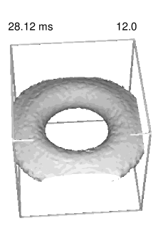
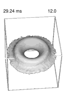
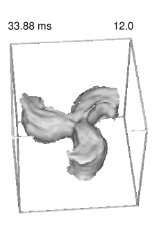
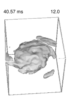
Figure 6: Surfaces of constant density $\varrho=10^{12}\mathrm{g\,cm}^{-3}$ for model MD2. The edges of the cubic box have a length of 160 km. The snapshots are taken at the same times as those in Fig. 7.

Figure 7: Snapshots of the density distribution (in units of [$\mathrm{g\,cm}^{-3}$]) in the equatorial plane of model MD2. The contours are logarithmically spaced with intervals of 0.25 dex, they are shaded with darker grey values for higher density regions and labeled with their respective values. The time of each snapshot is given in the upper right corner of each panel.

The subsequent evolution differs from that of the axisymmetric model and is also different between the two 3D models.

Model MD1: Due to the Cartesian geometry of the computational grid, the toroidal mode with $m=4$ sticks out of the noise first. The inner torus assumes a transient square-like structure, which exists for $\approx 7$ ms. This does not influence the overall dynamics of the model significantly compared to the axisymmetric one, although we find a somewhat less compact density stratification when comparing the radii of the innermost mass shells with those of model A4B5G5 for $t\ga 33$ ms (Fig. 2). When we stopped the simulation at $t=45.04$ ms, the final configuration shows a prominent off-center density maximum in the equatorial plane rotating with a period of $T\approx 5$ ms at a distance of $\varpi\approx 30$ km.

Model MD2: The development of the instability is shown in Figs. 5 and 6. By the time of bounce three distinct density maxima are visible the density contrast being $\delta\varrho\la 0.15$ inside the torus. These density maxima eventually grow into three distinct clumps (Fig. 7c). The further evolution is characterized by intensive hydrodynamic activity produced by the twirling-stick action of the three clumps. Most notably are trailing “spiral arms” causing mass and angular momentum to be transported away from the non-axisymmetric, high density regions (Figs. 7d, e). This is mirrored in the evolution of the innermost ($M\leq 0.7\,{M_{\odot}}$) mass shells, whose radii decrease during the time when the spiral arms are present. The largest deviations from the monotonic expansion of the mass shells of model MD1 occur between $t\approx 33$ ms and $t\approx 38$ ms, when the spiral arms are most prominent in model MD2. Eventually, the three spiral arms merge (Fig. 6 second last snapshot and Fig. 7e) and form a bar-like object inside the $M=0.7\,{M_{\odot}}$ mass shell (Fig. 6 last snapshot and Fig. 7f).

3.3 Growth region of the instability

For both 3D models we find that although perturbations have been imposed on the whole computational grid with the same relative amplitude initially, they grow only in the immediate vicinity of the inner torus, i.e., inside a cube with an edge length of $\approx 100$ km (Figs. 6 and 7). This can be seen more clearly in Fig. 8, where we have plotted the density (upper “curves”) of each grid cell in the equatorial plane versus its (cylindrical) coordinate distance $\varpi:=\sqrt{x^{2}+y^{2}}$ from the origin. One notices considerable deviations from axisymmetry (which is mirrored in Fig. 8 by a large spread in density at a given distance $\varpi$) only for $\varpi\la 40\,\rm{km}$. That this is not an artefact due to the usage of a multiple-nested refined grid can be seen as follows: The cube-shaped boundaries of the single grids are located at a Cartesian coordinate distance $\xi_{\rm bound}\in\{40\,\rm{km},80\,\rm{km},160\,\rm{km},\dots\}$ from the origin ($\xi\in\{x,y,z\}$). Depending on the azimuthal angle $\phi$ this implies for each grid a doubling of the (linear) zone size at cylindrical coordinate distances $\varpi_{\rm bound}\in[\xi_{\rm bound},(1+\sqrt{2})\cdot\xi_{\rm bound}]$. If the growth of the perturbations was damped notably by the coarser numerical resolution at larger radii one would expect the spread in density as function of $\varpi$ to change significantly at the limiting values of $\varpi_{\rm bound}$, which is obviously not the case in Fig. 8.

In contrast, we observe a striking correlation between the Mach-number $M\!a^{*}$ calculated in a rotating coordinate system whose angular velocity $\Omega\approx 1800{\rm s}^{-1}$ is that of the torus at $t=30$ ms (when $\beta=\beta_{\rm dyn}$) and the domain where the density varies considerably with azimuthal angle: Non-axisymmetric perturbations grow only in regions where the flow is subsonic, i.e., where $M\!a^{*}<1$ (Fig. 8).

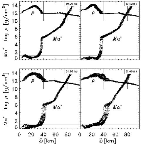
Figure 8: Scatter plots of the density (upper “curves”, logarithmic scale, in units of $[\mathrm{g\,cm}^{-3}]$) and the Mach number $M\!a^{*}$ (lower “curves”, calculated in a coordinate system rigidly rotating with the torus) in the equatorial plane $z\!=\!0$ versus distance $\varpi:=\sqrt{x^{2}+y^{2}}$ from the rotation axis at different instants in time (see upper right corner of each panel). The bold horizontal line separates supersonic (upper) from subsonic (lower) flow regions. The thin vertical lines indicate the boundaries $\xi_{\rm bound}$ of the nested grids (see text).

Our qualitative interpretation of this result is as follows: Non-axisymmetric instabilities have been shown to occur in MacLaurin spheroids as well as in a large variety of (differentially) rotating compressible fluid bodies in equilibrium, if the rate of rotation is sufficiently large. However, being equilibrium configurations, the instabilities in these models grow in the absence of any radial motion. When viewed from a suitably chosen rotating coordinate system sonic contact along the azimuthal coordinate is established in these models and allows for a coherent growth of the instability. According to our results, the latter condition seems to be sufficient for the growth of non-axisymmetric instabilities also in collapsing rotators. If on the other hand sonic contact is not given along the azimuthal coordinate due to large radial velocities — like in the outer core of our models — it is difficult to imagine how global tri-axial deformations can develop coherently. Thus, we suppose that sonic communication in azimuthal direction is also a necessary condition for the growth of non-axisymmetric instabilities.

One might argue that these results depend on our particular choice of the rotating coordinate system. However, establishing co-rotation at any distance $\varpi$ (i.e., chosing a coordinate system rotating with an angular velocity equal to that of the fluid at that distance) outside the domain of the inner torus does not allow to “transform away” supersonic velocities in the collapsing (outer) core, since the radial component dominates the angular component of the velocity field by a large amount.

3.4 Gravitational wave signal

Although models MD1 and MD2 show prominent deviations from axisymmetry, the gravitational wave signal is changed only marginally compared with the axisymmetric calculation. In particular, the maximum wave amplitudes are equal for the 3D and the 2D simulations within an accuracy of 2%. The waveforms and the energy radiated in form of gravitational waves are displayed in Fig. 9. The peak amplitude of $h_{+}$ is reached at about the time of bounce in both the 2D and the 3D models. Up to this point in the evolution the waveforms are identical, too. This is not surprising, since the initial perturbations of models MD1 and MD2 have not grown significantly until the time of bounce, which occurs only 0.5 ms after $\beta_{\rm dyn}$ is reached. As discussed above, the density contrast is $\delta\varrho\la 0.15$ inside the inner torus before bounce. Accordingly, $h_{\times}$, which is of genuine non-axisymmetric origin nearly vanishes until bounce (Fig. 9).

The maximum amplitudes of $h_{\times}$ are reached during the further evolution, when the spiral arms merge to form the final bar (model MD2) or when the transient $m=4$ structure evolves to some “bar-like” configuration (model MD1). These maxima are only of the order of 10% of the maximum value of $|h_{+}|$. The amplitudes of the cross- and plus-polarizations finally become comparable, because the inner core (torus) approaches its new rotational equilibrium and thus the time derivatives of the quadrupole moments due to radial motion become steadily smaller. The periodicity seen in $h_{\times}$ is due to a nearly solid-body type rotation of the high density regions of the core.

Figure 9: Gravitational wave amplitudes $rh_{+}(x\!=\!r,y\!=\!0,z\!=\!0)$, (thick lines), $rh_{\times}(x\!=\!0,y\!=\!0,z\!=\!r)$, (thin lines) and radiated energy $E_{\rm GW}$ as functions of time for the three-dimensional models MD1 (dashed) and MD2 (dashed-dotted) in comparison with the axisymmetric calculation (solid). The peak values $|rh|\simeq 1000$ cm correspond to dimensionless amplitudes $|h|\approx 3\,10^{-23}$ for a source at $r=10$ Mpc.

Comparing the 3D results with the 2D signal, one notices that the 3D waveforms do not reproduce the small additional local minimum in $h_{+}$ visible at $t\approx 31$ ms for the axisymmetric model. Also the (absolute values of the) time derivatives of $h_{+}$ are smaller for the following 2 ms. This leads to a smaller value of the amount of energy radiated in form of gravitational waves (Eq. 10; for model MD1 $h_{+}$ is roughly proportional to $\ddot{I}{{\scriptscriptstyle\stackrel{{\scriptstyle-}}{{}}}}_{xx}$ and $\ddot{I}{{\scriptscriptstyle\stackrel{{\scriptstyle-}}{{}}}}_{yy}$ during this time interval because of the near axisymmetry of the core at this time). We have analyzed carefully the unexpected fact that compared to the axisymmetric models we obtain only 65% of the gravitational wave energy for the two models MD1 and MD2, which during this epoch are approximately, but not exactly axisymmetric. Several tests and comparisons (e.g., with poorer resolved 2D calculations) have shown that this is not a possibly unnoticed 3D effect, but due to a somewhat lower “angular” resolution of the 3D simulation compared with the best resolved 2D run (see Rampp (1997) for details). The lower resolution gives rise to a larger violation of total energy conservation, most of which occurs during bounce. Since all dynamical quantities of model MD1 – local as well as global ones – agree with the 2D results within an accuracy of a few percent, we consider the observationally relevant waveforms calculated in the 3D simulations to be reliable within the underlying approximations (cf. sect. 2). We also point out the fact that the squared time derivatives of the moments $\ddot{I}{{\scriptscriptstyle\stackrel{{\scriptstyle-}}{{}}}}_{ij}$ enter the formula for the radiated energy. Small deviations in the waveforms therefore can account for quite large differences in the energies. It is not surprising, though not easy to explain in detail, that the 3D waveforms differ from the axisymmetric waveforms at later times $t\ga 33$ ms, when the dynamical evolution of these models is changed significantly due to their non-axisymmetric inner cores.

Given the dynamical evolution of the core, the small magnitude of the amplitudes $h_{\times}$ can easily be explained by utilizing the well known order-of-magnitude argument for the quadrupole waveforms

$$rh_{\times}\simeq 2\,\frac{G}{c^{4}}\frac{I{\scriptscriptstyle\stackrel{{\scriptstyle-}}{{}}}}{T^{2}}\simeq 2\,\frac{G}{c^{4}}\,\frac{0.1MR^{2}}{T^{2}}\simeq 100\mbox{\,cm}\,.$$ (21)

According to the results of our computations, we have inserted the quadrupole moment $I{\scriptscriptstyle\stackrel{{\scriptstyle-}}{{}}}$ of a homogeneous bar with mass $M\sim 0.5\,{M_{\odot}}$, length $R\sim 100$ km and rotation period $T\sim 5$ ms. Approximating the non-axisymmetrically distributed mass of $\sim 0.5\,{M_{\odot}}$ as two point masses orbiting each other at a distance of 100 km with an angular velocity equal to the observed one, yields the same order-of-magnitude for $h_{\times}$.

Finally, by using the quadrupole formulae (Eqns. 7 and 8) we may have underestimated the amount of gravitational radiation produced by model MD2, particularly during the phase when the $m=3$ symmetry of the inner core is most prominent. We estimate the order-of-magnitude of the mass-octupole contribution to the signal by (e.g., Blanchet et al. 1990, Eq. 6.8)

$$rh^{\rm TT}_{\rm oct}\simeq 2\frac{G}{c^{4}}\frac{3}{c}\frac{MR^{3}}{T^{3}}\simeq 3R_{\rm s}\left(\frac{v}{c}\right)^{3}\la 500\mbox{\,cm}\,,$$ (22)

where $v\sim 0.1\,c$ and $M\sim 0.5\,{M_{\odot}}$ and a Schwarzschild radius $R_{\rm s}\sim 1.5\,10^{5}$ cm was assumed. Hence, the mass-octupole radiation cannot account for significant enhancement of the peak amplitudes of our model MD2 compared with the axisymmetric case (Fig. 9) or MD1, although it might change the details of the waveforms.

Figure 10: Rotation parameter $\beta$ as a function of time for the three-dimensional model MD3 (dotted), which suffers a second collapse. For comparison the evolution of $\beta$ of model MD1 is shown, too (dashed).

3.5 Second collapse of a non-axisymmetric core

After bounce, the proto-neutron star settles into its new rotational equilibrium, and cools and contracts on a secular time scale, which is given by the neutrino-loss time scale ($\simeq 10$ s; see e.g., Keil & Janka 1995 and references cited therein). According to linear stability analysis tri-axial perturbations grow on this time scale, provided the rotation parameter $\beta\ga 0.14$. For numerical reasons (because our hydrodynamic code is explicit and thus the time step is limited by the CFL stability condition; see e.g., LeVeque 1992) as well as for physical reasons (neglect of weak interactions and neutrino transport) our approach is inadequate for simulating this secular evolution. However, we are able to consider a sudden reduction of the stabilizing pressure in a deformed, non-axisymmetric, rapidly rotating post-bounce core (model MD3). This extreme case cannot provide the answer to the question whether secular instabilities will indeed grow to nonlinear amplitudes and what their influence will be on the evolution of the core. Nevertheless, such a simulation can shed some light on the problem how much gravitational radiation can be expected, when a rapidly rotating non-axisymmetric neutron star forms.

Figure 11: Snapshots of the density distribution (in units of [$\mathrm{g\,cm}^{-3}$]) and the velocity field in the equatorial plane of model MD3. The contours are logarithmically spaced with intervals of 0.25 dex, they are shaded with darker grey values for higher density regions and labeled with their respective values. The time of the snapshot and the velocity scale are given in the upper right corner of each panel.

We choose model MD1 at $t=43.12$ ms as the starting point for the simulation (Fig. 11a). At this time we (suddenly) reduce $\Gamma_{1}$ from its original value of 1.28 to a value of 1.2. This renders the rotating core unstable against a second dynamic collapse. In passing we note that the stability criterion due to Ledoux (1945; Eq. 77) would require $\Gamma_{1}\la 1.18$ for a rigidly rotating core in equilibrium with $\beta\approx 0.16$ to collapse.

Figure 12: Gravitational wave amplitudes $rh_{+}(x\!=\!r,y\!=\!0,z\!=\!0)$, (thick lines) and $rh_{\times}(x\!=\!0,y\!=\!0,z\!=\!r)$, (thin lines) as functions of time for the three-dimensional model MD3 (dotted), where $r$ denotes the distance to the source. For comparison the amplitudes of model MD1 are shown, too (dashed).

The overall contraction, bounce and re-expansion of model MD3 is reflected in the time evolution of the rotation parameter $\beta$. Note, that concerning the development of non-axisymmetric instabilities the absolute value of $\beta$ is not very relevant here, because the initial “perturbations” are already in the non-linear regime. Compared to the (first) collapse of model MD1 we find a somewhat longer time scale for the contraction and re-expansion in model MD3. The peak value of $\beta\approx 0.23$ is considerably smaller than that of model MD1 ($\beta\approx 0.34$), because only mass shells with $M\la 0.5\,{M_{\odot}}$ contract to radii similar to those reached during the collapse of model MD1. Mass shells of model MD3 with $M\ga 0.8\,{M_{\odot}}$ remain nearly unaffected by the sudden pressure reduction at $t=43.12$ ms.

During the collapse of model MD3 several pronounced density maxima are formed. They are all located inside the torus reaching peak values of $\varrho=5.3\,10^{14}\mathrm{g\,cm}^{-3}$. The five initial clumps forming at the density maxima contain a mass of $\approx 0.1\,{M_{\odot}}$ each (Fig. 11b). During the further evolution their number decreases as they merge one after the other. Eventually, just two of them remain, which form a bar-like or binary-like deformed central region (Fig. 11c and d).

The maximum density on the grid (reached in the clumps) sharply rises from $2\,10^{13}\mathrm{g\,cm}^{-3}$ to $5.3\,10^{14}\mathrm{g\,cm}^{-3}$ within a fraction of a millisecond after pressure reduction. The collapse is, however, rapidly decelerated by the action of centrifugal forces, which also eventually cause a bounce at $t\approx 46$ ms (Fig. 10). The pressure increase resulting from matter whose density exceeds nuclear matter density is dynamically unimportant, as only a negligible amount of mass inside some of the clumps is involved (Fig. 11).

Model MD3 shows a highly non-axisymmetric, bar-like density stratification already before the (second) bounce occurs at $t\approx 46$ ms (Fig. 11b). This is different from the behaviour of models MD1 and MD2, where large non-axisymmetries (quadrupole moments) only appear well after bounce, i.e., after the most rapid phase of the evolution. Accordingly, one expects larger time derivatives of larger quadrupole moments and therefore a stronger gravitational wave signal from model MD3 than either from model MD1 or MD2.

The actual waveforms for model MD3 are shown in Fig. 12. Compared to model MD1 one notices a considerably larger value for the genuinely non-axisymmetric polarization amplitude $h_{\times}$. The maximum values $|rh_{\times}|\approx 800$ cm and $|rh_{+}|\approx 300$ cm do, however, neither exceed the peak value of $|rh_{+}|$ obtained in the axisymmetric simulation at bounce nor those of the three-dimensional models MD1 and MD2 (Fig. 12).

Additional (axisymmetric) simulations with $\Gamma_{1}$ reduced to 1.2 or 1.25 have shown that the peak value of $\beta$, the time scale of the (second) collapse as well as the peak values of the gravitational waveforms do not depend strongly on the exact value of $\Gamma_{1}$.

4 Summary and discussion

We have presented three-dimensional hydrodynamic simulations of the collapse of rapidly rotating stellar iron cores. The matter in the core has been described by a simple analytical equation of state. Effects due to neutrino transport have been neglected. Hydrodynamics and self-gravity has been treated in Newtonian approximation. The initial models for our simulations have been taken from the comprehensive parameter study of axisymmetric rotational core collapse performed by Zwerger & Müller (1997).

For our study we have selected those axisymmetric models which are secularly or dynamically unstable with respect to non-axisymmetric perturbations. Hence, in order to be selected the rotation rate parameter $\beta$ of a model had to exceed the critical rotation rates $\beta_{\rm sec}\approx 0.14$ or $\beta_{\rm dyn}\approx 0.27$ during its evolution. These critical rotation rates have been derived for incompressible MacLaurin spheroids, but also hold approximately for a wide range of compressible equilibrium configurations (e.g., Tassoul 1978). After mapping the rapidly rotating axisymmetric cores onto the three-dimensional computational grid, we imposed an initial non-axisymmetric perturbation and simulated the further evolution with a three-dimensional variant of the PROMETHEUS hydrodynamic code. The simulations cover a time interval from a few milliseconds before core bounce up to several tens of milliseconds after bounce.

We have used the quadrupole formula to calculate the gravitational wave signal and have estimated the contribution of the next-leading radiative-multipole order, which is negligibly small. Because of its smallness gravitational radiation reaction was not taken into account.

Our 3D simulations show that in two models, which are secularly but not dynamically unstable ($0.15\leq\beta\leq 0.2$) non-axisymmetric perturbations do not grow. Consistent with this result, we also observe no significant enhancement of the gravitational wave emission in these models compared to the axisymmetric case.

Among the models investigated by Zwerger & Müller (1997) there is only one model where $\beta>\beta_{\rm dyn}$ during the evolution. This is their most rapidly and most differentially rotating model evolved with the softest equation of state. This axisymmetric model was perturbed about 2 ms before bounce by imposing a random density distribution of 10% amplitude. Despite the random initial perturbation, $m=2$ and $m=4$ toroidal modes are found to dominate the early evolution of the model, because of the set of cubic grids used in the simulation. Therefore, a second simulation was performed, where an additional $m=3$ toroidal perturbation of 5% amplitude was imposed initially.

The gross features of the evolution are quite similar in the axisymmetric and non-axisymmetric simulations. In both cases the overall evolution is characterized by a rapid contraction, bounce and re-expansion of the inner core. In the 3D simulations we, in addition, observe the growth of the initial perturbations. Until several milliseconds (or dynamical time scales of the inner core) after bounce the density distribution resembles the symmetry of the initially dominating modes. Subsequently, the core evolves towards a bar-like shaped configuration. In none of the 3D models the gravitational wave amplitude exceeds the axisymmetric value of $|h|=3.5\,10^{-23}$ (for a source at 10 Mpc), three dimensional effects on the waveforms being only of the order of 10%. Even when the collapsed, bar-like, rapidly rotating inner core is forced into a second collapse (by artificially reducing its adiabatic index), we do not observe gravitational wave amplitudes significantly larger than $|h|\simeq 10^{-23}$ (for a source at 10 Mpc).

In order to judge the implications of our results for rotational core collapse in general and for gravitational wave astronomy in particular, the following possible limitations of our approach should be kept in mind:

• Since $GM/Rc^{2}\la 0.2$ for the axisymmetric models of Zwerger & Müller (1997), general relativistic effects can be viewed as moderate corrections to Newtonian gravity as far as the collapse dynamics is concerned. However, since general relativity counteracts the stabilizing influence of rotation on radial modes (e.g., Tassoul 1978), its influence on the stability properties of (even only moderately compact) rotating iron cores can be of considerable importance. When GR is taken into account, pre-collapse models with a larger amount of angular momentum (and the same EOS) than in the Newtonian approximation can collapse. Furthermore, GR models will maintain higher densities as well as larger rotation parameters for a longer time interval after bounce as compared to Newtonian models (see the discussion in Zwerger & Müller 1997).

• The secular evolution (i.e., the evolution on time scales of hundreds of milliseconds) of the collapsed core is not known even in the axisymmetric case. Simulating this evolution requires models with detailed microphysics and thermodynamics, and an adequate treatment of the neutrino transport. However, even in 2D such simulations are still prohibitively time consuming. Thus, there might exist additional initial models different from those presently available, which could become unstable to tri-axial perturbations on a secular time scale (see however the next point).

• Concerning the limited set of axisymmetric initial models, we adopt the arguments given in Zwerger & Müller (1997). They claim that the large parameter space considered in their study most probably comprises the whole domain where actual pre-collapse rotating iron cores are to be found. They further argue that using a realistic equation of state instead of a polytropic one will change the details of the evolution, but will not give rise to qualitatively different results. In particular, it is unlikely that there exists a much larger set of pre-collapse initial models, which fulfill $\beta>\beta_{\rm dyn}$ and which are sufficiently compact for an extended time interval after core bounce.

  But even if there are models which fulfill these conditions and become triaxial, we do not expect them to produce a considerably stronger gravitational wave signal than the “best” axisymmetric models. Provided the initial amount of angular momentum is not unreasonably large, the critical rotation rates for non-axisymmetric instabilities can only be exceeded in collapsing cores with relatively soft equations of state (Eriguchi & Müller 1985, Zwerger & Müller 1997). But these soft equations of state drastically reduce both the mass and the radius of the inner core (Zwerger & Müller 1997). However, according to our 3D calculations, it is only in the inner core, where non-axisymmetric perturbations can grow significantly. Ta-ken together these considerations suggest that bar-like inner cores have masses less than $0.5\,{M_{\odot}}$, radii less than $100$ km, and rotation periods greater than $1$ ms. This implies a maximum gravitational wave amplitude $|h|\la 10^{-22}$ (for a source at 10 Mpc).

Given the most recent rates of core collapse supernova events (e.g., Cappellaro et al. 1997), which not all may involve a rapidly rotating core, we conclude that it is rather unlikely to expect gravitational wave signals from dynamic non-axisymmetric instabilities with sufficient strength and rate (i.e., several per year) to be observable with the large interferometric gravitational wave antennas presently under construction.

Movies in MPEG format of the dynamical evolution of all models are available in the world-wide-web at http: //
www.mpa-garching.mpg.de/~mjr/GRAV/grav3.html

- (1) Abramovici A. et al. , 1992, Science 256, 325
- (2) Aksenov A.G., 1996, Astronomy Letters 22, 634
- (3) Blanchet L., Damour T., Schäfer G., 1990, MNRAS 242, 289
- (4) Bonazzola S., Marck J.-A., 1993, A&A 267, 623
- (5) Bonazzola S., Marck J.-A., 1994, Ann. Rev. Nucl. Part. Sci 45, 655
- (6) Bonnell I.A., Pringle J.E., 1995, MNRAS 273, L12
- (7) Cappellaro E., Turatto M., Tsvetkov D. Yu., Bartunov O. S., Pollas C., Evans R., Hamuy M. , 1997, A&A 322, 431
- (8) Chandrasekhar S. 1969, Ellipsoidal Figures of Equilibrium, Yale Univ. Press, New Haven
- (9) Chandrasekhar S. 1970, ApJ 161, 561
- (10) Chandrasekhar S., Lebovitz N., 1963, ApJ 137, 1162
- (11) Colella P., Woodward P.R., 1984, JCP 54, 174
- (12) Eriguchi Y., Müller E., 1985, A&A 147, 161
- (13) Finn L.S., Evans C.R., 1990, ApJ 351, 588
- (14) Fryxell B.A., Müller E., Arnett D., 1989, Max-Planck-Institut für Astrophysik Report 449, Garching, Germany
- (15) Goldreich P., Weber S.V., 1980, ApJ 238, 991
- (16) Houser J.L., Centrella J.M., Smith S.C., 1994, Phys. Rev. Lett. 72, 1314
- (17) Houser J.L., Centrella J.M., 1996, Phys.Rev. D54, 7278
- (18) Imamura J.N., Toman J., Durisen R.H., Pickett B.K., Yang S., 1995, ApJ 444, 363
- (19) Janka H.-Th., Zwerger T., Mönchmeyer R., 1993, A&A 268, 360
- (20) Keil W., Janka H.-Th., 1995, A&A 296, 145
- (21) Lai D., Shapiro S.L., 1995, ApJ 442, 259
- (22) Ledoux P., 1945, ApJ 102, 143
- (23) LeVeque R.J., 1992, Numerical methods for conservation laws (2nd ed), Lectures in mathematics - ETH Zürich, Birkhäuser, Basel
- (24) Lindblom L., Detweiler S.L., 1977, ApJ 211, 565
- (25) Marck J.-A., Bonazzola S., 1992, in Approaches to Numerical relativity, ed. R. D’Inverno, Cambridge Univ. Press, Cambridge, 247
- (26) Misner C.W., Thorne K.S., Wheeler J.A., 1973, Gravitation, Freeman, San Francisco
- (27) Mönchmeyer R., 1993, Ph.D. thesis, Technische Univ. München, 1993, unpublished.
- (28) Mönchmeyer R., Schäfer G., Müller E., Kates R., 1991, A&A 246, 417
- (29) Müller E., 1982, A&A 114, 53
- (30) Müller E., Hillebrandt W., 1981, A&A 103, 358
- (31) Nakamura T., Oohara K., 1989, in Frontiers in Numerical Relativity, eds. C.R. Evans, L.S. Finn, and D.W. Hobill, Cambridge Univ. Press, 254
- (32) Pickett B.K., Durisen R.H., Davis G.A, 1996, ApJ 458, 714
- (33) Piran T., 1990, in Supernovae, eds. J.C. Wheeler, T. Piran and S. Weinberg, World Scientific, Singapore, 303
- (34) Rampp M., 1997, Diploma thesis, Technische Univ. München, unpublished
- (35) Roberts P.H., Stewartson K., 1963, ApJ 137, 777
- (36) Ruffert M., 1992, A&A 265, 82
- (37) Schutz B.F., 1983, Lectures in Applied Mathematics 20, AMS, p. 97
- (38) Schutz B.F., 1989, Classical Quantum Gravity 6, 1761
- (39) Shapiro S.L., Lightman A.P., 1976, ApJ 207, 263
- (40) Smith S.C., Houser J.L., Centrella J.M., 1996, ApJ 458, 236
- (41) Tassoul J.-L., 1978, Theory of Rotating Stars, Princeton Univ. Press, New Jersey
- (42) Thorne K.S., 1980, Rev. Mod. Phys 52, 299
- (43) Thorne K.S., 1987, in Three Hundred Years of Gravitation, eds. S.W. Hawking and W. Israel, Cambridge University Press, Cambridge, pp.330
- (44) Thorne K.S.: 1995, Particle and Nuclear Astrophysics and Cosmology in the next Millenium, In: Proc. of the 1994 Snowmass Summer Study, E.W. Kolb and R.D. Peccei (eds.), World Scientific, Singapore, 160
- (45) Tohline J.E., 1984, ApJ 285, 721
- (46) Yahil A., 1983, ApJ 265, 1047
- (47) Yamada S., Sato K., 1994, ApJ 434, 268
- (48) Yamada S., Sato K., 1995, ApJ 450, 245
- (49) Zhuge X., Centrella J.M., McMillan L.W., 1994, Phys. Rev. D 50, 6247
- (50) Zwerger T., 1995, Ph.D. Thesis, Technische Univ. München, unpublished
- (51) Zwerger T., Müller E., 1997, A&A 320, 209