A detailed study of defect models for cosmic structure formation

Abstract

We calculate predictions from wide class of ‘active’ models of cosmic structure formation which allows us to scan the space of possible defect models. We calculate the linear cold dark matter power spectrum and Cosmic Microwave Background (CMB) anisotropies over all observable scales using a full linear Einstein-Boltzmann code. Our main result, which has already been reported, points to a serious problem reconciling the observed amplitude of the large-scale galaxy distribution with the COBE normalization. Here, we describe our methods and results in detail. The problem is present for a wide range of defect parameters, which can be used to represent potential differences among defect models, as well as possible systematic numerical errors. We explicitly examine the impact of varying the defect model parameters and we show how the results substantiate these conclusions. The standard scaling defect models are in serious conflict with the current data, and we show how attempts to resolve the problem by considering non-scaling defects or modified stress-energy components would require radical departures from what has become the standard picture.

I Introduction

Topological defects are an almost generic phenomena in nature and have been already detected in a number of laboratory systems (see, for example, ref.[1]), where symmetry breaking phase transitions take place. Probably the most exciting possibility, however, is that they are formed during spontaneous symmetry breaking at a phase transition in the early universe [2, 3, 4], since they could act as the primordial seeds for galaxy formation; the most plausible models being the so called cosmic string [5, 6] and cosmic texture [7] theories.

Theories for galaxy formation can be described as either ‘passive’ or ‘active’ [8]. In passive theories, such as those predicted by the inflationary paradigm, all the perturbations are set up effectively as (super-horizon) initial conditions at very early times, which then evolve under a deterministic linear evolution, until very late when non-linear processes take over on the very smallest scales. By contrast, perturbations are created on all scales at all times in active models making predictions much more difficult to calculate. Typically, one has to deal with the fundamental non-linearity of the source over a large dynamic range — approximately 25 orders of magnitude — from the defect formation to the present.

The last few months have seen dramatic progress in pinning down the predictions from defect models of cosmic structure formation in what we shall describe as the standard scenario, that is defect motivated stress-energy components with an assumption of perfect scaling from formation to the present day. Three groups[9, 10, 11] have performed calculations which integrate the linear Einstein-Boltzmann equations using the latest technology for different models of the defect stress-energy two-point functions to produce predictions of power spectra for the cold dark matter (CDM) density field and the Cosmic Microwave Background (CMB) anisotropies. This article gives a detailed presentation of the methods and results of ref. [10].

There are two traditional approaches to the study of defect dynamics. Some authors have used large-scale simulations to provide the sources for their CMB and structure formation calculations [12, 13, 14, 15], while others have developed analytic models which attempt to describe the statistical properties of the defects [16, 17, 18]. Even using the latest technology, modelling the source using simulations is severely constrained by dynamic range. In this work, we will use a model based approach to calculate the two-point correlation functions, which act as sources for a state-of-the-art linear Einstein-Boltzmann solver. This has a number of advantages and also disadvantages when compared with the complementary simulation based approach; the real strength being that one is not constrained to a particular defect based scenario, allowing one to explore all possible scenarios and understand the robustness of any claims that one might make. The downside is that one must take care to construct the source stress-energy, which has many possible degrees of freedom, in a way which is at least physically plausible. This is generally done by comparison to some kind of simulation.

The recent work by Pen et al [9] and our collaboration [10], has exposed an apparently deep conflict between COBE normalized defect models and the observed galaxy correlations on large scales. The conflict was quantified in ref.[10] in terms of $b_{100}$, the bias between the dark matter and baryon distributions on scales of $100h^{-1}$Mpc required to match the COBE normalized defect models with the galaxy data. Although some evidence for such a problem has existed for some time, uncertainties about whether the computations had sufficient dynamic range meant the precise quantitative details of the problem were not fully understood. Most previous work on this problem relied on separate calculations for the large-angle CMB, which is normalized to COBE, and the linear matter power spectrum, using analytic expressions to relate the two, via, for example, the mass per unit length in the case of cosmic strings. Our calculations (as well as those of Pen et al [9]) do not use any such extrapolation, with the perturbations in the matter (dark and baryonic) and the photon (plus neutrinos) distributions being calculated in a self consistent way across all observable scales. Hence, a single normalization to COBE gives the normalized linear matter power spectrum.

We should note that the scale of $100h^{-1}$Mpc was chosen for three reasons. Firstly, $100h^{-1}$Mpc is sufficiently large that non-linear effects are not expected to affect the power spectrum. Secondly, the discrepancy in the power spectra at this scale is at its most extreme. And finally, it is unlikely that the power spectrum on these scales can be affected by changes in the cosmogony, for example, the introduction of hot dark matter (HDM).

The price of our solution to the dynamic range problem is that (1) we can only calculate the power spectrum of the matter and CMB since we have only included the two-point functions of the source [19] — no non-Gaussian effects are included — and (2) the results depend on the validity of the simple scaling picture over many orders of magnitude of cosmic expansion. Even though there is substantial support for this assumption, both from numerical simulations and analytic modelling[20, 21, 22, 16, 17, 18], there are also reasons to think that it may not be perfect. One of the important components of our work is an investigation of possible deviations from scaling. Our approach to modelling the defect two-point functions has also allowed us to explore other variations, besides deviations from scaling. These variations represent possible differences between defect models and possible systematic errors in numerical defect simulations. We have found that solving the $b_{100}$ problem requires extreme departures from the standard picture. (Interestingly, we are learning that defect networks in $\Omega_{matter}<1$ cosmologies may exhibit interesting levels non-scaling behaviour[23, 24].)

In the next section, we discuss some aspects of the linearized Einstein-Boltzmann solver, in particular the inclusion of source stress-energy, the Einstein-Boltzmann equations for vector perturbations and ways of calculating the ensemble average for incoherent perturbations. Section III presents in detail our modelling of the source two-point functions, by reference to a specific string motivated model. The results for the standard scaling model are presented along with quantification of the $b_{100}$ problem. We also show that simple modifications to the model and cosmological parameters, such as the Hubble constant and baryon density, have little impact on the $b_{100}$ problem. In Section IV we discuss possible deviations from the standard scaling assumption and section V explores further modifications to the model, which might lead to an improvement in the comparison with the data. We find that it is possible to get better agreement, although only the most extreme modifications come close on $100h^{-1}$Mpc scales. The aim of this paper is to present a pedagogical exposition of our work, so that the expert can reproduce and interpret our results. In the final section, we discuss its relation to that of others and point to directions of future investigation.

II Linear Einstein-Boltzmann solver

A CMBFAST

In order to calculate CMB anisotropies, one must solve the linearized Einstein-Boltzmann equations. Recent years have seen techniques developed to solve these equations to very high precision $(\sim 1\%)$ for the standard adiabatic models based on inflation [26], culminating in the public release of CMBFAST [28] which can perform this task in under a minute on a modern workstation. The standard Boltzmann method involves evolving over 3000 highly oscillatory linear ODEs from some time deep in the radiation era to the present day, which can take many hours. The line of sight method [25] used in this code reduces the time drastically by splitting the prohibitively oscillatory geometric effects from the dynamical processes due to, for example, the Doppler effect and potential evolution. This reduces the number of ODEs down to about 30, but adds an integration along the line of sight.

It is usual to express temperature anisotropies in terms of a decomposition into spherical harmonics,

$${\Delta T\over T}(\theta,\phi)=\sum_{l=0}^{\infty}\sum_{m=-l}^{l}a_{lm}Y_{lm}(\theta,\phi)\,.$$ (1)

For a Gaussian random field, such as those generated by inflation, the statistics of anisotropies are entirely specified by the angular power spectrum $C_{l}=\langle|a^{2}_{lm}|\rangle$ where the angled brackets denote an ensemble average.

For the moment, let us assume that we only require the anisotropies for a simple inflationary model which creates no appreciable vector and tensor fluctuations. In this case, the angular power spectrum is given by

$$C_{l}={2\over\pi}\int k^{2}dk\langle\Delta^{S}_{l}(k,\tau_{0})\Delta^{S*}_{l}(k,\tau_{0})\rangle\,,$$ (2)

where the photon distribution function $\Delta^{S}_{l}(k,\tau_{0})$ at the present day $\tau=\tau_{0}$ is given by the line of sight integration,

$$\Delta^{S}_{l}(k,\tau_{0})=\int_{0}^{\tau_{0}}d\tau\left(S^{0}_{T}(k,\tau)j^{00}_{l}\left[k(\tau_{0}-\tau)\right]+S^{1}_{T}(k,\tau)j^{10}_{l}\left[k(\tau_{0}-\tau)\right]+S^{2}_{T}(k,\tau)j^{20}_{l}\left[k(\tau_{0}-\tau)\right]\right)\,,$$ (3)

and $S^{0}_{T}(k,\tau)$, $S^{1}_{T}(k,\tau)$, $S^{2}_{T}(k,\tau)$ can be deduced from ref.[27], with

$$j^{00}_{l}(x)=j_{l}(x)\,,\quad j^{10}(x)=j^{\prime}_{l}(x)\,,\quad j^{20}_{l}(x)={1\over 2}\left(3j_{l}^{\prime}(x)+j_{l}(x)\right)\,.$$ (4)

For the coherent limit, implicit in phase focused [8] inflationary models, one can perform the ensemble average by simply replacing $\langle\Delta^{S}_{l}(k,\tau_{0})\Delta^{S*}_{l}(k,\tau_{0})\rangle=|\Delta^{S}_{l}(k,\tau_{0})|^{2}$.

In the rest of this section, we will describe how this approach can be modified to include active sources such as cosmic defects. Firstly, we show how simple coherent scalar sources may be added. Then we discuss the inclusion of the vector and tensor sources, almost generic in any active model. Finally, we show how one may perform the ensemble average when the source is not coherent and discuss the various implications of decoherence. We have already noted that for non-Gaussian sources, such as the topological defects under consideration here, the angular power spectrum does not entirely specify the nature of the of anisotropies. However, most realistic models are thought to lead to only mildly non-Gaussian anisotropies through the Central Limit Theorem for the superposition of non-Gaussian probability distributions. Hence, it should be a useful discriminant between different models for structure formation. We will discuss the efficacy of using power spectra to distinguish between different models of structure formation in the conclusions.

B Coherent active scalar sources

As a first step, therefore, let us introduce an independent covariantly conserved component of stress-energy $\Theta_{\mu\nu}$ into the Einstein equations,

$$G_{\mu\nu}=8\pi\left[T_{\mu\nu}+\Theta_{\mu\nu}\right]\,,$$ (5)

where $T_{\mu\nu}$ is the stress-energy of CDM, baryons, photons and neutrinos present in a particular cosmogony. This extra component, usually assumed to be ‘stiff’, that is, unaffected by gravity at first order, adds a forcing term to the Einstein-Boltzmann equations which represents the active sources.

For the moment let us assume that the Fourier transform of the stress-energy can be decomposed as $\Theta_{0i}=\Theta_{D}\hat{k}_{i}$ and

$$\Theta_{ij}={1\over 3}\delta_{ij}\Theta+\left(\hat{k}_{i}\hat{k}_{j}-{1\over 3}\delta_{ij}\right)\Theta^{S}\,,$$ (6)

where $\hat{k}_{i}$ is a unit vector in Fourier space, $\Theta_{D}$ is the velocity field, $\Theta$ is the isotropic pressure, or three times the pressure, and $\Theta^{S}$ is the anisotropic stress. The conservation equations for this decomposition are

$$\dot{\Theta}_{00}+{\dot{a}\over a}\left(\Theta_{00}+\Theta\right)-\Theta_{D}=0\,,$$ (7)

$$\dot{\Theta}_{D}+{2\dot{a}\over a}\Theta_{D}+{1\over 3}k^{2}\left(\Theta+2\Theta^{S}\right)=0\,.$$ (8)

Hence, in order to incorporate this source stress-energy, one must add (8) to the ODE solver, modify the linearized Einstein equations to include the forcing terms and specify two quantities from $\Theta_{00}$, $\Theta_{D}$, $\Theta$ and $\Theta^{S}$.

The initial conditions for the Einstein-Boltzmann equations must also be modified. The idea is that one sets up initial conditions for a pure growing mode deep in the radiation era. In order to enforce causality, one requires that components of the pseudo-stress-energy tensor $\tau_{\mu\nu}$ be zero[12], which creates a balance between the initial metric perturbations, the defect stress-energy and the matter perturbations. However, there is a residual degree of freedom which allows us to just simply set everything to zero. Physically, this implies that the initial conditions are unimportant relative to the actual sources themselves, which is implicit in the distinction between passive and active sources.

The most common defect based models are thought to scale for most of the history of the universe and so for the moment at least, we specialize our discussion to scaling sources. This requires that $\tau^{1/2}\Theta_{00}(k,\tau)=F_{1}(k\tau)$, $\tau^{1/2}\Theta(k,\tau)=F_{2}(k\tau)$, $\tau^{1/2}\Theta_{D}(k,\tau)=F_{3}(k\tau)$ and $\tau^{1/2}\Theta^{S}(k,\tau)=F_{4}(k\tau)$, with the functions $F_{i}(x)$ having well defined power series expansions around $x=0$. Moreover, further constraints can be placed on the leading order behaviour of these functions by causality and analyticity [29]. In particular, this implies that,

$$\langle\Theta_{00}\Theta^{*}_{00}\rangle=Zk^{0}+{\cal O}(k^{2})\,,\quad\langle\Theta^{S}\Theta^{S*}\rangle=Yk^{0}+{\cal O}(k^{2})\,,\quad\langle\Theta_{00}\Theta^{S*}\rangle=Xk^{2}+{\cal O}(k^{4})\,,$$ (9)

$$\langle\Theta\Theta^{*}\rangle=Wk^{0}+{\cal O}(k^{2})\,,\quad\langle\Theta_{D}\Theta^{*}_{D}\rangle=Vk^{4}+{\cal O}(k^{6})\,,$$ (10)

with all the other correlators and cross-correlators being deduced in a similar way or by assuming stress-energy conservation. In the coherent limit $\langle\Theta_{00}\Theta^{S*}\rangle=\langle\Theta_{00}\Theta^{*}_{00}\rangle^{1/2}\langle\Theta^{S}\Theta^{S*}\rangle^{1/2}$, which using (10) implies that $Y=0$ and in fact $\langle\Theta^{S}\Theta^{S*}\rangle\sim k^{4}$. This very specialized limit leads to some slight subtleties which will not in general be present for active sources. This will be discussed in the section on incoherent sources.

One simple choice which is consistent with the coherent limit is to define [30]

$$4\pi\Theta={3\alpha\over\tau^{1/2}}{\sin Ak\tau\over Ak\tau}\,,\quad 4\pi\Theta^{S}={\beta\over\tau^{1/2}}{6\over B^{2}-C^{2}}\left({\sin Bk\tau\over Bk\tau}-{\sin Ck\tau\over Ck\tau}\right)\,,$$ (11)

where $A$, $B$, $C$, $\alpha$ and $\beta$ are constants. The angular power spectra for this source are presented in Fig. 1 for (a) $\alpha=1$, $\beta=0$ and $A=1$ (b) $\alpha=1$, $\beta=1$, $A=1$, $B=1$ and $C=0.5$. Taking into account the arbitrary normalization used in ref.[30], the results seem to be identical.

FIG. 1.: The angular power spectrum for the simple coherent sources (a,solid line) and (b,dotted line) normalized to COBE. Note no vector or tensor components are calculated here.

At a very technical level, various modifications to internal systems parameters of CMBFAST were also required. The source function for $\Delta^{S}_{l}(k,\tau)$ is dependent on three variables and the code sets up a discrete three-dimensional array containing these values with spacings $\Delta l$, $\Delta k$ and $\Delta\tau$, before performing the line of sight integration over $l$ values. Obviously, the most accurate results are obtained by using the smallest possible values of $\Delta l$, $\Delta k$ and $\Delta\tau$; the cost being an increase in the CPU time. We systematically reduced all three spacings from the values in the original version and found that the results converged when $\Delta k$ was reduced by about a factor of two, with $\Delta l$ and $\Delta\tau$ being left the same. We also varied the number of equations solved by the ODE integrator and found that there was no discernible improvement from any increase. We concluded that the line of sight integration method is also useful to calculate the predictions of active models for structure formation.

C Generalization to include vector and tensor modes

The split of the energy momentum tensor (6) is not the most general since it includes only scalar sources. A more general split is

$$\Theta_{0i}=\Theta_{D}\hat{k}_{i}+\Theta_{0i}^{V}\,,\quad\Theta_{ij}={1\over 3}\delta_{ij}\Theta+\left(\hat{k}_{i}\hat{k}_{j}-{1\over 3}\delta_{ij}\right)\Theta^{S}+\left(\hat{k}_{i}\Theta^{V}_{j}+\hat{k}_{j}\Theta^{V}_{i}\right)+\Theta_{ij}^{T}\,,$$ (12)

which includes vector $(\Theta_{0i}^{V},\Theta^{V}_{i})$ and tensor $(\Theta_{ij}^{T})$ sources such that

$$\hat{k}_{i}\Theta_{0i}^{V}=\hat{k}_{i}\Theta^{V}_{i}=\hat{k}_{i}\Theta^{T}_{ij}=\hat{k}_{j}\Theta^{T}_{ij}=\Theta^{T}_{ii}=0\,.$$ (13)

Without loss of generality, one can fix the direction in Fourier space and choosing $\hat{k}=(0,0,1)$ gives

$$\Theta_{\mu\nu}=\left(\begin{array}[]{cccc}\Theta_{00}&\Theta_{01}^{V}&\Theta_{02}^{V}&\Theta_{D}\\ \Theta_{01}^{V}&{1\over 3}\Theta-{1\over 3}\Theta^{S}+\Theta_{11}^{T}&\Theta_{21}^{T}&\Theta_{1}^{V}\\ \Theta_{02}^{V}&\Theta_{21}^{T}&{1\over 3}\Theta-{1\over 3}\Theta^{S}-\Theta_{11}^{T}&\Theta_{2}^{V}\\ \Theta_{D}&\Theta_{1}^{V}&\Theta_{2}^{V}&{1\over 3}\Theta+{2\over 3}\Theta^{S}\end{array}\right)\,,$$ (14)

with $\Theta_{03}^{V}=\Theta_{3}^{V}=\Theta_{3i}^{T}=\Theta_{i3}^{T}=0$ for $i=1,2,3$ and $\Theta^{T}_{11}+\Theta^{T}_{22}=0$. There appear to be four independent vector components $(\Theta_{1}^{V},\Theta_{2}^{V},\Theta_{01}^{V},\Theta_{02}^{V})$ and two tensor components $(\Theta_{11}^{T},\Theta_{21}^{T})$. However, two of the vector components are related to the other two by stress-energy conservation, and hence there are also just two independent components.

These vector and tensor sources can be identified with their respective contributions to the angular power spectrum $C_{l}=C_{l}^{S}+C_{l}^{V}+C_{l}^{T}$ which are defined in analogy to (2) by

$$C_{l}^{I}={2\over\pi}\int k^{2}dk\langle\Delta^{I}_{l}(k,\tau_{0})\Delta^{I*}_{l}(k,\tau_{0})\rangle\,,$$ (15)

where the index $I$ runs over $I=S,V,T$ corresponding to the scalar, vector, tensor contributions. The scalar photon distribution function is given in (3), with the vector and tensor versions defined by

$$\Delta^{V}_{l}(k,\tau_{0})=\displaystyle{\int_{0}^{\tau_{0}}d\tau\left(V^{1}_{T}(k,\tau)j^{11}_{l}\left[k(\tau_{0}-\tau)\right]+V^{2}_{T}(k,\tau)j^{21}_{l}\left[k(\tau_{0}-\tau)\right]\right)}\,,$$ (16)

$$\Delta^{T}_{l}(k,\tau_{0})=\displaystyle{\int_{0}^{\tau_{0}}d\tau\left(T^{2}_{T}(k,\tau)j^{22}\left[k(\tau_{0}-\tau)\right]\right)}\,,$$ (17)

where $V^{1}_{T}$, $V^{2}_{T}$, $T^{2}_{T}$ are the source functions for the vector and tensor perturbations and

$$j_{l}^{11}(x)=\sqrt{l(l+1)\over 2}{j_{l}(x)\over x}\,,\quad j_{l}^{21}(x)=\sqrt{3l(l+1)\over 2}\left({j_{l}(x)\over x}\right)^{\prime}\,,\quad j_{l}^{22}(x)=\sqrt{{3\over 8}{(l+2)!\over(l-2)!}}{j_{l}(x)\over x^{2}}\,.$$ (18)

The Boltzmann equations for the scalar and tensor perturbations are well studied both analytically and numerically, but the same is not true for vector perturbations. Here, we include the Boltzmann equations for the vector perturbations, along with a discussion of their salient features. For a more in depth study of scalar, vector and tensor perturbations, the reader is referred to ref.[27] which also includes all the other relevant Boltzmann equations.

We split up the photon distribution function for the vector sources into its angular multipole moments

$$\Delta^{V}(k,\tau_{0},\mu)=\sum_{l=1}^{\infty}(-i)^{l}(2l+1)P_{l}(\mu)\Delta^{V}_{l}(k,\tau_{0})\,,$$ (19)

where $\mu=\cos\theta$ is the angular variable. With this decomposition the Boltzmann equations become

$$\dot{\Delta}_{l}^{V}=k\left({\sqrt{l^{2}-1}\over 2l+1}\Delta^{V}_{l-1}-{\sqrt{l^{2}+2l}\over 2l+1}\Delta^{V}_{l+1}\right)-\dot{\kappa}\Delta^{V}_{l}+S_{l}$$ (20)

for $l>0$, where $\dot{\kappa}$ is the differential cross-section due to Thomson scattering,

$$S_{1}={1\over 3}\dot{\kappa}\left(V_{B}+\dot{V}\right)\,,\quad S_{2}={1\over 5}P^{V}={1\over 10}\dot{\kappa}\left(\Delta^{V}_{2}-\sqrt{6}E^{V}_{2}\right)\,,$$ (21)

and $S_{l}=0$ for $l>2$. In the above expression, $E^{V}_{2}$ is the quadrapole of the electric component of the photon polarization distribution and $V$ is the vector metric perturbation which satisfies

$$\dot{V}+{2\dot{a}\over a}V=-{64\pi G\over 25\sqrt{3}k}\left(\rho_{\gamma}\Delta^{V}_{2}+\rho_{\nu}N^{V}_{2}\right)-{8\pi G\over k}\Theta^{V}\,,$$ (22)

where $\Theta^{V}$ is the vector source, either $\Theta^{V}_{1}$ or $\Theta^{V}_{2}$, $\rho_{\gamma}$ is the average photon density, $\rho_{\nu}$ is equivalent quantity for neutrinos and $N^{V}_{2}$ is the quadrupole component of the neutrino distribution. $V_{B}$ is the vector (vortical) component of the baryon velocity which satisfies

$$\dot{V}_{B}=\dot{V}-{\dot{a}\over a}\left(V_{B}-V\right)+{\dot{\kappa}\over R}\left(3\Delta^{V}_{1}-V_{B}\right)\,,$$ (23)

where $R=3\rho_{b}/4\rho_{\gamma}$ and $\rho_{b}$ is the average baryon density. As already discussed the standard approach is to solve these linear differential equations equations for $l<l_{\rm max}$, plus the equivalent equations for the polarization distribution functions, which we have not included here for brevity. The line of sight integration method which we use only requires $l_{\rm max}\approx 7$, hence reducing the amount of CPU time required. However, we need one final ingredient, the source functions for vector perturbations, which are given by

$$V^{1}_{T}=\dot{\kappa}e^{-\kappa}\left(V_{B}-V\right)\,,$$ (24)

$$V^{2}_{T}=\dot{\kappa}e^{-\kappa}P^{V}+{1\over\sqrt{3}}e^{-\kappa}kV\,,$$ (25)

where

$$\kappa(\tau)=\int_{\tau}^{\tau_{0}}\dot{\kappa}(\tau^{\prime})d\tau^{\prime}\,,$$ (26)

is the optical depth due to Thomson scattering. We should note that exactly analogous expressions exist for both the electric and magnetic components of the polarization. These are also presented in ref.[27].

The important thing to notice is that vector perturbations are not created at any significant level in the absence of a source. This can be seen from the Einstein equation: if $\Theta_{V}=0$ then $V\propto a^{-2}$ since the effects of $\Delta^{V}_{2}$ and $N^{V}_{2}$ are negligible. Hence, they are not present in inflationary models, but are generic in any active model.

D Incoherent sources

In the previous few sections we have studied how the linearized Einstein-Boltzmann equations can be modified to include active sources which create scalar, vector and tensor anisotropies and we have shown how it is possible to relate to the measured quantities, such as the angular power spectrum, when the sources are coherent. Such sources are, however, very unnatural, generically relying on assumptions such as pure spherical symmetry to maintain coherence. Therefore, we are forced to consider methods for calculating the ensemble average for theories which include incoherent sources.

This subject was studied in a series of works which first discussed the equally unnatural, but probably more realistic, totally incoherent limit [8, 31] and then multi-parameter models which allowed for a gradual relaxation from total coherence to total decoherence [32]. One key advantage that the current work has over, for example, ref.[32] is that once a given source model is chosen there is no uncertainty in relative normalization of the anisotropy created by acoustic oscillations at the time of last scattering and that created much later by the ISW effect. The methods used in the earlier work suffered from large uncertainties in this aspect of the calculation. We shall see that decoherence is actually prevalent in most active models and the contribution to the anisotropy from the surface of last scattering does not, in general, give rise to noticeable acoustic type signatures in the angular power spectrum. We also find a suppression of the anisotropy created at last scattering with respect to the ISW effect, not anticipated in refs.[8, 31, 32].

The main problem in dealing with decoherence is that the unequal time correlators (UETC) do not factorize, that is,

$$\langle P(k,\tau_{1})P^{*}(k,\tau_{2})\rangle\neq\langle P(k,\tau_{1})P^{*}(k,\tau_{1})\rangle^{1/2}\langle P(k,\tau_{2})P^{*}(k,\tau_{2})\rangle^{1/2}\,,$$ (27)

for some arbitrary quantity $P(k,\tau)$ and $\tau_{1}\neq\tau_{2}$. There are two methods which one can use to overcome this problem. The first [33, 34], used in ref.[9], is to treat the UETC, evaluated at the discrete times used in the linear Einstein-Boltzmann solver, as a matrix which is symmetric and hence diagonalizable. This diagonalization yields a change of basis and the source can then be written as a sum of coherent sources,

$$\langle P(k,\tau_{1})P^{*}(k,\tau_{2})\rangle=\sum_{i}\lambda_{i}v_{i}(k,\tau_{1})v^{*}_{i}(k,\tau_{2})\,,$$ (28)

where the $\lambda_{i}$ are the eigenvectors, ordered such that $\lambda_{1}>\lambda_{2}>..>\lambda_{n}$, and $v_{i}(k,\tau)$ are the orthogonal, coherent basis functions. Since everything is linear, one can use each of these basis functions, as a source in the modified version of CMBFAST and the sum of the individual angular power spectra yields the total. Although each of these coherent sources is has a degree of acausality, it appears to give good convergence from using only the ten largest eigenvalues [9], which indicates that the full calculation is well behaved.

The second method [8], which is used in ref.[10] and the current work, is to not work directly with the UETC. Instead, we create an ensemble of source histories which has the same two-point correlation statistics as the required UETC. The exact process for doing this is discussed in the next section, but once it is done, the ensemble average can be estimated by averaging the angular power spectra from many individual source histories. Since our ensemble is finite, one can also calculate its standard deviation to give an idea of how accurate the calculated average is. The results presented in this work used either 100 or 400 source histories to give small statistical errors. However, it was possible to gain a qualitative feel from as little as 40 source histories.

This method is clearly more computationally intensive than the eigenvalue decomposition requiring CMBFAST to be run over 100 times as opposed to about 10. We improved the turnaround speed by doing the calculations in parallel and 100 realizations took about an hour on 16$\times$R10000 processors of the new SGI Origin 2000 owned the UK Computational Cosmology Consortium. Setting aside the apparent computational inefficiency, we believe that this method is more physically transparent since each of the source histories will be causal and at the very least provides a useful check on the diagonalization method.

For these incoherent source histories the nature of the anisotropic stress sources will be seen to be important on super-horizon scale, since it is implicitly linked to the vector and tensor sources. As mentioned earlier, in the special case of the coherent limit $\langle\Theta^{S}\Theta^{S*}\rangle\sim k^{4}$, which is not true in general. Using similar arguments, it was shown in ref.[29], that

$$\langle|\Theta^{S}|^{2}\rangle:\langle|\Theta^{V}_{i}|^{2}\rangle:\langle|\Theta^{T}_{ij}|^{2}\rangle=3:2:4\,,$$ (29)

where all indices are summed. The reason for this is that each of the components is linked via the anisotropic part of the space-space component of the source stress-energy tensor. Using a simple model, it was deduced that

$$C_{l}^{S}:C_{l}^{V}:C_{l}^{T}=1.46:1:0.29\,,$$ (30)

at around $l=10$. While it is true that, the vector and tensor contributions to the angular power spectrum are likely to be similar to the scalar contributions on large angular scales, there is no general formula or constraint for this ratio and indeed, the model we present in the subsequent sections will be seen to have a larger scalar component than that of refs.[9, 29]. We should note that the incoherent case, where $\langle\Theta^{S}\Theta^{S}\rangle\sim k^{0}$, the formation of anisotropies along the line of sight, that is, the ISW effect, will be influenced by super-horizon correlations, in a way not possible in a coherent model.

III The standard scaling model

A Modeling the source histories

Here, we present the model for defect two-point functions based on a description of scaling cosmic strings. First, we set out the motivation for the model, then we give the mathematical details, explaining each of the parameters. Finally, we show some two-point functions calculated within the framework of the model, demonstrating an acceptable level of agreement between these two-point functions and those measured in simulations.

The starting point for our model is ref.[35]. In this work, measurements of the string two-point correlation functions in Minkowski space simulations of network evolution were made and a strikingly simple analytic model was put forward, capable of reproducing the important features of these two-point functions with good accuracy. The basic assumption of this model is that a string network can be represented as a collection of randomly oriented straight segments, each of length $\xi t$, where $t$ is the physical time and $\xi$ is a constant parameterizing the coherence length of the string. To model the motion of the strings, each of these segments is assigned a randomly oriented velocity whose magnitude is chosen from a Gaussian distribution with zero mean and standard deviation $v$.

Under these assumptions, an analytic expression can be derived for the string energy two-point correlation function as follows: the Fourier transformed stress energy tensor of a string in Minkowski space is given by

$$\Theta_{\mu\nu}({\bf k},t)=\mu\int d\sigma\left(\dot{\bf X}_{\mu}\dot{\bf X}_{\nu}-{\bf X}^{\prime}_{\mu}{\bf X}^{\prime}_{\nu}\right)e^{i{\bf k}.{\bf X}(\sigma,t)}\,,$$ (31)

and hence the energy two-point correlator is given by

$$\langle\Theta_{00}(k,t_{1})\Theta^{*}_{00}(k,t_{2})\rangle=\langle\int d\sigma_{1}d\sigma_{2}e^{i{\bf k}.\left({\bf X}(\sigma_{1},t_{1})-{\bf X}(\sigma_{2},t_{2})\right)}\rangle\,.$$ (32)

If one now assumes that the quantity $\left({\bf X}(\sigma_{1},t_{1})-{\bf X}(\sigma_{2},t_{2})\right)$ is Gaussianly distributed, with mean zero and variance $\Gamma$, then it follows that

$$\langle\Theta_{00}(k,t_{1})\Theta^{*}_{00}(k,t_{2})\rangle=\frac{1}{2}\int d\sigma_{+}d\sigma_{-}e^{-\frac{1}{6}k^{2}\Gamma(\sigma_{-},t_{1},t_{2})}\,,$$ (33)

where $\sigma_{+}=\sigma_{1}+\sigma_{2}$ and $\sigma_{-}=\sigma_{1}-\sigma_{2}$. To estimate the variance $\Gamma$, one makes use of the idea that on scales smaller than the correlation length $\xi t$ the string network resembles a collection of straight line segments with velocity $v$, which implies that

$$\Gamma(\sigma_{-},t_{1},t_{2})=(1-v^{2})\sigma_{-}^{2}+v^{2}(t_{1}^{2}-t_{2}^{2})^{2}\,,$$ (34)

for $|\sigma_{-}|<\xi t_{1}/2$ and on scales larger than $\xi t$ there are no correlations, so that

$$\Gamma(\sigma_{-},t_{1},t_{2})=\infty\,,$$ (35)

for $|\sigma_{-}|>\xi t_{1}/2$. In this picture, the length and number density of string segments does not change, so that scaling behaviour will have to be imposed on the correlators later by hand. Substituting for $\Gamma$ in (33), performing the integration over $\sigma_{-}$, and using $\frac{1}{2}\int d\sigma_{+}=V\xi^{-2}$ (assuming a length of string $V\xi^{-2}$ per simulation volume $V$), one finds that

$$\langle\Theta_{00}(k,t_{1})\Theta^{*}_{00}(k,t_{2})\rangle=\frac{V}{\sqrt{1-v^{2}}}\frac{1}{\xi t_{1}}\frac{2\sqrt{6}}{k\xi t_{1}}{\rm{erf}}\left(\frac{k\xi t_{1}}{2\sqrt{6}}\right)e^{-\frac{1}{6}v^{2}k^{2}(t_{1}-t_{2})^{2}}\,,$$ (36)

where ${\rm{erf}}(x)$ is the error function,

$${\rm{erf}}(x)=\int_{0}^{x}dx^{\prime}e^{-x^{\prime 2}}.$$ (37)

The expression for the energy two-point correlator in (36) has the wrong scaling behaviour, since changes in string segment length and density have not been incorporated. It is possible introduce the right scaling behaviour into this model by hand using

$$\langle\Theta_{00}(k,t_{1})\Theta^{*}_{00}(k,t_{2})\rangle_{\rm sca}=\frac{1}{\sqrt{\xi t_{1}\xi t_{2}}}\sqrt{P(k,t_{1})P(k,t_{2})}e^{-\frac{1}{6}v^{2}k^{2}(t_{1}-t_{2})^{2}}\,,$$ (38)

where $P(k,t)$ is $\xi t$ times the equal time energy correlator from (36), that is,

$$P^{\rho}(k,t)=\xi t\langle\Theta_{00}(k,t)\Theta^{*}_{00}(k,t)\rangle\,.$$ (39)

Similar expressions can be derived for the all the other equal and unequal time correlators.

This model has a number of shortcomings, primarily because certain simplifying assumptions have been made in order to make it possible to derive analytic expressions for the two-point functions. By contrast, we need not work with simple analytic forms, since we do not work with the unequal time correlators directly. Instead, we use numerical techniques to generate histories for the source functions with the correct two-point statistics. This has made it possible to improve and extend the model in a number of ways. In particular, we include an improved treatment of causality and scaling, and extract a different set of components of the string stress-energy. We briefly sketch these differences, before embarking on a detailed mathematical description of our model.

• Causality: One problem with the analytic model is that it does not fully respect the constraints imposed by causality, which require that there can be no correlations between source components at space-time points whose past light cones do not intersect. In particular, by assuming that the lag ${\bf X}(\sigma_{1})-{\bf X}(\sigma_{2})$ between two-points on a string segment is Gaussianly distributed, one assigns a non zero value to the probability of correlations existing on scales larger than the causal horizon, making the model manifestly acausal. For this reason the oscillations, which should appear generically in the two-point functions of causal theories [33], are not present in the analytic expressions for the correlators. By contrast, our model is causal by design, because we do not assume that this lag is Gaussianly distributed.

• Scaling behaviour: In ref. [35], the unequal time correlation functions were simply multiplied by appropriate factors by hand in order to enforce the correct scaling behaviour. We extend the model by making the scaling form of the unequal time correlators arise in a natural way, as a consequence of the decay of the string segments. It will be seen that a different super-horizon form for the unequal time correlators arises as a result of this assumption.

• Choice of stress-energy components: Although we make use of the same basic picture of the string network in order to calculate the two-point functions, we extract a different set of components of the string stress-energy tensor, calculating the others to maintain stress-energy conservation. We extract the energy $\Theta_{00}$ and the anisotropic stress $\Theta^{S}$, as opposed to $\Theta_{D}$, and since we also include tensor and vector contributions in our calculation, we also compute vector and tensor source components $\Theta^{V}$ and $\Theta^{T}$. As discussed in ref. [9], this particular choice of scalar components is very natural, as the remaining two components of the stress-energy tensor are found to be well behaved on integration of the conservation equations, which is not necessarily true for the choice $\Theta_{00}$ and $\Theta_{D}$. Also, taken in conjunction with $\Theta^{V}$ and $\Theta^{T}$, these components specify the super-horizon perturbations in the most direct manner.

Having outlined the main differences between our model and that described in ref. [35], we now proceed to set out the specific mathematical details. For a general network of strings in an expanding universe, the stress energy tensor has the form

$$\Theta_{\mu\nu}({\bf x},\tau)=\mu\int d\sigma\left(\epsilon\dot{\bf X}_{\mu}\dot{\bf X}_{\nu}-\epsilon^{-1}{\bf X}^{\prime}_{\mu}{\bf X}^{\prime}_{\nu}\right)\delta^{(3)}\left({\bf x}-{\bf X}(\sigma,\tau)\right)\,,$$ (40)

where $\mu$ is the string mass per unit length, ${\bf X}$ are the coordinates of the string world sheet, parameterized by conformal time $\tau$ and spatial variable $\sigma$, dot and prime represent differentiation with respect to $\tau$ and $\sigma$ respectively, $\epsilon^{2}={\bf X}^{\prime 2}/(1-\dot{\bf X}^{2})$, and $\delta^{(3)}({\bf x})$ denotes the Dirac delta function in three dimensions. Note that now we are working in an expanding universe, each of the string segments will have size $\xi\tau$. We are interested in histories for the Fourier transform of the string stress-energy tensor, which is defined via

$$\Theta_{\mu\nu}({\bf k},\tau)=\int d^{3}{\bf x}e^{i{\bf k}.{\bf x}}\Theta_{\mu\nu}({\bf x},\tau)=\mu\int d\sigma e^{i{\bf k}.{\bf X(\sigma,\tau)}}\left(\epsilon\dot{\bf X}^{\mu}\dot{\bf X}^{\nu}-\epsilon^{-1}{\bf X}^{\prime\mu}{\bf X}^{\prime\nu}\right)\,.$$ (41)

Our conceptual ‘string network’ consists of a collection of straight line segments, each with an individual label $m$, which ‘decay’ in a smooth way, completely vanishing by some final time $\tau_{f}^{m}$. A history for the evolution of the complete string stress-energy tensor is then written as a sum of the histories for the stress-energy tensors of the individual segments,

$$\Theta_{\mu\nu}({\bf k},\tau) = \sum_{m}\Theta^{m}_{\mu\nu}({\bf k},\tau)T^{\rm off}\left(\tau,\tau_{f},L_{f}\right)T^{\rm on}\left(\tau,\tau_{f},L_{i}^{1},L_{i}^{2}\right)\,.$$ (42)

The function $T^{\rm off}$ is a smooth segment decay function, chosen so that the segment starts to disappear at $L_{f}\tau^{m}_{f}$, and has disappeared completely at $\tau^{m}_{f}$, with the additional features that the stress-energy and its time derivative are continuous at $L_{f}\tau^{m}_{f}$ and $\tau^{m}_{f}$, which are necessary in order for the ODE solver to function properly. With these properties in mind, we chose the following form for $T^{\rm off}$:

$$T^{\rm off}(\tau,\tau_{f},L_{f})=\left\{\begin{array}[]{ll}1&\ldots\tau<L_{f}\tau_{f}\\ \frac{1}{2}+\frac{1}{4}(x^{3}-3x)&\ldots L_{f}\tau_{f}<\tau<\tau_{f}\\ 0&\ldots\tau>\tau_{f}\end{array}\right.$$ (43)

where

$$x=2\frac{\ln(L_{f}\tau_{f}/\tau)}{\ln(L_{f})}-1\,.$$ (44)

Similarly, $T^{\rm on}$ is a smooth segment appearance function, with almost identical properties to $T^{\rm off}$ except that it represents the smooth turning on of the segment at early times. By analogy to $T^{\rm off}$, we chose

$$T^{\rm on}(\tau,\tau_{f},L_{i}^{1},L_{i}^{2})=\left\{\begin{array}[]{ll}0&\ldots\tau<L_{i}^{1}\tau_{f}\\ \frac{1}{2}+\frac{1}{4}(3y-y^{3})&\ldots L_{i}^{1}\tau_{f}<\tau<L_{i}^{2}\tau_{f}\\ 1&\ldots\tau>L_{i}^{2}\tau_{f}\end{array}\right.$$ (45)

where

$$y=2\frac{\ln(L_{i}^{1}\tau_{f}/\tau)}{\ln(L_{i}^{1}/L_{i}^{2})}-1\,.$$ (46)

This function is only included for computational efficiency, since it is possible to ignore any particular string segment at times earlier than $L_{i}^{1}\tau_{f}$, provided $L_{i}^{1}$ and $L_{i}^{2}$ are sufficiently small. We checked this by varying the values of $L_{i}^{1}$ and $L_{i}^{2}$ and found that these variations make very little difference to the total stress-energy provided the values are small enough. This is because at any time the stress-energy tensor is dominated by strings whose decay times lie in the near future. We choose values for $L_{i}^{1}$ and $L_{i}^{2}$ which are small enough that results are not changed by any further decrease.

During the generation of a particular string history, it is not practical to keep track of every piece of string in our conceptual simulation volume. This is because the number density of strings $n(\tau)$ scales like $\tau^{-3}$, so that to have of order one string segment remaining by the final simulation time $\tau_{0}$, the number of strings we would need to follow from the initial simulation time $\tau_{i}$ would be of order $(\tau_{0}/\tau_{i})^{3}$. In the case of a mode tracked from before radiation-matter equality to the present day, this would require us to follow of order $10^{12}$ strings. Instead, since the

$$N_{f}=V\left[n(\tau_{f})-n(\tau_{f}+d\tau_{f})\right]$$ (47)

strings decaying between times $\tau_{f}$ and $\tau_{f}+d\tau_{f}$ in our conceptual ‘simulation’ volume $V$ are randomly located, we can replace them by a single string, whose amplitude is multiplied by $N_{f}^{1/2}$; the power of $1/2$ coming from the fact that random locations in real space correspond to random phases in Fourier space, so that the amplitude of the Fourier transform of a number of such segments sums as a random walk for all $k\neq 0$.

The equation for a single source history then becomes

$$\Theta_{\mu\nu}({\bf k},\tau)=V^{1/2}\sum_{m}\left[n(\tau_{f}^{m-1})-n(\tau^{m}_{f})\right]^{1/2}\Theta^{m}_{\mu\nu}({\bf k},\tau)T^{\rm off}\left(\tau,\tau_{f},L_{f}\right)T^{\rm on}\left(\tau,\tau_{f},L_{i}^{1},L_{i}^{2}\right)\,.$$ (48)

For each source history, we use $N_{s}$ individual string segments, with values of $\tau_{f}$ equally spaced on a logarithmic scale between $\tau_{i}$ and $F_{\rm max}\tau_{0}$, where $F_{\rm max}\tau_{0}$ must be later than the final simulation time $\tau_{0}$ in order that all strings inducing significant perturbations at time $\tau_{0}$ are included.

The Fourier transform for each individual string segment is given by

$$\Theta_{\mu\nu}^{m}({\bf k},\tau) = \mu\int_{-\xi\tau/2}^{\xi\tau/2}d\sigma e^{i{\bf k}.{\bf X_{m}}}\left(\epsilon\dot{X}_{m}^{\mu}\dot{X}_{m}^{\nu}-\epsilon^{-1}{X^{\prime}}_{m}^{\mu}{X^{\prime}}_{m}^{\nu}\right)\,,$$ (49)

where $\xi\tau$ is the length of the string segment at time $\tau$ and ${\bf X}_{m}(\sigma,\tau)$ are the coordinates of the string world sheet, given by

$${\bf X_{m}} = {\bf x_{m}}+\sigma{\bf\hat{X^{\prime}}_{m}}+v_{m}\tau{\bf\hat{\dot{X}}_{m}}\,.$$ (50)

For each string segment, ${\bf x_{m}}$ is a random location (in practice, we generate ${\bf k}.{\bf x_{m}}$ as a random number between 0 and $2\pi$), while ${\bf\hat{X^{\prime}}_{m}}$ and ${\bf\hat{\dot{X}}_{m}}$ are randomly oriented perpendicular unit vectors, such that,

$$|{\bf\hat{X^{\prime}}_{m}}|=|{\bf\hat{\dot{X}}_{m}}| = 1\,,$$ (51)

$${\bf\hat{X^{\prime}}_{m}}.{\bf\hat{\dot{X}}_{m}} = 0\,.$$ (52)

The string velocity $v_{m}$ is a random number chosen from a Gaussian distribution with mean zero and standard deviation $v$, truncated to prevent $|v_{m}|>1$.

Performing the integration over $\sigma$, and taking only the real part, we find that

$$\Theta^{m}_{00} = \frac{\mu}{\sqrt{1-v_{m}^{2}}}\xi\tau\rm{sinc}\left(k\hat{X}^{\prime}_{3}\xi\tau/2\right)\left(\cos({\bf k}.{\bf x_{m}})\cos(k\hat{\dot{X}}_{3}v_{m}\tau)+\sin({\bf k}.{\bf x_{m}})\sin(k\hat{\dot{X}}_{3}v_{m}\tau)\right)\,,$$ (53)

$$\Theta^{m}_{ij} = \left[v_{m}^{2}\hat{\dot{X}}_{i}\hat{\dot{X}}_{j}-(1-v_{m}^{2})\hat{{X^{\prime}}}_{i}\hat{{X^{\prime}}}_{j}\right]\Theta^{m}_{00}\,.$$ (54)

where ${\rm{sinc}}(x)=\sin(x)/x$ and the subscripts refer to the individual spatial components. For conciseness, we have now dropped the subscript $m$ on ${\bf X}$ here, and in the following equations.

As already noted there are two independent vector and tensor components of the stress-energy, which are sourcing the perturbations. However, each of these components will have the same two-point correlation statistics and hence we need only evolve one of each and multiply by the appropriate normalization once the power spectra are calculated. The anisotropic stress, vector and tensor components are given in terms of the spatial stresses $\Theta_{ij}$ by

$$\Theta^{S} = (2\Theta_{33}-\Theta_{11}-\Theta_{22})/2\,,$$ (55)

$$\Theta^{V} = \Theta_{1}^{V}=\Theta_{13}\,,$$ (56)

$$\Theta^{T} = \Theta_{12}^{T}=\Theta_{12}\,.$$ (57)

For each individual string segment, we find that

$$\Theta^{S} = \frac{1}{2}\left[v_{m}^{2}\left(3\hat{\dot{X}}_{3}\hat{\dot{X}}_{3}-1)\right)-(1-v_{m}^{2})\left(3{\hat{X}}^{\prime}_{3}{\hat{X}}^{\prime}_{3}-1)\right)\right]\Theta_{00}\,,$$ (58)

$$\Theta^{V} = \left[v_{m}^{2}\hat{\dot{X}}_{1}\hat{\dot{X}}_{3}-(1-v_{m}^{2}){\hat{X}}^{\prime}_{1}{\hat{X}}^{\prime}_{3}\right]\Theta_{00}\,,$$ (59)

$$\Theta^{T} = \left[v_{m}^{2}\hat{\dot{X}}_{1}\hat{\dot{X}}_{2}-(1-v_{m}^{2}){\hat{X}}^{\prime}_{1}{\hat{X}}^{\prime}_{2}\right]\Theta_{00}\,.$$ (60)

Integrating over the random orientation vectors, we find that for a single string the super-horizon ratios are in agreement with (29) and since the total stress-energy tensor for the string network is just a sum over the contributions from the individual segments, we find that the super-horizon forms of the total stress-energy are also in this ratio. However, we have already noted that the ratio of $\Theta^{S}$ to $\Theta_{00}$ is not constrained in a similar way, and is likely to be highly model dependent. For our model, we find that on super-horizon scales,

$$\langle|\Theta^{S}|^{2}\rangle:\langle|\Theta_{00}|^{2}\rangle=2-5v^{2}+15v^{4}:10\,,$$ (61)

if we assume that the velocities are Gaussianly distributed, rather than the truncated Gaussian which we use in practice. This limit, which has been used to make the problem analytically tractable, will be realized for small $v$.

Having worked out the energy and anisotropic stress, the remaining scalar components follow by stress-energy conservation. By rearranging these equations, we find the following differential equation for $\Theta_{D}$ in terms of $\Theta_{00}$ and $\Theta_{S}$

$$\dot{\Theta}_{D}=-2\frac{\dot{a}}{a}{\Theta_{D}}-\frac{k^{2}}{3}\left(\frac{a}{\dot{a}}\left(\Theta_{D}-\dot{\Theta}_{00}\right)-\Theta_{00}+2\Theta^{S}\right)=0\,,$$ (62)

while $\Theta$ is just

$$\Theta=\frac{a}{\dot{a}}\left(\Theta_{D}-\dot{\Theta}_{00}\right)-{\Theta}_{00}\,.$$ (63)

In practice, we use the techniques described earlier to compute histories for the components $\Theta_{00}$, $\Theta^{S}$, $\Theta^{V}$ and $\Theta^{T}$. Values of each component are stored for a set of times which are closely enough spaced that a linear interpolation scheme can accurately reproduce the full history for the function and its derivative. These interpolated functions are then used as a set of driving terms to the ODE solver in CMBFAST[28]. In order to increase speed, the evolution of $\Theta_{D}$ is only carried out for times satisfying $k\tau<x_{\rm max}$, where the parameter $x_{\rm max}$ is chosen to be large enough that further increases do not affect the results, and for later times $\Theta_{D}$ is set to zero. This can be done because in all the models we consider here perturbations in $\Theta_{D}$ are suppressed on scales much smaller than the horizon scale.

At this point we comment on the way in which stress-energy conservation and compensation are treated in our model. In constructing forms for $\Theta_{00}$ and $\Theta^{S}$ we have only been thinking about the behaviour of the long string, and not about the behaviour of the loops and gravitational waves into which the long string decays. We have ensured that stress-energy conservation is satisfied by only computing two scalar components and using the conservation equations to work out the other two.

One way to treat the loops and gravity waves explicitly is to consider the source $\Theta_{\mu\nu}$ to be the sum of two components, a long string component $L_{\mu\nu}$ and a second fluid component $S_{\mu\nu}$. We then model the rate at which energy and momentum are being dumped from the long string into the second fluid, which in this case is loops and gravity waves, by introducing two functions $g_{0}$ and $g_{D}$, with $L_{\mu\nu}$ satisfying

$$\dot{L}_{00}+\frac{\dot{a}}{a}\left(L_{00}+L\right)-L_{D} = -g_{0}\,,$$ (64)

$$\dot{L}_{D}+2\frac{\dot{a}}{a}{L_{D}}+\frac{k^{2}}{3}\left(L+2L^{S}\right) = -g_{D}\,,$$ (65)

and $S_{\mu\nu}$ satisfying

$$\dot{S}_{00}+\frac{\dot{a}}{a}\left(S_{00}+S\right)-S_{D} = g_{0}\,,$$ (66)

$$\dot{S}_{D}+2\frac{\dot{a}}{a}{S_{D}}+\frac{k^{2}}{3}\left(S+2S^{S}\right) = g_{D}\,.$$ (67)

Given a model for $L_{00}$, $L_{D}$, $L$ and $L^{S}$, such as the one described above, plus an equation of state for the second fluid, we can then compute the loop production functions and all the components of $S_{\mu\nu}$ and hence, we have the total, $\Theta_{\mu\nu}$. In the model described here, we have effectively done this by setting $S_{00}=S^{S}=0$. Although this choice does not correspond to a particular, identifiable fluid, we have found in studies of the CMB anisotropies created at the surface of last scattering, that it gives results which are very similar to physical models for $S_{\mu\nu}$, such as free-streaming massless particles. In particular, the main conclusions of this paper and ref.[10] will unchanged. However, more detailed Modeling will be required if accurate predictions are required. The results of an in depth study of this issue will be presented elsewhere [36].

We now present a sample of two-point functions calculated using these techniques. In the left hand graph of Fig. 2 we show equal time two-point functions for $\Theta_{00}$ and $\Theta_{D}$, together with fitting functions for the same two-point functions as measured in the simulations of ref. [35]. The noisy curves are those computed in our model, using 8000 realizations, while the smooth truncated curves are those of ref.[35]. The two-point functions for $\Theta_{D}$ in this graph are obtained by integrating (62) for each history. In order to make sensible comparisons between our expanding universe calculations and the Minkowski space simulations, we compare our conformal lengths and times with their physical lengths and times. Firstly, it should be noted that the dynamic range probed by the simulations is small, whereas within the framework of the model the dynamic range can be extended arbitrarily. Within the range probed by the simulations, the model appears to give two-point functions in good agreement; the one exception being the limiting behaviour of the $\Theta_{D}$ self correlator. However, it should be noted that the simulations only probe $\Theta_{D}$ for the long string, not the loops and gravitational radiation which the long string spits off. In fact, the fitting function for the $\Theta_{D}$ self correlator has a super-horizon form which is inconsistent with causality and stress-energy conservation, since $\langle\Theta_{D}\Theta^{*}_{D}\rangle\sim k^{2}$ rather than $k^{4}$. Our model on the other hand fully respects stress-energy conservation with $\langle\Theta_{D}\Theta^{*}_{D}\rangle\sim k^{4}$, so it is not surprising that there is some level of discrepancy between the limiting forms of the functions for this particular component.

The exact forms of the two-point correlators within our model depends on the choice of string parameters $v$ and $\xi$. We find that optimal agreement between our two-point functions and those of ref.[35] is obtained when we input values of $v$ and $\xi$ which are slightly different to those which are actually measured in the simulations. For Fig. 2 we use $v=0.35$, $\xi=0.15$. In this respect, our model does slightly worse than that reported in ref.[35], which manages to achieve a miraculously good fit to the amplitude and form of the energy equal time cross correlator using exactly the values of the parameters $v=0.6$ and $\xi=0.15$ which were measured in simulations. In spite of this, the limiting behaviour of the two-point functions has the correct form in our model and for some choice of the parameters $v$ and $\xi$ we are able to obtain a good fit to the correlators measured in the simulations.

In the left hand graph of Fig. 3 we show equal time two-point functions for $\Theta_{00}$, $\Theta^{S}$ and their cross correlator, along with $2\sigma$ error-bars, computed using 8000 realizations. We see that far outside the horizon the cross-correlator is relatively noisy, but its behaviour is consistent with a power law of $k^{2}$ everywhere except inside the horizon, where it is of order the two self correlators. In fact, it is easy to show analytically within the framework of the model that the cross correlator must go like $k^{2}$ outside the horizon in the limit of a large number of realizations and this behaviour clearly manifests itself in the range $\tau=20$ to $\tau=100$. We should note that the noisy behaviour of the cross correlator far outside the horizon does not appear to have too large an effect on the matter and CMB power spectra, for which the ensemble average has a relatively small variance even for only 40 realizations.

In Fig. 3 shows the unequal time correlation function for the energy and the corresponding plot from ref.[35]. It can be seen that the sub-horizon form of the unequal time correlators is similar in both models. However, we see that our unequal time correlators have a distinctly different form on super-horizon scales. We quantify this difference by using the function $U(k,\tau_{1},\tau_{2})$ defined in terms of the violation of the factorization relation (27) as

$$U(k,\tau_{1},\tau_{2})=\frac{\langle P(k,\tau_{1})P^{*}(k,\tau_{2})\rangle}{\langle P(k,\tau_{1})P^{*}(k,\tau_{1})\rangle^{1/2}\langle P(k,\tau_{2})P^{*}(k,\tau_{2})\rangle^{1/2}}\,,$$ (68)

for some arbitrary function $P(k,\tau)$, where $\tau_{1}$ and $\tau_{2}$ are the two times in question, with $\tau_{2}>\tau_{1}$. In our model, only those strings which are present both at $\tau_{1}$ and $\tau_{2}$ can contribute to the cross correlator and hence only those strings present at the later time $\tau_{2}$ can contribute, implying that $\langle P(k,\tau_{1})P^{*}(k,\tau_{2})\rangle\propto\langle P(k,\tau_{2})P^{*}(k,\tau_{2})\rangle$. Hence, we find

$$U(k,\tau_{1},\tau_{2})\propto\sqrt{\frac{\langle P(k,\tau_{2})P^{*}(k,\tau_{2})\rangle}{\langle P(k,\tau_{1})P^{*}(k,\tau_{1})\rangle}}\,,$$ (69)

which outside the horizon gives

$$U(k,\tau_{1},\tau_{2})\propto\left(\frac{\tau_{1}}{\tau_{2}}\right)^{1/2}\,.$$ (70)

On the other hand in ref.[35], the super-horizon fall-off of the unequal time correlators is modelled as an exponential decay, with

$$U(k,\tau_{1},\tau_{2})=e^{-(\tau_{1}-\tau_{2})^{2}/\tau_{c}^{2}}$$ (71)

where the coherence time $\tau_{c}$ grows like $k^{-1}$ outside the horizon. This behaviour gives a good fit on the sub-horizon scales which their simulations primarily probe. However, on super-horizon scales the power-law fall-off evident in our model must eventually dominate.

FIG. 2.: The left hand graph shows equal time two-point correlation functions from our standard scaling model: $\tau\langle\Theta_{00}(k,\tau)\Theta^{*}_{00}(k,\tau)\rangle$ (solid line), $\tau^{3}\langle\Theta_{D}(k,\tau)\Theta^{*}_{D}(k,\tau)\rangle/k^{2}$ (dashed line), $\tau^{2}\langle\Theta_{00}(k,\tau)\Theta^{*}_{D}(k,\tau)\rangle/k$ (dotted line). Two-point functions measured in Minkowski space string simulations are shown for comparison, using the same line types, but truncated to illustrate the approximate range probed by the simulations. The right hand graph also shows equal time two-point correlation functions from our standard scaling model: $\tau\langle\Theta_{00}(k,\tau)\Theta^{*}_{00}(k,\tau)\rangle$ (dash-line), $\tau\langle\Theta^{S}(k,\tau)\Theta^{S*}(k,\tau)\rangle$ (dotted-line), $\tau\langle\Theta_{00}(k,\tau)\Theta^{S*}(k,\tau)\rangle$ (solid-line). On each graph, the $x$-axis is $\tau$ and $k$ is 0.1 ${\rm Mpc}^{-1}$.

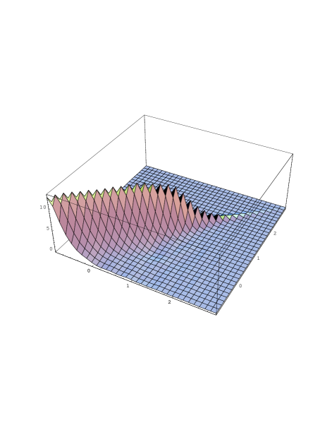
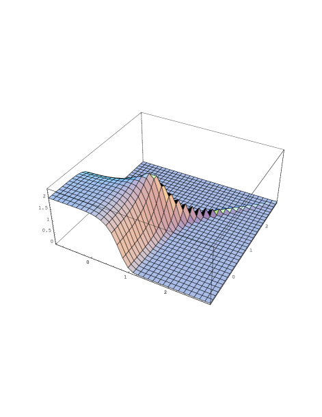
FIG. 3.: The left hand graph shows the unequal time correlation function $\langle\Theta_{00}(k,\tau_{1})\Theta^{*}_{00}(k,\tau_{2})\rangle$ from our standard scaling model. The z-axis is $\left(\tau_{1}\tau_{2}\right)^{1/2}\langle\Theta_{00}\Theta^{*}_{00}\rangle$, the x-axis is $\rm{Log}_{10}(k\tau_{1})$ and the y-axis is $\rm{Log}_{10}(k\tau_{2})$. The right hand graph shows the same plot created using the model from ref.[30].

In summary, therefore, we have outlined methods for creating source histories based on a model with two parameters, the rms speed of the strings $v$ and the persistence length $\xi$, which are measured in simulations. In doing this we have been forced to introduce various ‘system’ parameters, to allow the problem to be solved in a finite time on a discrete system, such as a computer. The value of each of these parameters was chosen, so that further increases or decreases toward the continuum value resulted in no change in the two-point functions. In particular, for results presented in this paper, we used $x_{\rm max}=1000$, $L_{i}^{1}=0.001$, $L_{i}^{2}=0.01$, $N_{S}=200$ and $F_{\rm max}=10.0$. We have also introduced the parameter $L_{f}$, quantifying the rate at which string segments are turned off. Unlike the systems parameters, $L_{f}$ clearly has some degree of physical significance. However, in section III C we demonstrate that the dependence of the results on the value of $L_{f}$ is relatively weak, and we choose to use the value $L_{f}=0.5$ for the rest of our computations.

B Power spectra for the standard scaling model

We define the standard scaling model to be one which uses the above two-point functions with the model parameters $v=0.65$ and $\xi=0.3$, measured in expanding universe simulations and an assumption of perfect scaling from defect formation to the present day. Also, we must specify a particular cosmogony and we do this by analogy to what has become called Standard Cold Dark Matter, that is, a flat background $(\Omega_{\rm tot}=1)$ spacetime comprising 95% collisionless cold dark matter and 5% baryons $(\Omega_{c}=0.95,\Omega_{b}=0.05)$, with a Hubble constant at the present day of $H_{0}=50{\rm km}\,{\rm sec}^{-1}{\rm Mpc}^{-1}$. Fig. 4 shows the resulting power spectra, normalized to COBE, for the CMB and CDM (solid lines) compared with the standard adiabatic scenario based on inflation (dot-dashed line) and the published data points with error-bars based on the assumption of Gaussianity [37, 38].

FIG. 4.: The COBE normalized angular power spectrum of CMB anisotropies, (left-hand graph) and the matter power spectrum (right-hand graph) for the standard string model (solid curve). The contributions from the defects during two time windows ($1300<z<100$ – Long dashed, $100<z<1.6$ – short dashed) are also included for comparison. Standard CDM (dot-dash curve) and observational data (data points) are included for comparison.

The CMB angular power spectrum appears to have no discernible Doppler peak for two reasons: firstly, there is a substantial ISW component to the scalar, vector and tensor anisotropies. The split into the different components is illustrated for this model in Fig. 5 and we see that the scalars are larger than the vectors, with the tensors further suppressed relative to the other two. More precisely, we find that the contributions to the angular power spectrum are in the ratio,

$$C_{l}^{S}:C_{l}^{V}:C_{l}^{T}=3:1:0.4\,,$$ (72)

at $l=10$. Although the difference between our models and those presented refs.[9, 29] are only at the level of a factor of two or so, it is still worth noting the discrepancy as a direction for future work. We suggest that this is due to a difference in super-horizon ratio of $\langle|\Theta^{S}|^{2}\rangle$ and $\langle|\Theta_{00}|^{2}\rangle$, already discussed in an earlier section.

And secondly, the component of the angular power spectrum created at the surface of last scattering is incoherent, with the secondary Doppler peaks being cancelled out by decoherence as suggested in refs.[8, 31, 32]. This leads to a further suppression of the amplitude in the ensemble average, relative to the large angular scales, since we are averaging high peaks and low troughs. We should note that although the comparison with the published CMB data does not appear to be good, the plotted error-bars are only at the level of one sigma and deviations from non-Gaussianity may require even larger errorbars, particularly for experiments with small sky coverage. We expect the situation to be much clearer when the new CMB data begins to arrive in the very near future.

FIG. 5.: The COBE normalized angular power spectrum of CMB anisotropies, (left-hand graph) and the matter power spectrum (right-hand graph) for the standard string model. The total anisotropy (solid line) is illustrated, along with the partial contributions from scalar (dotted), vector (short-dash) and tensor(long-dash) components in the case of the CMB anisotropies. The errorbars show $1\sigma$ statistical uncertainties derived from the finite number of realizations in our calculations. Observational data and the prediction for standard CDM (dot-dash curve) are also illustrated in the case of the matter power spectrum. The dotted line on the matter spectrum shows the prediction of Ref. [19], as discussed in the text.

However, the situation seems to be much more clear-cut in the case of the CDM power spectrum. Once normalized to COBE, the linear power spectrum of the CDM appears to fit the data extremely badly, with the predicted curve lying much further outside the observational errorbars than in the case of the CMB angular power spectrum. Again the errorbars are based on an assumption of Gaussianity and consideration of a non-Gaussian theory will no doubt require us to increase their size, but the level of disagreement is much larger than seems likely in any of the realistic scenarios, which are thought to be only mildly non-Gaussian on these scales. If we assume for the moment that we can compare the theoretical curves with the data in this very naive way, resolution of the absence of power on any particular scale requires us to postulate a bias between the CDM and the data. While the idea of a bias between the CDM and baryonic matter, probed by the catalogues of galaxies and clusters of galaxies which make up the dataset, is not uncommon, large values $(>2)$ are thought to be unrealistic.

The bias required on a scale of $Rh^{-1}$Mpc, where now $H_{0}=100h\,{\rm km}\,{\rm sec}^{-1}{\rm Mpc}^{-1}$, can be estimated by calculating the fractional matter over-density in a ball of radius $Rh^{-1}$Mpc,

$$\sigma^{DM}_{R}=4\pi\int{dk\over k}k^{3}P(k)|W(kR)|^{2}\,,$$ (73)

where the window function $W(x)$ is given by

$$W(x)={3\over x^{3}}\left(\sin x-x\cos x\right)\,,$$ (74)

and comparing it to $\sigma_{R}$ calculated from a hypothetical curve which fits the data, that is, $b_{R}=\sigma_{R}/\sigma_{R}^{DM}$. The scale $R=8$ corresponds to $\sigma_{R}\approx 1$, that is, scales turning non-linear at the present day, and is the most common scale on which comparisons are made. For standard CDM $\sigma_{8}=1.2$ for $h=0.5$, while the value favoured by observations is $\sigma_{8}=0.5$, illustrating the celebrated excess of power on small scales for this model. When we perform the same calculation for the string model, we get $\sigma_{8}=0.31$ and hence the bias on these scales is $b_{8}\approx 1.5$. Such a value is around the limit of what is thought to be possible, but given the uncertainties involved is not totally unreasonable.

This comparison does, however, ignore the obvious woeful absence of power on much larger scales. In order to quantify this we choose $R=100$ since (1) it is unlikely that scales of $100h^{-1}{\rm Mpc}$ are affected by non-linear gravitational evolution, (2) the distribution of galaxies is likely to be more Gaussian than on smaller scales and (3) such scales are above the neutrino free-streaming scale and so the introduction of a hot dark matter (HDM) component cannot be used to modify the shape of the spectrum. We estimate that the standard string model requires a bias of $b_{100}=5.4$ to reconcile it with the data. Since the chances of either the actual Universe[39, 40] or the physical model[41, 42] having such a bias seem remote, we conclude that the standard string model is in serious conflict with the current observations on scales around $100h^{-1}$Mpc.

The COBE normalization of our standard scaling model also allows us to calculate a value for the dimensionless quantity $G\mu$, where $\mu$ is the string mass per unit length, and $G$ is Newton’s gravitational constant. For our standard scaling model, we find that $G\mu=2.0\times 10^{-6}$, which is very close the value $G\mu=1.7\times 10^{-6}$ obtained from calculations of large angle CMB anisotropies using high resolution local string simulations[11]. Although these values are in good agreement, we stress that the purpose of our work has not been to compute $G\mu$ to high precision and we expect that variations in details of the string evolution which we have not attempted account for in our model, such as the amount of small scale structure, could give rise to variations in $G\mu$. Instead, we are primarily interested in the relative normalization of anisotropies on different scales, in particular between COBE and $\sigma_{100}$, which can be obtained without knowledge of the absolute value of $G\mu$. In future sections we present a number of variations on our standard scaling model, each giving rise to a different value for the string mass per unit length. To emphasize the fact that we do not intend to use our model to obtain precise predictions for the absolute value of $G\mu$ in realistic cosmic string scenarios, we quote all subsequent values in terms of the ratio $\mu/\mu_{S}$, where $\mu_{S}$ is the value obtained for our standard scaling model. We should note that large values of $\mu/\mu_{S}$ are likely to be excluded by the absence of residuals in timing measurements for milli-second pulsars[43].

As one final point, in Fig.5 we include the prediction for the matter power spectrum for strings in a background of CDM computed in ref.[19]. The dotted line on the matter graph shows the prediction from the I model described in this reference, normalized to give the same value for $\sigma_{8}$ as our standard scaling model. We note that the predictions are in extremely close agreement, although in the current work the amplitude is no longer arbitrary, but fixed by normalization of the associated CMB fluctuations to COBE.

C Modifications to model parameters

In order to test the robustness of the conclusions about the standard model, we have repeated the calculations for different values of $\xi$ and $v$. These variations could either represent fundamentally different types of cosmic strings to those modelled in simulations, for example, those with superconducting currents, or any possible systematic uncertainties in the measurement of these quantities. Fig. 6 shows the power spectra for different values of $\xi$ with $v=0.65$, while Fig. 7 shows the power spectra for different values of $v$ with $\xi=0.3$, with the values of $b_{100}$, $b_{8}$, and $\mu/\mu_{S}$ summarized in table I. All other parameters are as in the standard scaling model.

The first thing to note is that, although our choice of values spans the possible parameter space, none of the models does significantly better than the standard scaling case as far as the value of $b_{100}$ is concerned and there is also no discernible Doppler peak in the CMB spectrum. However, at a more microscopic level there are differences which follow the trends of previous calculations, giving us confidence that the model is reproducing intuitive results.

As $\xi$ decreases one is reducing the scale at which the two-point functions turnover from white-noise, with $\xi=2.0$ being close the causal limit [44]. It was predicted in ref.[31] that this would lead to the contribution to the CMB anisotropy from the surface of last scattering being peaked at smaller scales, which is indeed what we see in Fig. 6, although this feature is slightly masked out by the large ISW component. This can be seen more clearly in the CDM power spectrum which turns over at a scale $k\sim\xi k_{\rm eq}$. One would of course expect a reduction in $\xi$ to result in a substantially higher peak, but this is partially counter balanced by an almost equivalent increase in the ISW component, the only direct evidence for such an effect being that smaller values of $\xi$ require a smaller value of $G\mu$. This change in $G\mu$ can be understood from the formula $\rho_{s}\sim\mu/\xi^{2}$; if the value of $\xi$ decreases the value of $\mu$ must also decrease to keep the string density and hence the amplitude of the CMB anisotropy the same.

The lack of dependence on $v$ is less intuitive. One might think that in the limit of $v\rightarrow 0$, the network would become more coherent, since the strings are not moving, creating perturbations in the same place. However, such a limit does not correspond in any way to the standard picture of string evolution. If the strings are moving slowly or are stationary, then reconnection will take place only very infrequently and the scaling regime will be difficult to attain. But scaling is implicit in our model, being put in by hand, so even if they are not moving the strings will have to decay in some way, which is essentially random, introducing decoherence. The only discernible effect of changing $v$ is a weak dependence of the amplitude of the matter power spectrum, believed to be due to the dependence of the relative amplitudes of $\Theta_{00}$ and $\Theta^{S}$ on $v$ already discussed. Also interesting, however, is the apparent independence of the turnover of the matter power spectrum, suggesting that the corresponding turnover in the two-point functions is also independent of $v$. Once again the values of $b_{8}$, $b_{100}$ and $\mu/\mu_{s}$ are summarized in table I.

Description	Figure	Line type	$b_{8}$	$b_{100}$	$\mu/\mu_{S}$
Standard Scaling	4	Solid	1.61	5.36	1.0
$\xi=2.0$	6	Long-short dash	2.46	7.31	5.56
$\xi=1.0$		Dotted	2.16	6.57	2.88
$\xi=0.3$		Short-dash	1.74	5.81	1.0
$\xi=0.03$		Long-dash	1.45	5.67	0.25
$v=0.0$	7	Long-short dash	1.04	3.39	1.93
$v=0.3$		Dotted	1.27	4.13	1.64
$v=0.65$		Short-dash	1.74	5.81	1.00
$v=0.9$		Long-dash	1.66	5.58	0.92
$L_{f}=0.01$	8	Long-short dash	1.45	4.79	0.40
$L_{f}=0.1$		Dotted	1.52	5.04	0.45
$L_{f}=0.3$		Short-dash	1.64	5.45	0.56
$L_{f}=0.5$		Solid-dash	1.74	5.81	1.0
$L_{f}=0.7$		Long-dash	1.83	6.13	1.48
$L_{f}=0.9$		Dot-short dash	1.91	6.40	2.12
$h=0.3$	9	Long-short dash	2.68	6.78	0.46
$h=0.4$		Dotted	2.08	6.18	0.71
$h=0.6$		Short-dash	1.52	5.57	1.32
$h=0.7$		Long-dash	1.36	5.39	1.67
$\Omega_{b}=0.01$	10	Long-short dash	1.64	5.76	1.00
$\Omega_{b}=0.03$		Dotted	1.64	5.78	1.00
$\Omega_{b}=0.1$		Short-dash	1.87	5.86	1.00
$\Omega_{b}=0.2$		Long-dash	2.17	5.94	1.00
“Best of all worlds”	11	Long-short dash	0.3	1.56	0.03

TABLE I.: Table of biases and values of $\mu/\mu_{S}$ for the standard scaling model, and the simplest variations described in this paper. Each model is labelled by the figure and line type where it appears.

Description	Figure	Line type	$b_{8}$	$b_{100}$	$\mu/\mu_{S}$
$\tau_{T}=100$	12	Long-short dash	1.19	4.84	1.00
$\tau_{T}=400$		Dotted	0.86	3.96	1.00
$\tau_{T}=1000$		Short-dash	0.81	3.29	0.98
$\tau_{T}=5000$		Long-dash	0.93	3.09	0.84
$\chi=2$	13	Long-short dash	1.19	4.84	1.00
$\chi=5$		Dotted	0.86	3.96	1.00
$\chi=10$		Short-dash	0.81	3.29	0.98
$\chi=20$		Long-dash	0.81	3.29	0.98
$\tau_{T}=100$,$L_{T}=0.1$	14	Long-short dash	0.64	4.01	1.00
$\tau_{T}=100$,$L_{T}=0.8$		Dotted	0.37	2.59	1.00
$\tau_{T}=1000$,$L_{T}=0.1$		Short-dash	0.35	1.63	0.91
$\tau_{T}=1000$,$L_{T}=0.8$		Long-dash	0.46	1.60	0.68
$\chi=100$,varying $n$	15	Long-short dash	0.72	3.95	0.98
$\chi=400$,varying $n$		Dotted	0.38	2.37	0.97
$\chi=100$,varying $\mu$		Short-dash	0.34	1.67	0.91
$\chi=400$,varying $\mu$		Long-dash	0.54	1.81	0.57
$\alpha=0.25$	16	Long-short dash	0.56	2.66	8.16
$\alpha=0.5$		Dotted	0.20	1.33	59.96
$\alpha=0.75$		Short-dash	0.08	0.66	375.14
$\alpha=1.0$		Long-dash	0.03	0.28	1887.57
“Best of all worlds”	11	Solid dash	0.12	0.82	0.02

TABLE II.: Table of biases and values of $\mu/\mu_{S}$ for each of the models with deviations from scaling. Each model is labelled by the figure and line type where it appears.

Description	Figure	Line type	$b_{8}$	$b_{100}$	$\mu/\mu_{S}$
C1	17	Long-short dash	0.38	1.84	–
C2		Dotted	1.29	3.20	–
C3		Short-dash	6.18	19.19	–
C4		Long-dash	1.71	3.62	–
$\nu=0$	18	Long-short dash	2.10	6.14	1.23
$\nu=-1$		Dotted	2.73	9.36	0.70
$\nu=0.5$		Short-dash	1.64	4.99	1.27
$\nu=\infty$		Long-dash	2.11	7.91	–
$\epsilon=2$	19	Long-short dash	2.06	4.43	7.28
$\epsilon=5$		Dotted	1.85	4.78	2.86
$\epsilon=10$		Short-dash	1.70	4.86	1.65
$\epsilon=20$		Long-dash	1.63	5.01	1.23
$q=0$	20	Long-short dash	1.74	5.81	1.00
$q=-1$		Dotted	1.42	4.68	0.72
$q=-1.25$		Short-dash	1.52	5.04	0.77
$q=-1.5$		Long-dash	1.35	4.16	–
$q=0$	21	Long-short dash	0.54	2.55	0.07
$q=-1.0$		Dotted	0.35	1.64	0.06
$q=-1.25$		Short-dash	0.40	1.89	0.06
$q=-1.5$		Long-dash	0.19	1.00	–

TABLE III.: Table of biases and values of $\mu/\mu_{S}$ for each of the models where our standard source has been further modified. Each model is labelled by the figure and line type where it appears. Note that we have not calculated $\mu/\mu_{S}$ for coherent models, which are not based on string-like two-point functions.

FIG. 6.: Varying $\xi$, the string coherence length: We plot the COBE normalized angular power spectrum of CMB anisotropies, (left-hand graph) and the matter power spectrum (right-hand graph) for various values of the parameter $\xi$, with $v=0.65$.($\xi=2.0$ – long-short-dash line, $\xi=1.0$ – dotted line, $\xi=0.3$ – short-dash line, $\xi=0.03$ – long-dash line). Observational data and the prediction for standard CDM (dot-dash curve) are included for comparison.

FIG. 7.: Varying $v$, the string velocity: We plot the COBE normalized angular power spectrum of CMB anisotropies, (left-hand graph) and the matter power spectrum (right-hand graph) for various values of the parameter $v$, with $\xi=0.3$.($v=0.0$ – long-short-dash line, $v=0.3$ – dotted line, $v=0.65$ – short-dash line, $v=0.99$ – long-dash line). Observational data and the prediction for standard CDM (dot-dash curve) are included for comparison.

We have also tested the dependence of our results on the parameter $L_{f}$, representing the rate at which the strings are turned off. CMB and matter power spectra for various values of $L_{f}$ are illustrated in Fig. 8. The results have a weak dependence on $L_{f}$, with smaller values of $L_{f}$ giving slightly better values for $b_{100}$ than larger values. We note that further decreases in $L_{f}$ below $0.01$ do not change the results further. Since the dependence on $L_{f}$ is only weak, we choose an intermediate value of $L_{f}=0.5$ for the remaining calculations in this paper (with the exception of fig 11 in which we illustrate the possible improvement to $b_{100}$ which could result from exploiting all conceivable uncertainties in our model). The fact that the results depend minimally on $L_{f}$ also represents evidence to suggest that the results will not depend strongly on the exact way in which the decay of long string is treated.

FIG. 8.: Varying $L_{f}$, the string ‘turn off’ parameter: We plot the COBE normalized angular power spectrum of CMB anisotropies, (left-hand graph) and the matter power spectrum (right-hand graph) for various values of the parameter $L_{f}$, with $\xi=0.3$, $v=0.65$.($L_{f}=0.01$ – long-short-dash line, $L_{f}=0.1$ – dotted line, $L_{f}=0.3$ – solid line, $L_{f}=0.5$ – short-dash line, $L_{f}=0.7$ – long-dash line, $L_{f}=0.9$ – dot-short-dash line). Observational data and the prediction for standard CDM (dot-long-dash curve) are included for comparison.

D Modifications to cosmological parameters

We must also consider the possibility of different cosmogonies, since most cosmological parameters are not constrained to better than a factor two. It is simple to change the Hubble constant and also the relative content of baryons and CDM. The resulting spectra are presented in Fig. 9 for $h=0.3$ to $h=0.7$ and in Fig. 10 for $\Omega_{b}=0.01$ to $\Omega_{b}=0.2$, keeping $\Omega_{\rm tot}=1$ and using the standard scaling model for the two-point functions. Once again, no model significantly improves the value of $b_{100}$ (see table I).

The CMB angular power spectrum is largely unaffected by the changes in cosmological parameters that we have tried. However, we do see that the shape of the CDM power spectrum is modified by changes in $h$, via the time of equal-matter radiation and the well-known shape parameter $\Gamma\approx\Omega h$. This fixes the position of the turnover in the power spectrum, with larger values of $h$ leading to a turnover at smaller scales. We also notice slight oscillations in the power spectrum for larger values of $\Omega_{b}$. In these models the oscillations that are present in the photon-baryon fluid are transferred to the CDM, but in contrast to an inflationary model, they are damped out by the effects of decoherence.

FIG. 9.: Varying $h$: We plot the COBE normalized angular power spectrum of CMB anisotropies, (left-hand graph) and the matter power spectrum (right-hand graph) for various values of the cosmological expansion rate $h$, with $\Omega_{b}=0.05$. ($h=0.3$ – long-short-dash line, $h=0.4$ – dotted line, $h=0.5$ – solid line, $h=0.6$ – short-dash line, $h=0.7$ – long-dash line). Observational data and the prediction for standard CDM (dot-dash curve) are included for comparison.

FIG. 10.: Varying $\Omega_{b}$: We plot the COBE normalized angular power spectrum of CMB anisotropies, (left-hand graph) and the matter power spectrum (right-hand graph) for various values of the cosmological expansion rate $\Omega_{b}$, with $h=0.5$. ($\Omega_{b}=0.01$ – long-short-dash line, $\Omega_{b}=0.03$ – dotted line, $\Omega_{b}=0.05$ – solid line, $\Omega_{b}=0.1$ – short-dash line, $\Omega_{b}=0.2$ – long-dash line). Observational data and the prediction for standard CDM (dot-dash curve) are included for comparison.

We should comment on the apparent absence of any marked dependence on these cosmological parameters, since the CMB spectrum for $l>100$ is very strongly dependent on them in the case of the standard adiabatic scenario, and this dependence has been suggested as a way of making extremely accurate estimations of many cosmological parameters using satellite experiments. To understand this difference, we should remember that the anisotropies created at the surface of last scattering by acoustic waves are incoherent, leading an absence of secondary peaks, effectively washing out the strong dependence on $\Omega_{b}$ and $H_{0}$. And more importantly, any contribution from the last scattering surface seems to be swamped by the ISW effect, which is less sensitive to changes in the cosmogony.

One modification to the standard scenario which is often used to allow the standard cold dark matter model to obtain a better fit to the galaxy data is to introduce a small amount of hot dark matter in the form of neutrinos. A similar, procedure would also allow the standard string model to fit the shape of the observed power spectrum on scales below the neutrino free streaming scale $\lambda\approx 20h^{-1}$Mpc, but we anticipate that this will not be as efficient on larger scales, and in particular we expect the introduction of HDM to have little bearing on the $b_{100}$ problem. Nonetheless, we plan to investigate the implications of making such a changes in future work.

E Summary

In summary, we have scanned the range of each of the parameters in our model, while maintaining perfect scaling, and we have found that none of these simple variations are capable of significantly reducing the deficit of power on scales around $100h^{-1}$Mpc. However, some of the parameters do marginally improve the situation, in some cases reducing the required $b_{100}$ from $\approx 5$ to $\approx 3$. One might postulate, therefore, that modifications to all these parameters simultaneously might lead to a more substantive amount of power on 100$h^{-1}$Mpc scales, and indeed this is the case. To illustrate this, we performed a run with $\xi=0.0001$, $v=0$, $h=0.7$, $\Omega_{b}=0.01$, and $L_{f}=0.01$, which we describe as the ‘best of all worlds’ model, and the result is presented in Fig. 11. We see that the situation is improved, but still the bias required, $b_{100}=1.6$, is not unity and we now find a large excess of power on scales around $8h^{-1}$Mpc. Also, the CMB angular power spectrum appears to be worse fit to the data. While this model serves as a useful caveat to our arguments, we believe that pushing the model this far is not realistic within the current understanding of defect models. Nonetheless, it may serve as impetus for future model building.

Except for the caveat described above, the minimal dependence of $b_{100}$ on the wide variations in these parameters is already strong evidence to suggest that the $b_{100}$ problem will be a feature of most scaling defect models. In the next two sections we further test this idea by examining the results of further modifications and generalizations of the standard model, with all deviations being described as perturbations from the standard scaling model.

We should note that there are two simple variations of the cosmogony which we have ignored in the section on cosmological parameters, namely an open universe ($\Omega<1$) or the introduction of cosmological constant $(\Omega_{m}+\Omega_{\Lambda}=1)$. We anticipate that these variations will lead to modifications to scaling similar to those described in the next section [45, 46, 47, 48], and might lead to more acceptable values of $b_{100}$. An in depth investigation of this problem is the subject of ongoing research [23] (see also ref.[24]).

FIG. 11.: The “best of all worlds” models: The COBE normalized angular power spectrum of CMB anisotropies, (left-hand graph) and the matter power spectrum (right-hand graph) for the standard scaling model (dotted line) and two “best of all worlds” models. In the first of these models, (long-short dash line), the values of each of the parameters $\xi$, $v$, $h$, $\Omega_{b}$ and $L_{f}$ have been pushed as far as possible in the direction which favours high $\sigma_{100}$, while a standard scaling law is used. The second model, (solid line) is identical, except that it also incorporates a fairly plausible deviation from scaling over the matter-radiation transition. Observational data and the prediction for standard CDM (dot-dash curve) are included for comparison.

IV Variations from standard scaling

A Motivation and implementation

In the previous section, we introduced the $b_{100}$ problem for scaling defect models and showed that it is apparently robust for a range of different parameters. However, we have also noted that this scaling assumption has only been tested using defect simulations with a very small dynamic range. Hence, in the spirit of testing of the standard model, we should allow for the possibility of modifications to scaling. In fact, this is the most obvious resolution to the $b_{100}$ problem since the scaling assumption is what relates the contributions from defects on different scales. Deviating from scaling would allow us to effectively tilt the power spectrum. A similar approach has become a popular solution to the excess power on small scales in standard CDM models based inflation, but in our case we want to create more power on large scales.

This point can be illustrated most effectively by reconsidering Fig. 4 which shows the results for the standard model and also the partial contributions from the strings present in during $z=1300$ to $z=100$ (short dashed curve) and between $z=100$ and $z=1.6$ (long dashed curve). These two curves give us intuition about when the perturbations relevant for COBE normalization and $b_{100}$ are laid down. For example, if one could create an imbalance between the strings present during these two time windows, one could hope to change their relative amplitude and reconcile the current data points with COBE normalization. This is possible if one modifies the scaling picture, with most graphic illustration being the total removal of the string network around $z=100$.

The first type of deviation we consider is motivated by the mild shift in the behaviour of a string network which is observed in simulations under going a radiation-matter transition. Typically, quantities such as the string velocity, persistence length, string density, and level of small scale structure are seen to undergo a small change at around radiation-matter equality. In general, this shift tends to make strings move slower and be less dense.

One simple way to implement this step-type transition is to allow the effective energy per unit length to change, with the mass per unit length being a factor $\chi$ larger before the transition than after it. We generate histories for a source with normal scaling behaviour and then for each history, we multiply the value of each source component at each time $\tau$ by some factor $f_{R}(\tau)$. Since we require our source histories to behave smoothly, we implement a smooth shift in the value of $f_{R}$ using

$$f_{R}(\tau)=1+(\chi-1)T^{\rm off}(\tau,\tau_{T},L_{T})\,,$$ (75)

where $T^{\rm off}$ is the same smoothly varying function which was used for turning the string segments off, defined in (43), but now $L_{T}\tau_{T}$ is the starting time of the transition, and $\tau_{T}$ is the end time.

We have also tried other ways of implementing a transition, such as introducing a shift in the time dependence of the number of strings per unit volume. In the standard case, we have $n(\tau)=(\xi\tau)^{-3}$, which we modify by setting $n(\tau)=f_{R}(\tau)(\xi\tau)^{-3}$, where $f_{R}$ is the smoothly varying transition function given in (75). We find that the net results from these two ways of implementing the transition are very similar and so in the results section, we concentrate on the former, simpler case.

The second type of deviation we consider is a deviation in the scaling exponent. We implement such a transition by altering the dependence of the number of strings per unit volume on time. In the standard scaling picture, there is roughly one piece of string per correlation length cubed. Since the correlation length is proportional to the horizon size $\tau$, we find that the number density of strings as a function of time is, $n(\tau)\propto\tau^{-3}$, which we modify by setting $n(\tau)\propto\tau^{-(3+2\alpha)}$, with $\alpha=0$ being the standard value. Using (48) we see that the power spectra of the $\Theta_{\mu\nu}$’s depend on $n(\tau)$ and hence the time dependence of $\Theta_{00}$ (which behaves like the square root of the power spectrum) outside the horizon is now $\Theta_{00}=\tau^{-(\frac{1}{2}+\alpha)}$

FIG. 12.: Varying $\tau_{T}$, the end time for the modelled non-scaling radiation-matter transition: We plot the COBE normalized angular power spectrum of CMB anisotropies,(left-hand graph) and the matter power spectrum (right-hand graph) for a matter radiation transition with various values of the final time $\tau_{T}$, with $L_{T}=0.1$ and $\chi=2$.($\tau_{T}=100$ – long-short-dash line, $\tau_{T}=400$ – dotted line, $\tau_{T}=1000$ – short-dash line, $\tau_{T}=5000$ – long-dash line). Observational data and the prediction for standard CDM (dot-dash curve) are included for comparison.

FIG. 13.: Varying $\chi$, the factor by which $\mu_{\rm eff}$ is assumed to be larger before the radiation-matter transition: We plot the COBE normalized angular power spectrum of CMB anisotropies, (left-hand graph) and the matter power spectrum (right-hand graph) for a matter radiation transition with various values of the factor $\chi$, with $\tau_{T}=1000$ and $L_{T}=0.1$.($\chi=2$ – long-short-dash line, $\chi=5$ – dotted line, $\chi=10$ – short-dash line, $\chi=20$ – long-dash line). Observational data and the prediction for standard CDM (dot-dash curve) are included for comparison.

FIG. 14.: Varying $L_{T}$, the start time (in units of the end time) of the non-scaling radiation-matter transition modelled in the defect sources: We plot the COBE normalized angular power spectrum of CMB anisotropies, (left-hand graph) and the matter power spectrum (right-hand graph) for matter radiation transition models with different values of the length $L_{T}$, with amplitude $\chi=5$ ($\tau_{T}=100$, $L_{T}=0.1$ – long-short-dash line, $\tau_{T}=100$, $L_{T}=0.8$ – dotted line, $\tau_{T}=1000$, $L_{T}=0.1$ – short-dash line, $\tau_{T}=1000$, $L_{T}=0.8$ – long-dash line). Observational data and the prediction for standard CDM (dot-dash curve) are included for comparison.

FIG. 15.: Different types of non-scaling radiation-matter transitions: We plot the COBE normalized angular power spectrum of CMB anisotropies, (left-hand graph) and the matter power spectrum (right-hand graph) for two different implementations of the matter matter radiation transition, each with $\chi=5$ and $L=0.1$. ($\tau_{T}=100$, varying $n$ – long-short-dash line, $\tau_{T}=400$, varying $n$ – dotted line, $\tau_{T}=100$, varying $\mu$ – short-dash line, $\tau_{T}=400$, varying $\mu$ – long-dash line). Observational data and the prediction for standard CDM (dot-dash curve) are included for comparison.

FIG. 16.: Power law deviations from scaling: We plot the COBE normalized angular power spectrum of CMB anisotropies, (left-hand graph) and the matter power spectrum (right-hand graph) for a power law deviation from scaling with various values of the parameter $\alpha$. ($\alpha=0.25$ – long-short-dash line, $\alpha=0.5$ – dotted line, $\alpha=0.75$ – short-dash line, $\alpha=1.0$ – long-dash line). Observational data and the prediction for standard CDM (dot-dash curve) are included for comparison.

B Illustrative examples

Figs. 12, 13 and 14 illustrate the results for radiation-matter transition runs (implemented by varying $\mu$) with various choices of the parameters $\chi$, $\tau_{T}$ and $L_{T}$. The first (Fig. 12) shows mild transitions, with an amplitude $\chi=2$, each lasting for a factor of 10 in conformal time $\tau$, that is, $L_{T}=0.1$. Each curve shows results for a different choice of final time $\tau_{T}$. Initially, we see that as the time of the transition is moved later, the peak in the matter power spectrum gets higher and is shifted to larger scales. However, as discussed in the standard scaling section illustrating the two time windows, we find that as the time of the transition is increased beyond $\tau_{T}=1000$, the height of the peak in the matter power spectrum actually falls again. This is because a very late transition tends to boost the perturbations on COBE scales as well as those on scales relevant to the large scale matter power spectrum. It is clear that a transition occurring as late as today is equivalent to having no transition at all. None of these reasonable, mild transitions ($\chi=2$) significantly improves the $b_{100}$ problem.

In the second figure (Fig. 13), we stick to a transition time of $\tau_{T}=1000$, which as we have discussed gives us the best chance of introducing a shift between the COBE and large scale matter normalization. Using a transition length of $L_{T}=0.1$, we vary the amplitude $\chi$ of the transition. A value of $\chi=10$ improves things significantly on scales of $100h^{-1}$Mpc and $\chi=20$ does better still, but we find that further increases only affect the features of the matter spectrum on smaller scales. It is interesting that there is a limiting value for the relative COBE/$\sigma_{100}$ normalization, and that this limiting value happens to fit the observations very well. We note however that the cases which fit the large scale matter data require implausibly large values of the transition amplitude $\chi$, for which no precedent has been seen in studies of defect evolution. Furthermore, extremely drastic additional alterations would have to be made to the model in order to fit the small scale matter and CMB data.

In the third figure (Fig. 14), we illustrate the dependence on the length $L_{T}$ of the transition, for two different choices of the final time $\tau_{T}$, with $\chi$ fixed to be 5. We see that the length of the transition does not strongly influence the $\sigma_{100}$ normalization. In fact, we have been unable to find any region of our transition parameter space capable of fitting $\sigma_{100}$, where the choices of parameter values is more plausible than those illustrated in Fig. 13

Fig. 15 illustrates the comparison between a radiation-matter transition in which $\mu$ is varied, with one in which $n$ is varied. The first pair of curves shows a transition with $L_{T}=0.1$ and $\tau_{T}=100$. In the case where $\mu$ is varied, we choose $\chi=5$ (short-dash line) whereas in the case that $n$ is varied, we choose $\chi=25$ (long-short dash line). The reason for this difference in amplitudes is that increasing $\mu$ by a factor of $\chi$ increases the power spectrum of the perturbations by a factor of $\chi^{2}$, while the same increase in $n$ affects the power spectrum of perturbations by a factor of $\chi$. We see that the resulting spectra for this pair of models are very similar. The second pair of curves illustrate a transition with $L_{T}=0.1$ and $\tau_{T}=400$, for the same choices of $\chi$ as above. Again, the curves are very similar for each of the transition models. Hence, the resulting spectra of perturbations does not seem to be strongly dependent on the way in which the transition is implemented.

Fig. 16 shows deviations in the scaling exponent of various degrees. We see that models where the deviation from scaling is significant enough to bring about a substantial increase in the amount of power in the matter spectrum on scales around $100h^{-1}$Mpc are so extreme that they completely miss the small scale matter and CMB data. We find that further increases in the scaling exponent beyond $\alpha=1.0$ do not affect the $\sigma_{100}$ normalization, only giving rise to significant differences in the resulting power spectra on smaller scales. As in the case of the radiation-matter transition, it is interesting to note that there is a limiting value of $\sigma_{100}$ normalization with increasing alpha, and that this limiting value happens to pass through the large scale matter data.

As one final point, Fig. 11 shows the results of a relatively mild deviation from scaling (varying $\mu$, $\chi=2$, $\tau_{T}=10\tau_{eq}$, $L_{T}=0.8$) where all of the other standard parameters have been pushed as far as possible in a direction which favours a large value for $b_{100}$ as in the ‘best of all worlds model’ ($\xi=0.0001$, $v=0$, $h=0.7$, $\Omega_{b}=0.01$, and $L_{f}=0.01$) discussed earlier. In this case, $b_{100}$ is of order one. However, in obtaining a reasonable value for $b_{100}$, the resulting model totally fails to fit the shape of the matter power spectrum, with an extreme excess of power on smaller scales. Although we do not believe this limit will allow the resurrection of the standard defect scaling defect scenario, it does present a possible road of attack for the construction of more exotic models which could fit all of the data.

To summarize, we have presented results for a number of models showing deviations from scaling. None of these models is able to fit the large scale matter data without extreme corrections to the standard scaling picture, or forcing all other model parameters in the direction which favours large $b_{100}$. Even in the cases where the value of $b_{100}$ is reasonable, a very considerable amount of further work would need to be carried out in order to make the model fit small scale matter and CMB data.

V Further modifications to the model

In the previous sections we have discussed possible variations from our standard scaling string model, and we showed that only extreme deviations from the standard scaling model can significantly rectify the problem. In section III we showed how the $b_{100}$ problem is relatively robust to changes in the model parameters $v$, $\xi$ and $L_{f}$ (as well as the cosmological parameters $\Omega_{b}$ and $h$). Although all of the variations we have considered take place within the context of our string model, the robustness to these changes already provides evidence to suggest that the results will be similar for other types of defect. For instance, the independence of the results on the parameter $\xi$ suggests that results will be similar for other types of defect for which the two-point functions cut off at different sub-horizon values. In this section we further test this idea by introducing further modifications to the forms of our two-point functions by hand, in order to see how extreme these modifications must become before the $b_{100}$ situation is significantly improved.

One change which might alleviate the problem is to alter the relative strength of various components of the stress-energy. Recent work [49], which makes use of a coherent approximation to model source behaviour, has suggested that defect models with a highly suppressed anisotropic stress might give rise to more acceptable values of the matter bias factor $b$ and indeed we have already mentioned that the ratio of $\Theta^{S}$ and $\Theta_{00}$ is model dependent. In order to investigate this possibility in the context of our work, we make a simple modification to our standard scaling model. We multiply the energy $\Theta_{00}$ by $\nu$, where in models with values of $|\nu|<1$ the significance of the anisotropic stress is boosted relative to that of the energy, while in models with $|\nu|>1$, the energy is boosted. We should note that the ratio of the anisotropic stress to vector and tensor components is unaltered, as required by isotropy and causality.

Before presenting results for our full string model, we discuss the effect of these changes in the context of some simple coherent models. In Fig. 17 we present the CMB and matter power spectra for four such models. The first model (which we call C1) has

$$\Theta_{00} = \left\{\begin{array}[]{ll}\tau^{-1/2}&\quad k\tau\leq 5\,,\\ 0&\quad k\tau>5\,,\end{array}\right.$$ (78)

$$\Theta_{S} = 0\,,$$ (79)

while for the second model (C2)

$$\Theta_{00} = 0\,,$$ (80)

$$\Theta^{S} = \left\{\begin{array}[]{ll}\tau^{-1/2}&\quad k\tau\leq 5\,,\\ 0&\quad k\tau>5\,.\end{array}\right.$$ (83)

For this pair of models, the version with suppressed anisotropic stress has a more acceptable value of $b_{100}$ than the version with suppressed energy. However, this pair of models is not exactly causal, because the real space two-point correlation functions do not exactly vanish outside the horizon. We also present results for the following pair of models, which do exactly satisfy this condition. They are (C3), with

$$\Theta_{00} = \tau^{-1/2}\frac{\sin(k\tau)}{k\tau}\,,$$ (84)

$$\Theta_{S} = 0\,,$$ (85)

and (C4) with

$$\Theta_{00} = 0\,,$$ (86)

$$\Theta_{S} = \tau^{-1/2}\frac{\sin(k\tau)}{k\tau}\,.$$ (87)

The sources in the second pair of models are designed to exhibit sub-horizon decay at a similar value of $k\tau$ as the first pair of models we have discussed. However, we see that in this explicitly causal case, the model with suppressed energy actually gives a more acceptable $b_{100}$ than the model with suppressed anisotropic stress. These results represent a surprising contrast to those of the case which is not exactly causal, implying that exact imposition of causal constraints is necessary for physically meaningful results. Activity outside the causal horizon presents opportunities to seed standard ‘adiabatic’ perturbations (which will naturally make the $b_{100}$ look better). We suspect our slightly acausal model has done this to a remarkable degree.

In Fig. 18 we present the results for different values of the energy factor $\nu$, modifying our standard string two-point functions. As in the causal coherent case above, we see that $\sigma_{100}$ is actually better for models with suppressed energy rather than suppressed anisotropic stress and in fact no value of $\nu$ would give rise to a significant improvement in the $b_{100}$ problem (see table III).

FIG. 17.: Various coherent limits: We plot the COBE normalized angular power spectrum of CMB anisotropies, (left-hand graph) and the matter power spectrum (right-hand graph) for a range of coherent models discussed in the text. (Non-causal models: C1 – long-short-dash line, C2 – dotted line. Causal Models: C3 – short-dash line, C4 – long-dash line). Observational data and the prediction for standard CDM (dot-dash curve) are included for comparison.

FIG. 18.: Varying $\nu$, the enhancement factor for $\Theta_{00}$ which artificially modifies the ratio between energy and anisotropic stress: The COBE normalized angular power spectrum of CMB anisotropies, (left-hand graph) and the matter power spectrum (right-hand graph) for standard scaling subject to various values of the parameter $\nu$. ($\nu=1$ – solid line – $\nu=0$ – long-short-dash line, $\nu=-1$ – dotted line, $\nu=0.5$ – short-dash line, $\nu=\infty$ – long-dash line). Observational data and the prediction for standard CDM (dot-dash curve) are included for comparison.

Another way in which we have modified our standard model is by imposing a sharper sub-horizon cutoff in the source stress-energy. By doing this, we hope to have covered a range of possible defect behaviour including that of cosmic textures, whose stress-energy tensor will exhibit a faster sub-horizon fall-off than that of strings, reflecting the fact that they have less features on small scales. We implement this particular modification without violating the requirements of causality as follows. We introduce a parameter $\epsilon$, and specify that the number of strings with decay times $\tau_{f}$ satisfying $k\tau_{f}>\epsilon$ is zero, while the number of strings with decay times satisfying $k\tau_{f}<\epsilon$ is unchanged. Results for various choices of the parameter $\epsilon$ are shown in Fig. 19. We see that $b_{100}$ does not depend strongly on the the value of $\epsilon$.

FIG. 19.: Varying the cutoff parameter $\epsilon$: The COBE normalized angular power spectrum of CMB anisotropies, (left-hand graph) and the matter power spectrum (right-hand graph) for our standard scaling source, with various values of the parameter $\epsilon$, representing the value of $k\tau$ at which the source is subject to a sharp subhorizon cutoff. ($\epsilon=2$ – long-short-dash line, $\epsilon=5$ – dotted line, $\epsilon=10$ – short-dash line, $\epsilon=20$ – long-dash line). Observational data and the prediction for standard CDM (dot-dash curve) are included for comparison.

Finally, we allow modifications to the way in which scaling is enforced in our model. We note that our standard scaling model contains two time dependent functions, one being the number of strings per unit volume $n(\tau)$, the other $\mu(\tau)$ being the mass per unit length of the strings. In the case of standard scaling, $n(\tau)\sim\tau^{-3}$ while $\mu(\tau)$ is a constant. We note that an extreme case which would also exhibit scaling behaviour would be a model in which the number of strings $n$ was constant, but where $\mu$ evolved like $\tau^{-3/2}$. Such a case would bear some resemblance to the inflationary mimic model of Turok [33], where there is a constant number of expanding shells, but some feedback mechanism is required to modify the shell surface density in order to introduce the correct scaling behaviour. In fact, if we model $n(\tau)$ as $\tau^{-3+p}$ and $\mu(\tau)$ as $\tau^{q}$, then it is easy to verify that all models satisfying $p+2q=0$ will give rise to scaling behaviour. We modify our model by allowing variations in the parameter $q$ from the value zero. As discussed, the choice $q=-3/2$ represents a type of coherent limit. Results for such variations are shown in Fig. 20. We see that as we approach the coherent limit ($q=-3/2$) the value of $b_{100}$ is increased, but still doesn’t come close to the data.

We now present one final extreme variation on our standard scaling model, which does significantly improve the $b_{100}$ problem. Fig. 21 illustrates the effect of varying the parameter $q$ in the limit that both the string velocity and the coherence length are very small. We find that in the coherent limit ($q=-3/2$), the matter spectrum comes close to the data on large scales. So in the coherent limit, the $\sigma_{100}$ normalization depends more strongly on changes in the parameters $v$ and $\xi$ than it did in the standard, incoherent case. Although this extreme model (like the mimic model [33]) demonstrates that the $b_{100}$ problem is not a necessary consequence of the assumption of scaling, we stress that our modifications of the degree of coherence via the parameter $q$ as far as the coherent limit had no physical motivation. All known defects achieve scaling behaviour by having some kind of random decay process, such as loop production in the case of strings, or decay into Goldstone bosons during unwinding in the case of textures. Consequently, scaling seems necessarily to imply incoherence, which suggests that scaling models with constant $n(t)$ are a special, unphysical limit. We see in the figure that it is only in the coherent limit that the choice of low $\xi$ and $v$ significantly reduces the $b_{100}$ problem.

FIG. 20.: Scaling can be enforced by varying either the string density or the mass per unit length. Here we plot the COBE normalized angular power spectrum of CMB anisotropies (left-hand graph), and the matter power spectrum (right-hand graph) for a scaling source, with various values of the parameter $q$, which parameterizes the way scaling is enforced ($q=0$ corresponds to constant mass per unit length). We use $v=0.65$ and $\xi=0.3$. ($q=0$ – long-short-dash line, $q=-1$ – dotted line, $q=-1.25$ – short-dash line, $q=-1.5$ – long-dash line). Observational data and the prediction for standard CDM (dot-dash curve) are included for comparison.

FIG. 21.: Varying the scaling quality parameter $q$ with $v=0.0$ and $\xi=0.001$: We plot the COBE normalized angular power spectrum of CMB anisotropies (left-hand graph), and the matter power spectrum (right-hand graph) for a scaling source, with $q=0$ – long-short-dash line, $q=-1$ – dotted line, $q=-1.25$ – short-dash line, $q=-1.5$ – long-dash line. Observational data and the prediction for standard CDM (dot-dash curve) are included for comparison.

VI Mimic inflation and variations

One obvious counter example to the arguments we have put forward is Turok’s mimic inflation [33]. This is a scaling active model which is quite different from a standard defect model, which has been shown to produce the same structure of acoustic peaks in the small scale CMB as adiabatic theories. It is of interest here because it also manages to overcome the difficulties of the majority of models discussed in this paper by giving rise to a COBE normalized matter power with no deficit of power on large scales.

Mimic inflation is also of interest because the components of the source stress energy which are directly modelled are $\Theta_{00}+\Theta$ and $\Theta_{D}$ (as opposed to $\Theta_{00}$ and $\Theta^{S}$ which we extract in our string model). The component $\Theta_{00}+\Theta$ is particularly interesting because it accounts for essentially all of the contributions to the the scalar CMB fluctuations created at the surface of last scattering and also to the matter power spectrum.

In this section, we briefly explore variations on the mimic model in which the ratio of $\Theta_{00}+\Theta$ to $\Theta_{D}$ is allowed to vary freely. These variations do not respect the constraint $\langle\Theta_{00}\Theta^{S}\rangle\sim k^{2}$ outside the horizon. However, we believe that they are worth looking at because they illustrate a point about the relative dependence of ISW and matter contributions on $\Theta_{00}+\Theta$ and $\Theta_{D}$.

Our mimic model is based on the version presented by Hu, Spergel and White (ref. [30]). We take

$$\Theta_{00}+\Theta = C_{1}\tau^{-1/2}\frac{\sin(Ak\tau)}{(Ak\tau)}\,,$$ (88)

$$\Theta_{D} = f_{D}C_{2}\tau^{-1/2}\frac{6}{B_{2}^{2}-B_{1}^{2}}\frac{1}{k\tau}\left[\frac{\sin(B_{1}k\tau)}{(B_{1}k\tau)}-\frac{\sin(B_{2}k\tau)}{(B_{2}k\tau)}\right]\,,$$ (89)

with

$$C_{1}=(\tau\dot{a}/a)^{-1}\,,$$ (90)

and

$$C_{2}=\frac{2}{3}\frac{1}{1+4\tau\dot{a}/{a}}\,.$$ (91)

We have varied the model of [30] by multiplying $\Theta_{D}$ by a factor $f_{D}$. The results for such variations are shown in Fig. 22 (for this figure we have made use of the values $A=1$, $B_{1}=0.5$, $B_{2}=0.5$. The long-short-dash curves show the standard mimic model, normalized on COBE scales. The model has an identical acoustic peak structure to standard CDM, though the ratio of plateau to peak height is slightly higher. The matter spectrum actually lies well above the observational data. If the model is normalized to CMB data on scales larger than $l=100$, then matter spectrum lies extremely close to that of standard CDM. In other words, the mimic model matches the matter spectrum of an adiabatic model as well as the acoustic peak structure.

The short-dash curves show the results for a run where $\Theta_{D}$ is set to be 1000 times bigger than $\Theta_{00}+\Theta$. As expected, this model gives rise to extremely small contributions for the matter and oscillatory components, as compared to the ISW. The dotted curve shows the result of a run where $\Theta_{D}$ is set to zero. We see that the matter spectrum in this case is of order but slightly lower than in the basic mimic model. Therefore, the relative amplitude of matter and ISW contributions seems to depend in a non trivial way on the relative amplitude of $\Theta_{D}$ and $\Theta_{00}+\Theta$, except in the limit that $\Theta_{00}+\Theta$ is small.

In Fig. 23 we show the results of varying the $f_{D}$ for different choices of the parameters $A$, $B_{1}$ and $B_{2}$, which we vary by multiplying each one by a factor $f_{p}$ from its original value. We see that with $f_{p}=0.4$, the matter power spectrum lacks power on large scales in the standard case of $f_{D}=1.0$. However, this deficit of power can be made up for by setting $f_{D}=0.0$. The resulting matter power spectrum is in strikingly good agreement with the observational data. This is in contrast to the case $f_{P}=1.0$ where the effect of reducing $f_{D}$ to zero is to diminish the matter spectrum.

To summarize, the results of this section illustrate that models can be constructed which are capable of solving the $b_{100}$ problem. However the examples of this and previous sections have also indicated that changes in the parameters can give contradictory results, particularly in the coherent limit. We re-emphasize that in the coherent limit there is no physical motivation for the concept of scaling (which comes about as a result of random processes in all known scaling models). Furthermore, the case which gave a good fit to the matter spectrum did not satisfy constraints on the superhorizon anisotropic stress that are required by isotropy. Nevertheless, these are interesting cases which should be investigated further to see if they could give rise to plausible models of structure formation.

FIG. 22.: Variations on the Mimic inflation model: We plot the COBE normalized angular power spectrum of CMB anisotropies (left-hand graph), and the matter power spectrum (right-hand graph) for variations on the mimic inflation model. The amplitude of the $\Theta_{D}$ component is multiplied by a factor $f_{D}$, with $f_{D}=1.0$ (long-short-dash line), $f_{D}=0.0$ (dotted line) and $f_{D}=1000$ (long-dash line). Observational data and the prediction for standard CDM (dot-dash curve) are included for comparison.

FIG. 23.: Further variations on the Mimic inflation model: We plot the COBE normalized angular power spectrum of CMB anisotropies (left-hand graph), and the matter power spectrum (right-hand graph) for variations on the parameters $A$, $B_{1}$, $B_{2}$. The amplitude of these parameters is varied from the standard case by multiplying each one by a factor $f_{p}$. Also the ratio of $\Theta_{00}+\Theta$ to $\Theta_{D}$ is varied by multiplying $\Theta_{D}$ by a factor $f_{D}$. We take $f_{p}=1.0$, $f_{D}=1.0$ (dot-dash line), $f_{p}=0.4$, $f_{D}=1.0$ (dot line), $f_{p}=1.0$ $f_{D}=0.0$ (short-dash line), $f_{p}=0.4$ $f_{D}=0.0$ (short-dash line). Observational data and the prediction for standard CDM (dot-dash curve) are included for comparison.

VII Discussion and conclusions

Substantial progress has been made in understanding the predictions from cosmic defect models of structure formation. The modern state-of-the-art calculations[9, 10, 11] all represent significant advances over previous work[19, 52, 53, 54, 12, 55, 13, 56, 15, 50]. While our ‘Modeling’ approach is not as explicitly tied to simulations as the work of Pen et al [9] and Allen et al [11], its strength is that it allows us to probe the robustness of our key results, as a function of variations in the defect stress-energy histories. This lets us investigate possible variations among different defect models and possible systematic uncertainties in the simulations.

We have found a serious conflict between standard scaling defect models and the current observational data. This conflict can be clearly expressed in terms of the ‘$b_{100}$ problem’, where $b_{100}$ is the bias on scales of $100h^{-1}$Mpc. Current theoretical and experimental results indicate that the actual value of $b_{100}$ is close to unity, but the standard defect models we considered, once COBE normalized, required $b_{100}\approx 5$ to reconcile the predictions for the density field fluctuations with the observed galaxy distribution. The problem is robust over a wide variations in parameters describing the defect sources and over variations in $\Omega_{b}$ and $h$ as well. It is tempting to exploit current uncertainties in the standard scaling picture to resurrect the defect picture, but we have found that truly radical deviations from the standard scaling assumption are required to produce a more viable model. While one variation from the standard model could get $b_{100}\approx 1.6$ (or even of order 1 if a deviation from scaling is introduced as well), to get this close is done at the expense of totally failing to fit the shape of the matter spectrum and most of our ideas about how defects interact and evolve would also have to be wrong.

Structure formation on $100h^{-1}$Mpc scales is not strongly affected by changes in the matter content, and we do not expect that changes in the dark matter could save the scaling defect models. Probably the most interesting direction to take the standard defect scenario is toward an open universe or one with a non vanishing cosmological constant. There have been some suggestions [46] that sufficient deviations from scaling might be realized in some low $\Omega_{0}$ or cosmological constant models to result in a viable scenario. We also discovered a handful of very different scaling models (see table III) which had more reasonable values of $b_{100}$, but which have very little to do with the standard defect scenarios. They may however, represent interesting directions for future model building.

Our results were anticipated in a number of ways by earlier work. Pen, Spergel and Turok (ref.[12]) noted a serious bias problem for specific global defect models on scales up to $20h^{-1}$ Mpc and the compilation of refs.[19] and [15] in ref.[57] looks very much like our results (and the shape of the CDM curve in ref.[19] is almost identical to ours). However, in each case it was far from clear that sufficient dynamic range had been achieved to predict the COBE normalized density field accurately. One of the strengths of our current method is that dynamic range is not a problem and we feel we have covered the range of other possible uncertainties in the ‘model scanning’ described in sections III-V. In cases where comparisons are appropriate, our results are consistent with those of Pen, Seljak and Turok [9], where dynamic range is also not a problem.

Our results are extremely negative for the standard scaling defect models and it is essential that results of this significance are critically scrutinized. We see four possible areas where this scrutiny might be directed.

• Linear Einstein-Boltzmann solver : We have used standard technology to solve the linearized Einstein-Boltzmann equations. Initially, we modified a passive scalar code to include sources and we checked this with the equivalent code used in ref.[9]. The vector and tensor codes have not at this stage been checked. We should note, however, that an accurate Einstein-Boltzmann solver is the ultimate quantitative authority in this subject and that analytic fitting formulae have only limited usage if they do not agree. Calculations based on these fitting formulae may be wrong by up to a factor of two.

• Modeling of two-point functions : Clearly, our results depend on our choices of defect stress-energy two-point functions, which were designed to fit flat space string simulations. We have extensively probed variations about these two-point functions and we found that only much less motivated models are even marginally consistent with the data. Nonetheless, we have illustrated that some models, which at this stage are physically unmotivated, can fit the data on 100$h^{-1}$Mpc. Obviously, much more work will be done on this subject.

• Bias : It appears that $b_{100}\approx 5$ (or even $b_{100}\approx 3$) is not consistent with the data and also that defect models are unable to generate such a large bias. If either of these turns out to be false the case against defects will be weakened.

• Comparison with data : It is essential that we have made the comparison with the data correctly. If the current data turns out to be dramatically inaccurate, our conclusions would of course change. A more subtle problem might be the assumption of Gaussianity which goes into producing the error bars used in the comparisons between theory and data. We believe that the dependence of the error bars on the sample size, be it the sky coverage in a CMB experiment or the depth of a redshift survey, is likely to be very model dependent. Although the central limit theorem seems to ensure that the comparisons we make are reasonable in most defect models[58, 59], in more exotic cases[60] the effect can be large.

We have carefully scrutinized all four of these issues, and, at this stage, stand by our conclusions. However, we are happy to engage in critical dialogues on these topics.

Much of the early calculations of defect models have involved various heuristic arguments, particularly concentrating on the effect of an individual defect on the microwave background or on matter accretion. Such approaches were able to give an intuitive picture of the effects of defects on structure formation, but in the modern age we feel strongly that arguments such as ‘model X does not look so bad’ must be translated into expressions for the two-point functions before we are willing to take them seriously — factors of two can be important and would obviously change the conclusions of this work. We have also demonstrated that results from coherent models can have very little to do with the fully active decoherent case and that it is essential that causality be strictly enforced if physically meaningful results are to be obtained. We are not arguing against the utility of heuristic discussions, but it is essential for the heuristic pictures to be brought into contact with the modern calculations if they are to have an impact.

The complete failure of the bulk of the models we considered here is in striking contrast with the (inflation motivated) nearly scale invariant adiabatic models (which have no trouble getting $b_{100}$ right). These two types of model are different in many ways and it is not necessarily easy to pin the problems on a single physical difference. Still, it is worth noting a number of effects which all cause problems for the defect scenarios.

Firstly, the defect models are isocurvature models and passive isocurvature models are know to have the CDM perturbation at a given wavelength (relative to temperature perturbations at the same wavelength) down by a factor of $6$ as compared with the adiabatic case. A similar effect is present in the active cases[61], although this is not directly relevant to the $b_{100}$ problem, which compares temperature and CDM fluctuations on different scales. The scaling (or other) assumption which links these two scales is a crucial part of the story. This difference between defect and adiabatic models is more directly connected with the problem of matching the galaxy data with the smaller scale CMB measurements, for example, within the early time window of Fig. 4, a matter which is problematic for defects, but which we have not emphasized here.

Secondly, the growth of the CDM perturbations under gravitational collapse is crucial to both pictures. The fact that defect models lay down perturbations throughout time (as compared with the inflationary models, for which the perturbations are ‘set up’ early on) means that the average defect perturbation benefits less from the gravitational collapse. The temperature perturbations benefit more equally from the constant active seeding, so this is another physical effect which suppresses the relative perturbations in matter versus radiation.

Finally, the previous effect is further enhanced by the generic presence of vector and tensor perturbations in the active models. These do not excite growing modes in the CDM, but make added contributions to the temperature fluctuations, especially on COBE scales.

Having made these points, we must emphasize that the ability for a causal active model to duplicate the successes of an adiabatic model are purely a technical matter. There is no formal ‘no go theorem’ against active models, it is just that the models which best match our current ideas about defects don’t work. The best counter example is Turok’s ‘inflationary mimic’ model[33]. We have confirmed Turok’s conjecture that the mimic model produces adiabatic-like predictions for the CDM spectrum, as well as for the CMB anisotropies (which were the original focus in [33]), and we have added a few new scaling models to the list. We are also investigating a number of physical processes which could produce extremely non-scaling sources. All these models are, however, radical departures from the original standard scaling defect picture and they require further work to determine if they correspond to realistic physical scenarios.

The problems with the standard defect models are likely to have a significant impact on our understanding of the origin of cosmic structure. The defect models were the classic examples of models of structure formation in which Standard Big Bang (SBB) causality holds. That is, one started with a perfectly homogeneous universe and seeded perturbations via causal processes in the SBB. With the demise of the standard defect models, the question arises whether any plausible SBB causal model exists. If the answer is negative, then this is very strong evidence for an inflationary origin of cosmic structure, in which SBB causality is violated to produce fluctuations of the standard ‘adiabatic’ form. We are currently investigating the other possibilities of SBB causal models of structure formation mentioned above, but it is too early to tell if a convincing scenario can emerge.

REFERENCES

- [1] V.M.H. Ruutu et al, Nature 382, 334 (1996).
- [2] T.W.B. Kibble, J. Phys. A9, 1387 (1976).
- [3] A. Vilenkin & E.P.S. Shellard, Cosmic strings and other topological defects (Cambridge University Press, 1994).
- [4] M. Hindmarsh & T.W.B. Kibble, Rep. Prog. Phys. 58, 477 (1995).
- [5] Ya.B. Zel’dovich, MNRAS 192, 663 (1980).
- [6] A. Vilenkin [1981], Phys. Rev. Lett. 46, 1169. Erratum: Phys. Rev. Lett. 46, 1496.
- [7] N. Turok, Phys. Rev. Lett. 63, 2625 (1989).
- [8] A. Albrecht, D. Coulson, P.G. Ferreira and J. Magueijo, Phys. Rev. Lett. 76, 1413 (1996).
- [9] U.L. Pen, U. Seljak and N.Turok, Phys. Rev. Lett. 79, 1615 (1997).
- [10] A. Albrecht, R.A. Battye and J. Robinson, astro-ph/9707129, Phys. Rev. Lett. in press.
- [11] B. Allen, R.R. Caldwell, S. Dodelson, L. Knox, E.P.S. Shellard and A. Stebbins, Phys. Rev. Lett. 79, 2624 (1997).
- [12] U.L. Pen, D.N. Spergel and N.Turok, Phys. Rev. D49, 692 (1994).
- [13] R.G. Crittenden & N. Turok, Phys. Rev. Lett. 75, 2642 (1995).
- [14] R. Durrer, A. Gangui & M. Sakellariadou, Phys. Rev. Lett. 76, 579 (1996).
- [15] B. Allen, R.R. Caldwell, E.P.S. Shellard, A. Stebbins and S. Veeraraghavan, Phys. Rev. Lett. 77, 3061 (1996).
- [16] T.W.B. Kibble [1985], Nucl. Phys. B252, 227. Erratum: Nucl. Phys. B261, 750.
- [17] D. Austin, E.J. Copeland and T.W.B. Kibble, Phys. Rev. D48, 5594 (1993).
- [18] C.J.A.P. Martins and E.P.S. Shellard, Phys. Rev. D54, 2535 (1996).
- [19] A. Albrecht and A. Stebbins, Phys. Rev. Lett. 68, 2121; ibid 69 2615 (1992).
- [20] A. Albrecht and N. Turok, Phys. Rev. D40, 973 (1989).
- [21] D. Bennett and F. Bouchet, Phys. Rev. D41, 2408 (1990).
- [22] B. Allen and E.P.S. Shellard, Phys. Rev. Lett. 64, 119 (1990).
- [23] R.A. Battye, J. Robinson and A. Albrecht, astro-ph/9711336.
- [24] P.P. Avelino, E.P.S. Shellard, J.H. Wu and B. Allen, In prep.
- [25] U. Seljak, Ap. J. 435, L87 (1994). W. Hu and N. Sugiyama, Ap. J. 444, 489 (1995).
- [26] P.J.E. Pebbles and J.T. Yu, Ap. J. 162, 815 (1970). M.L. Wilson and J.Silk, Ap. J. 243, 14 (1981). P.J.E. Peebles, Ap. J. 248, 885 (1981). J.R Bond and A. Salzay, Ap. J. 274, 443 (1983). N. Vittorio and J. Silk, Ap. J. 285, L39 (1984). J.R. Bond and G. Efstathiou, Ap. J. 285, L45 (1984). J. Bernstein and S. Dodelson, Phys. Rev. D41, 354 (1990). S. Dodelson and J.M. Jubas, Ap. J. 439, 503 (1995). C.-P. Ma and E. Bertschinger, Ap. J. 455, 7 (1995).
- [27] W. Hu and M. White, astro-ph/9702170.
- [28] U. Seljak and M. Zaldarriaga, Ap. J. 469, 437 (1996).
- [29] N. Turok, U.L. Pen and U. Seljak, astro-ph/9706250.
- [30] W.Hu, M. White and D. Spergel, Phys. Rev. 55, 3288 (1997).
- [31] J. Magueijo, A. Albrecht, D. Coulson and P.G. Ferreira, Phys. Rev. Lett. 76, 2617 (1996).
- [32] J. Magueijo, A. Albrecht, D. Coulson and P.G. Ferreira, Phys. Rev. D54, 3727 (1996).
- [33] N. Turok, Phys. Rev. D54, R3686 (1996).
- [34] N. Turok, Phys. Rev. Lett. 77, 4138 (1996).
- [35] G.R. Vincent, M. Hindmarsh and M. Sakellariadou, Phys. Rev. D55, 573 (1997).
- [36] A. Albrecht, R.A. Battye and J. Robinson, In prep.
- [37] The data points have been compiled by M. Tegmark at http://www.sns.ias.edu/ max/cmb/experiments.html
- [38] J.A. Peacock and S.J. Dodds, MNRAS 267, 1020 (1994).
- [39] E. Gaztanaga and J. Frieman, Ap. J. L13, 137 (1994).
- [40] J.A. Willick, M.A. Strauss, A. Dekel and T. Kolatt, astro-ph/9612240.
- [41] T. Abel et al, astro-ph/9706262.
- [42] B. Wandelt, In preparation.
- [43] R.R. Caldwell, R.A. Battye and E.P.S. Shellard, Phys. Rev. D54, 7146 (1997).
- [44] J. Robinson and B. Wandelt, Phys. Rev. D53, 618 (1996).
- [45] C.J.A.P. Martins, Phys. Rev. D55, 5208 (1997).
- [46] C. van de Bruck, astro-ph/9705208.
- [47] P. Ferreira, Phys. Rev. Lett. 74, 3522 (1995).
- [48] P.P. Avelino, R.R. Caldwell and C.J.A.P. Martins, Phys. Rev. D56, 4568 (1997).
- [49] R. Durrer and M. Sakellariadou, astro-ph/9702028.
- [50] R. Durrer, M. Kunz, C. Lineweaver and M. Sakellariadou, astro-ph/9706215.
- [51] R. Durrer and M.Kunz, astro-ph/9711133.
- [52] D. Bennett, A. Stebbins and F. Bouchet, Ap. J. 399, L5 (1992).
- [53] D. Bennett and S. Rhie, Ap. J. 406, L7 (1993).
- [54] R. Moessner, L. Perivolaropoulos and R. Brandenberger, Ap. J. 425, 365 (1994).
- [55] D. Coulson, P. Ferreira, P. Graham and N. Turok, Nature 368, 27 (1994).
- [56] R. Durrer and Z.H. Zhou, Phys. Rev. D53, 5394 (1996).
- [57] M. White and D. Scott, Comm. on Astro. 18, 289 (1996).
- [58] N. Turok, Ap. J. 473, L5 (1996).
- [59] J. Robinson and A. Albrecht, M.N.R.A.S 283, 733 (1996).
- [60] C. Cheung and J. Magueijo, astro-ph/9707271.
- [61] A. Jaffe, A. Stebbins and J. Frieman, Ap. J. 420, 9 (1994).